Lab 2 Practice
Donghyung Lee
2019-09-05
Last updated: 2019-09-13
Checks: 7 0
Knit directory: STA_463_563_Fall2019/
This reproducible R Markdown analysis was created with workflowr (version 1.4.0). The Checks tab describes the reproducibility checks that were applied when the results were created. The Past versions tab lists the development history.
Great! Since the R Markdown file has been committed to the Git repository, you know the exact version of the code that produced these results.
Great job! The global environment was empty. Objects defined in the global environment can affect the analysis in your R Markdown file in unknown ways. For reproduciblity it’s best to always run the code in an empty environment.
The command set.seed(20190905) was run prior to running the code in the R Markdown file. Setting a seed ensures that any results that rely on randomness, e.g. subsampling or permutations, are reproducible.
Great job! Recording the operating system, R version, and package versions is critical for reproducibility.
Nice! There were no cached chunks for this analysis, so you can be confident that you successfully produced the results during this run.
Great job! Using relative paths to the files within your workflowr project makes it easier to run your code on other machines.
Great! You are using Git for version control. Tracking code development and connecting the code version to the results is critical for reproducibility. The version displayed above was the version of the Git repository at the time these results were generated.
Note that you need to be careful to ensure that all relevant files for the analysis have been committed to Git prior to generating the results (you can use wflow_publish or wflow_git_commit). workflowr only checks the R Markdown file, but you know if there are other scripts or data files that it depends on. Below is the status of the Git repository when the results were generated:
Ignored files:
    Ignored:    .DS_Store
    Ignored:    .Rproj.user/

Unstaged changes:
    Modified:   README.md
Note that any generated files, e.g. HTML, png, CSS, etc., are not included in this status report because it is ok for generated content to have uncommitted changes.
These are the previous versions of the R Markdown and HTML files. If you’ve configured a remote Git repository (see ?wflow_git_remote), click on the hyperlinks in the table below to view them.
| File | Version | Author | Date | Message |
|---|---|---|---|---|
| Rmd | 95b04a6 | dleelab | 2019-09-13 | added |
| Rmd | 5f075a3 | dleelab | 2019-09-13 | repo updated |
| html | 69adea1 | statslee | 2019-09-06 | html built |
| Rmd | 5c642d9 | statslee | 2019-09-06 | created |
An Intro to R data programming
Base R tools:
* classes
* numeric summaries
* basic plots
New R tools:
* tidyverse (is a collection of R packages)
* ggplot2 package: advanced graphics
* dplyr package: data manipulation, working with data frames
Part 1: Object Type
icecream <- read.table("data/icecream.txt")
dim(icecream)
[1] 200 5copier <- read.table("data/CH01PR20.txt")
dim(copier)[1] 45 2Understand Dataframe
class(icecream)[1] "data.frame"class(copier)[1] "data.frame"head(icecream) id female ice_cream video puzzle
1 70 0 2 47 57
2 121 1 1 63 61
3 86 0 3 58 31
4 141 0 3 53 56
5 172 0 1 53 61
6 113 0 1 63 61head(copier) V1 V2
1 20 2
2 60 4
3 46 3
4 41 2
5 12 1
6 137 10colnames(copier)=c("minutes","number")
head(copier) minutes number
1 20 2
2 60 4
3 46 3
4 41 2
5 12 1
6 137 10#alternative way
copier <- setNames(copier,c("minutes","number"))
head(copier) minutes number
1 20 2
2 60 4
3 46 3
4 41 2
5 12 1
6 137 10dim(icecream)[1] 200 5names(icecream)[1] "id" "female" "ice_cream" "video" "puzzle" class(icecream$video)[1] "integer"head(iris) Sepal.Length Sepal.Width Petal.Length Petal.Width Species
1 5.1 3.5 1.4 0.2 setosa
2 4.9 3.0 1.4 0.2 setosa
3 4.7 3.2 1.3 0.2 setosa
4 4.6 3.1 1.5 0.2 setosa
5 5.0 3.6 1.4 0.2 setosa
6 5.4 3.9 1.7 0.4 setosaclass(iris$Species)[1] "factor"class(iris$Sepal.Length)[1] "numeric"Class type can be changed
class(icecream$video)[1] "integer"x=as.numeric(icecream$video)
class(x)[1] "numeric"Check the difference of the following to different types
x [1] 47 63 58 53 53 63 53 39 58 50 53 63 61 55 31 50 50 58 55 53 66 72 55
[24] 61 39 39 61 58 39 55 47 64 66 72 61 61 66 66 36 39 42 58 55 50 63 69
[47] 49 63 53 47 57 47 50 55 69 26 33 56 58 44 58 69 34 36 36 50 55 42 65
[70] 44 39 58 63 74 58 45 49 63 39 42 55 61 66 63 44 63 53 42 34 61 47 66
[93] 69 44 47 63 66 69 39 61 69 66 33 50 61 42 50 51 50 58 61 39 46 59 55
[116] 42 55 58 58 39 50 50 39 48 34 58 44 50 47 29 50 54 50 47 44 67 58 44
[139] 42 44 44 50 39 44 53 48 55 44 40 34 42 58 50 53 58 55 54 47 42 61 53
[162] 51 63 61 55 40 61 47 55 53 50 47 31 61 35 54 55 53 58 56 50 39 63 50
[185] 66 58 53 42 55 53 42 50 55 34 50 42 36 55 58 53y=as.factor(x)
class(y)[1] "factor"y [1] 47 63 58 53 53 63 53 39 58 50 53 63 61 55 31 50 50 58 55 53 66 72 55
[24] 61 39 39 61 58 39 55 47 64 66 72 61 61 66 66 36 39 42 58 55 50 63 69
[47] 49 63 53 47 57 47 50 55 69 26 33 56 58 44 58 69 34 36 36 50 55 42 65
[70] 44 39 58 63 74 58 45 49 63 39 42 55 61 66 63 44 63 53 42 34 61 47 66
[93] 69 44 47 63 66 69 39 61 69 66 33 50 61 42 50 51 50 58 61 39 46 59 55
[116] 42 55 58 58 39 50 50 39 48 34 58 44 50 47 29 50 54 50 47 44 67 58 44
[139] 42 44 44 50 39 44 53 48 55 44 40 34 42 58 50 53 58 55 54 47 42 61 53
[162] 51 63 61 55 40 61 47 55 53 50 47 31 61 35 54 55 53 58 56 50 39 63 50
[185] 66 58 53 42 55 53 42 50 55 34 50 42 36 55 58 53
34 Levels: 26 29 31 33 34 35 36 39 40 42 44 45 46 47 48 49 50 51 53 ... 74z=as.character(x)
class(z)[1] "character"z [1] "47" "63" "58" "53" "53" "63" "53" "39" "58" "50" "53" "63" "61" "55"
[15] "31" "50" "50" "58" "55" "53" "66" "72" "55" "61" "39" "39" "61" "58"
[29] "39" "55" "47" "64" "66" "72" "61" "61" "66" "66" "36" "39" "42" "58"
[43] "55" "50" "63" "69" "49" "63" "53" "47" "57" "47" "50" "55" "69" "26"
[57] "33" "56" "58" "44" "58" "69" "34" "36" "36" "50" "55" "42" "65" "44"
[71] "39" "58" "63" "74" "58" "45" "49" "63" "39" "42" "55" "61" "66" "63"
[85] "44" "63" "53" "42" "34" "61" "47" "66" "69" "44" "47" "63" "66" "69"
[99] "39" "61" "69" "66" "33" "50" "61" "42" "50" "51" "50" "58" "61" "39"
[113] "46" "59" "55" "42" "55" "58" "58" "39" "50" "50" "39" "48" "34" "58"
[127] "44" "50" "47" "29" "50" "54" "50" "47" "44" "67" "58" "44" "42" "44"
[141] "44" "50" "39" "44" "53" "48" "55" "44" "40" "34" "42" "58" "50" "53"
[155] "58" "55" "54" "47" "42" "61" "53" "51" "63" "61" "55" "40" "61" "47"
[169] "55" "53" "50" "47" "31" "61" "35" "54" "55" "53" "58" "56" "50" "39"
[183] "63" "50" "66" "58" "53" "42" "55" "53" "42" "50" "55" "34" "50" "42"
[197] "36" "55" "58" "53"Change the variable ice_cream to factor
icecream$ice_cream [1] 2 1 3 3 1 1 1 1 1 1 1 1 3 3 2 2 3 1 3 1 1 1 1 3 1 1 3 1 3 2 1 3 3 1 3
[36] 3 1 3 2 1 1 1 1 2 3 2 3 1 1 1 1 3 1 1 1 3 2 1 1 1 1 3 2 1 3 1 1 2 2 1
[71] 1 3 1 1 1 2 3 3 1 3 3 2 1 2 1 3 3 3 1 3 1 2 3 2 2 2 1 3 2 3 3 3 2 3 1
[106] 1 3 2 2 3 1 2 3 2 3 1 3 3 2 2 2 1 1 1 2 3 1 1 3 2 1 2 1 1 2 3 1 1 1 1
[141] 2 3 1 1 1 3 1 1 2 2 2 3 1 1 1 1 1 1 1 3 2 1 3 2 1 2 1 2 1 2 2 1 3 3 2
[176] 2 1 1 3 2 1 1 3 1 3 2 1 1 3 2 2 3 1 3 1 1 1 1 1 3class(icecream$ice_cream)[1] "integer"icecream$ice_cream=as.factor(icecream$ice_cream)
icecream$ice_cream [1] 2 1 3 3 1 1 1 1 1 1 1 1 3 3 2 2 3 1 3 1 1 1 1 3 1 1 3 1 3 2 1 3 3 1 3
[36] 3 1 3 2 1 1 1 1 2 3 2 3 1 1 1 1 3 1 1 1 3 2 1 1 1 1 3 2 1 3 1 1 2 2 1
[71] 1 3 1 1 1 2 3 3 1 3 3 2 1 2 1 3 3 3 1 3 1 2 3 2 2 2 1 3 2 3 3 3 2 3 1
[106] 1 3 2 2 3 1 2 3 2 3 1 3 3 2 2 2 1 1 1 2 3 1 1 3 2 1 2 1 1 2 3 1 1 1 1
[141] 2 3 1 1 1 3 1 1 2 2 2 3 1 1 1 1 1 1 1 3 2 1 3 2 1 2 1 2 1 2 2 1 3 3 2
[176] 2 1 1 3 2 1 1 3 1 3 2 1 1 3 2 2 3 1 3 1 1 1 1 1 3
Levels: 1 2 3class(icecream$ice_cream)[1] "factor"Part 2: Exploratory Data Analysis
(1) Numerical summaries:
-mean, median, five number summary, standard deviation, IQR, correlation, etc.
Traditional R
mean(icecream$video)[1] 51.85median(icecream$video)[1] 53sd(icecream$video)[1] 9.900891var(icecream$video)[1] 98.02764summary(icecream$video) Min. 1st Qu. Median Mean 3rd Qu. Max.
26.00 44.00 53.00 51.85 58.00 74.00 IQR(icecream$video)[1] 14cor(copier$minutes,copier$number)[1] 0.978517summary(icecream) id female ice_cream video
Min. : 1.00 Min. :0.000 1:95 Min. :26.00
1st Qu.: 50.75 1st Qu.:0.000 2:47 1st Qu.:44.00
Median :100.50 Median :1.000 3:58 Median :53.00
Mean :100.50 Mean :0.545 Mean :51.85
3rd Qu.:150.25 3rd Qu.:1.000 3rd Qu.:58.00
Max. :200.00 Max. :1.000 Max. :74.00
puzzle
Min. :26.00
1st Qu.:46.00
Median :52.00
Mean :52.41
3rd Qu.:61.00
Max. :71.00 summary(copier) minutes number
Min. : 3.00 Min. : 1.000
1st Qu.: 36.00 1st Qu.: 2.000
Median : 74.00 Median : 5.000
Mean : 76.27 Mean : 5.111
3rd Qu.:111.00 3rd Qu.: 7.000
Max. :156.00 Max. :10.000 Advanced summary statistics (tidyverse)
“tibbles” instead of R’s traditional data.frame. Tibbles are data frames, but they tweak some older behaviours to make life a little easier.
Install and load R package “dplyr”
#install.packages("dplyr")
library(dplyr)
Attaching package: 'dplyr'The following objects are masked from 'package:stats':
filter, lagThe following objects are masked from 'package:base':
intersect, setdiff, setequal, unionAverage and standard deviation by icecream flavor
Use %>%(pipe). You can read it as a series of imperative statements: group, then summarise, then filter. A good way to pronounce %>% when reading code is “then”.
icecream %>% group_by(ice_cream) %>%
  summarise(Mean=mean(puzzle),Variance=var(puzzle))
# A tibble: 3 x 3
ice_cream Mean Variance
<fct> <dbl> <dbl>
1 1 52.0 99.5
2 2 47.3 117.
3 3 57.1 99.2puzzle.summary <-icecream %>% group_by(ice_cream) %>%
summarise(Mean=mean(puzzle), Variance=var(puzzle) )
puzzle.summary# A tibble: 3 x 3
ice_cream Mean Variance
<fct> <dbl> <dbl>
1 1 52.0 99.5
2 2 47.3 117.
3 3 57.1 99.2class(puzzle.summary)[1] "tbl_df" "tbl" "data.frame"puzzle.summary <- icecream %>% group_by(ice_cream) %>%
summarise(Mean=mean(puzzle),
Variance=var(puzzle) )%>%as.data.frame()
puzzle.summary ice_cream Mean Variance
1 1 52.03158 99.45644
2 2 47.31915 117.43941
3 3 57.13793 99.24380class(puzzle.summary)[1] "data.frame"Behind the scenes, x %>% f(y) turns into f(x, y), and x %>% f(y) %>% g(z) turns into g(f(x, y), z) and so on. You can use the pipe to rewrite multiple operations in a way that you can read left-to-right, top-to-bottom.
dplyr verbs
‘filter’,‘arrange’,‘mutate’,‘summarise’,‘group_by’
filter: select cases based on their values
head(icecream) id female ice_cream video puzzle
1 70 0 2 47 57
2 121 1 1 63 61
3 86 0 3 58 31
4 141 0 3 53 56
5 172 0 1 53 61
6 113 0 1 63 61icecream <- as_tibble(icecream)
icecream# A tibble: 200 x 5
id female ice_cream video puzzle
<int> <int> <fct> <int> <int>
1 70 0 2 47 57
2 121 1 1 63 61
3 86 0 3 58 31
4 141 0 3 53 56
5 172 0 1 53 61
6 113 0 1 63 61
7 50 0 1 53 61
8 11 0 1 39 36
9 84 0 1 58 51
10 48 0 1 50 51
# … with 190 more rowsicecream %>% filter(female==0)# A tibble: 91 x 5
id female ice_cream video puzzle
<int> <int> <fct> <int> <int>
1 70 0 2 47 57
2 86 0 3 58 31
3 141 0 3 53 56
4 172 0 1 53 61
5 113 0 1 63 61
6 50 0 1 53 61
7 11 0 1 39 36
8 84 0 1 58 51
9 48 0 1 50 51
10 75 0 1 53 61
# … with 81 more rowsicecream %>% filter(female==1, video<50)# A tibble: 41 x 5
id female ice_cream video puzzle
<int> <int> <fct> <int> <int>
1 8 1 2 44 48
2 129 1 2 47 51
3 1 1 2 39 41
4 47 1 2 33 41
5 65 1 1 42 56
6 4 1 2 39 51
7 131 1 3 46 66
8 106 1 1 42 41
9 37 1 2 39 51
10 73 1 1 39 56
# … with 31 more rowsiris %>% filter(Species=="setosa", Sepal.Width>4) Sepal.Length Sepal.Width Petal.Length Petal.Width Species
1 5.7 4.4 1.5 0.4 setosa
2 5.2 4.1 1.5 0.1 setosa
3 5.5 4.2 1.4 0.2 setosairis %>% filter(Species=="versicolor", Petal.Length<4) Sepal.Length Sepal.Width Petal.Length Petal.Width Species
1 4.9 2.4 3.3 1.0 versicolor
2 5.2 2.7 3.9 1.4 versicolor
3 5.0 2.0 3.5 1.0 versicolor
4 5.6 2.9 3.6 1.3 versicolor
5 5.6 2.5 3.9 1.1 versicolor
6 5.7 2.6 3.5 1.0 versicolor
7 5.5 2.4 3.8 1.1 versicolor
8 5.5 2.4 3.7 1.0 versicolor
9 5.8 2.7 3.9 1.2 versicolor
10 5.0 2.3 3.3 1.0 versicolor
11 5.1 2.5 3.0 1.1 versicolor# Question: filter iris dataset for Species equal to "setosa" or "virginica"arrange: reorder cases
icecream %>% arrange(video) # order 'video' column in ascending order# A tibble: 200 x 5
id female ice_cream video puzzle
<int> <int> <fct> <int> <int>
1 15 0 3 26 42
2 45 1 2 29 26
3 38 0 2 31 56
4 51 1 3 31 39
5 67 0 2 33 32
6 47 1 2 33 41
7 134 0 2 34 46
8 133 0 1 34 31
9 44 1 2 34 46
10 46 1 2 34 41
# … with 190 more rowsicecream %>% arrange(desc(puzzle)) # order 'puzzle' column in descending order# A tibble: 200 x 5
id female ice_cream video puzzle
<int> <int> <fct> <int> <int>
1 95 0 3 61 71
2 192 0 3 66 71
3 183 0 1 55 71
4 100 1 3 69 71
5 180 1 3 58 71
6 139 1 1 55 71
7 59 1 1 55 71
8 23 1 2 58 71
9 143 0 1 72 66
10 154 0 3 61 66
# … with 190 more rowsas_tibble(iris) %>% arrange(Petal.Length)# A tibble: 150 x 5
Sepal.Length Sepal.Width Petal.Length Petal.Width Species
<dbl> <dbl> <dbl> <dbl> <fct>
1 4.6 3.6 1 0.2 setosa
2 4.3 3 1.1 0.1 setosa
3 5.8 4 1.2 0.2 setosa
4 5 3.2 1.2 0.2 setosa
5 4.7 3.2 1.3 0.2 setosa
6 5.4 3.9 1.3 0.4 setosa
7 5.5 3.5 1.3 0.2 setosa
8 4.4 3 1.3 0.2 setosa
9 5 3.5 1.3 0.3 setosa
10 4.5 2.3 1.3 0.3 setosa
# … with 140 more rowsas_tibble(iris) %>% arrange(desc(Sepal.Length))# A tibble: 150 x 5
Sepal.Length Sepal.Width Petal.Length Petal.Width Species
<dbl> <dbl> <dbl> <dbl> <fct>
1 7.9 3.8 6.4 2 virginica
2 7.7 3.8 6.7 2.2 virginica
3 7.7 2.6 6.9 2.3 virginica
4 7.7 2.8 6.7 2 virginica
5 7.7 3 6.1 2.3 virginica
6 7.6 3 6.6 2.1 virginica
7 7.4 2.8 6.1 1.9 virginica
8 7.3 2.9 6.3 1.8 virginica
9 7.2 3.6 6.1 2.5 virginica
10 7.2 3.2 6 1.8 virginica
# … with 140 more rows# Question: 1) filter iris dataset for Species equal to "setosa" and 2) sort in descending order of Sepal.Width mutate: add new variables that are functions of existing variables
icecream_new <- icecream %>% mutate(puzzle100 = puzzle*100)
icecream_new
# A tibble: 200 x 6
id female ice_cream video puzzle puzzle100
<int> <int> <fct> <int> <int> <dbl>
1 70 0 2 47 57 5700
2 121 1 1 63 61 6100
3 86 0 3 58 31 3100
4 141 0 3 53 56 5600
5 172 0 1 53 61 6100
6 113 0 1 63 61 6100
7 50 0 1 53 61 6100
8 11 0 1 39 36 3600
9 84 0 1 58 51 5100
10 48 0 1 50 51 5100
# … with 190 more rows# Question: 1) filter icecream dataset for ice_cream equal to 1, 2) create video1000 (video*1000) column, 3) sort in descending order of video1000, 4) assign the dataset to icecream_new2summarise: condense multiple values to a single value
icecream %>% summarise(Mean_video=mean(video), SD_video=sd(video), SD_median=median(video))# A tibble: 1 x 3
Mean_video SD_video SD_median
<dbl> <dbl> <dbl>
1 51.8 9.90 53group_by: break down a dataset into specified groups of rows
puzzle.summary <- icecream %>% group_by(ice_cream) %>% summarise(Mean=mean(puzzle),
            Variance=var(puzzle))%>%as.data.frame()

iris %>% group_by(Species) %>% summarise(Mean=mean(Sepal.Length), Median=median(Sepal.Length), Variance=var(Sepal.Length))
# A tibble: 3 x 4
Species Mean Median Variance
<fct> <dbl> <dbl> <dbl>
1 setosa 5.01 5 0.124
2 versicolor 5.94 5.9 0.266
3 virginica 6.59 6.5 0.404# Question: 1) group by Species 2) calculate mean, median, var, min, max for each group 3) sort data in descending order of mean 3) convert to a data frame 4) assign the output to "iris_new"Graphical plots:
- 1 variable: boxplots, histograms, etc.
- 2 variables: scatterplot
- more variables: scatterplot matrix
Traditional R plotting
Density plot, boxplot
plot(density(copier$minutes),xlab="minutes")#,ylab="density")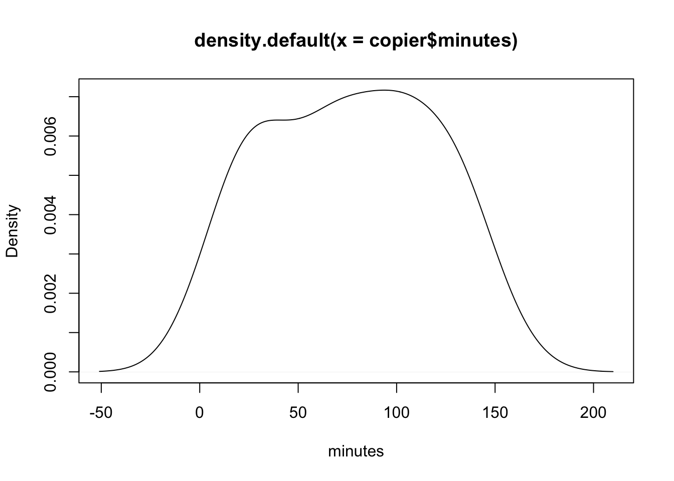
| Version | Author | Date |
|---|---|---|
| 69adea1 | statslee | 2019-09-06 |
plot(density(icecream$puzzle),xlab="puzzle score")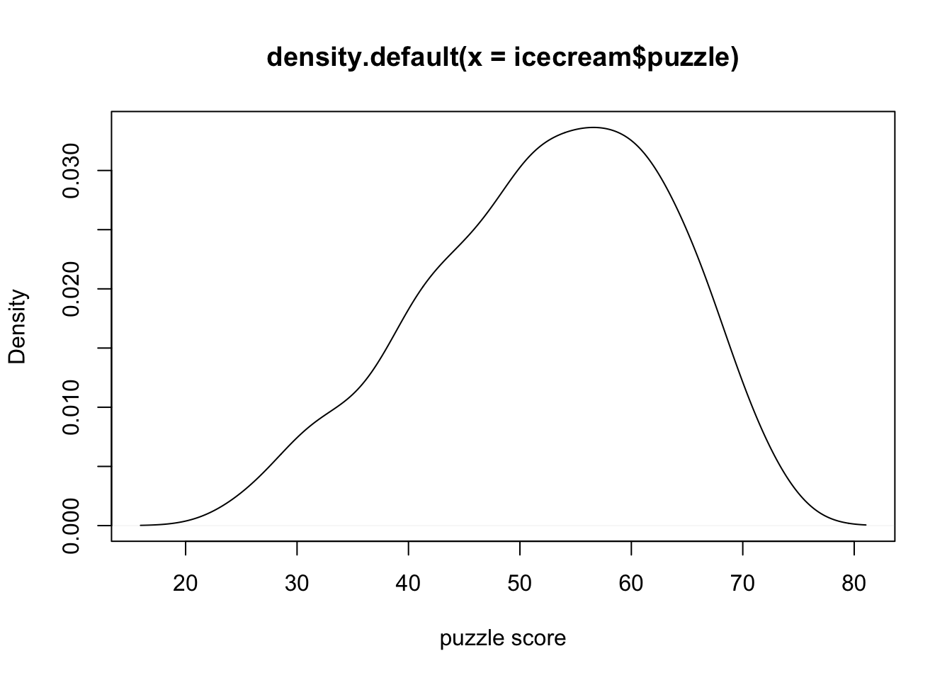
| Version | Author | Date |
|---|---|---|
| 69adea1 | statslee | 2019-09-06 |
boxplot(video~ice_cream, data=icecream)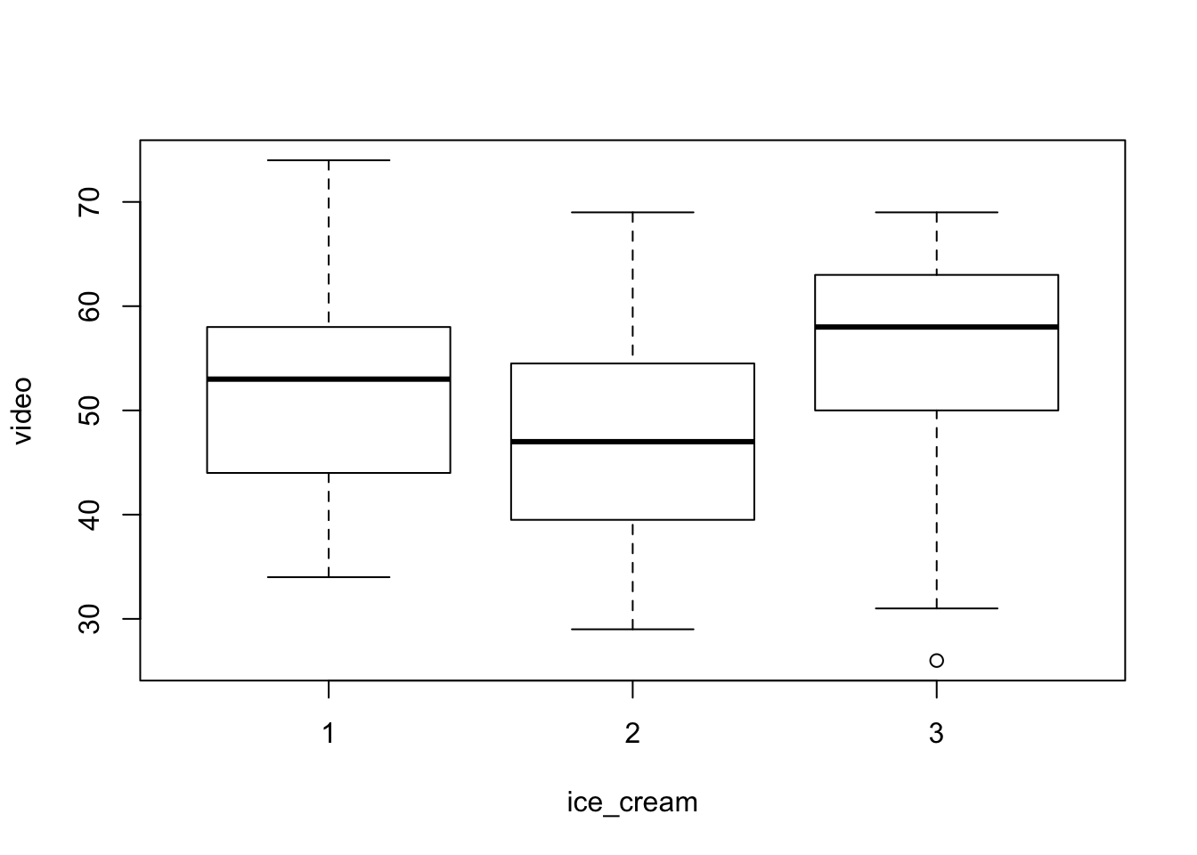
| Version | Author | Date |
|---|---|---|
| 69adea1 | statslee | 2019-09-06 |
Scatter plot
plot(x=copier$number,y=copier$minutes)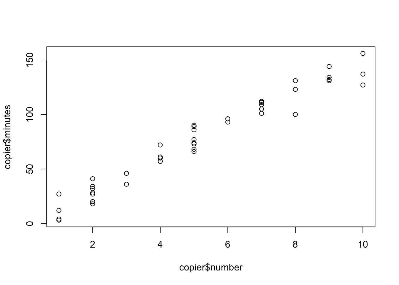
| Version | Author | Date |
|---|---|---|
| 69adea1 | statslee | 2019-09-06 |
plot(puzzle~video, data=icecream)#response againt predictors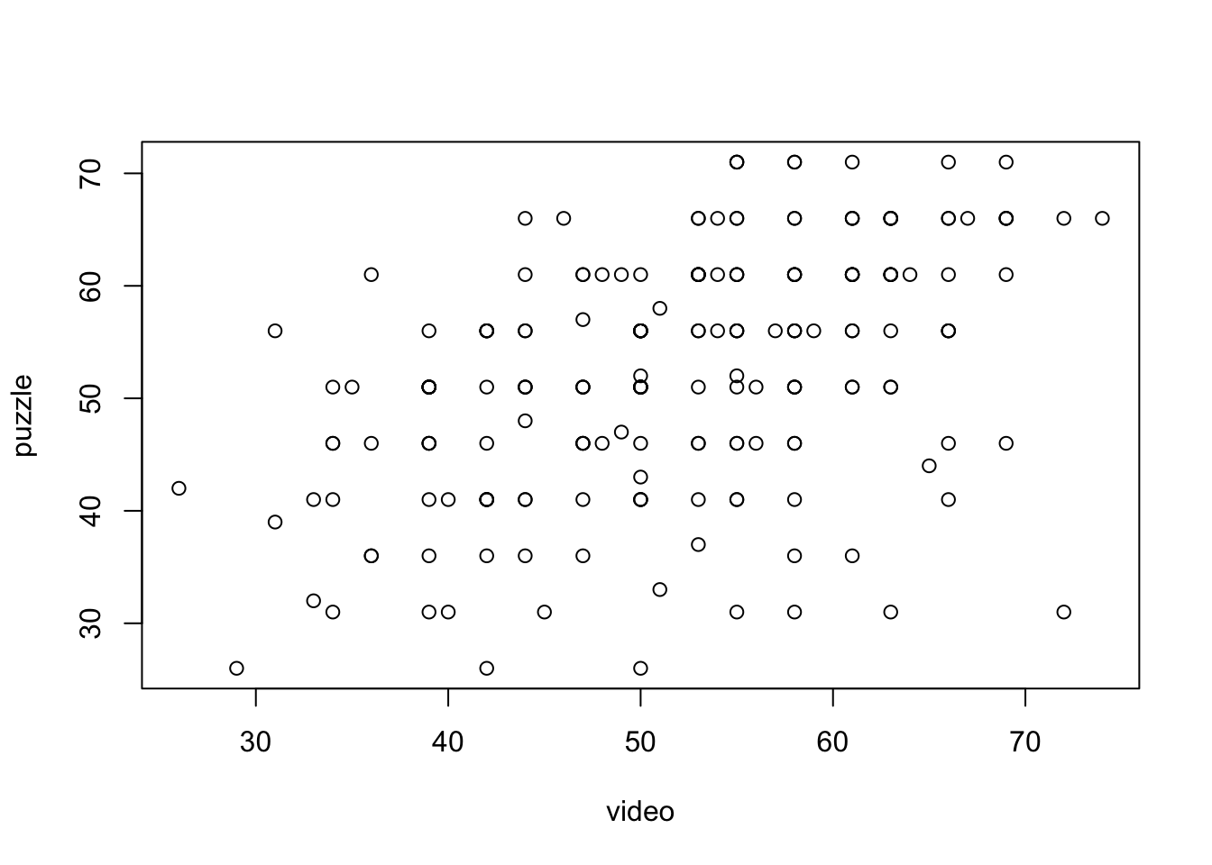
| Version | Author | Date |
|---|---|---|
| 69adea1 | statslee | 2019-09-06 |
# by default, it's x axis first, then y axis. or you can specifyCorrelation matrix
head(iris) Sepal.Length Sepal.Width Petal.Length Petal.Width Species
1 5.1 3.5 1.4 0.2 setosa
2 4.9 3.0 1.4 0.2 setosa
3 4.7 3.2 1.3 0.2 setosa
4 4.6 3.1 1.5 0.2 setosa
5 5.0 3.6 1.4 0.2 setosa
6 5.4 3.9 1.7 0.4 setosacor(iris[,1:3]) Sepal.Length Sepal.Width Petal.Length
Sepal.Length 1.0000000 -0.1175698 0.8717538
Sepal.Width -0.1175698 1.0000000 -0.4284401
Petal.Length 0.8717538 -0.4284401 1.0000000pairs(iris[,1:3])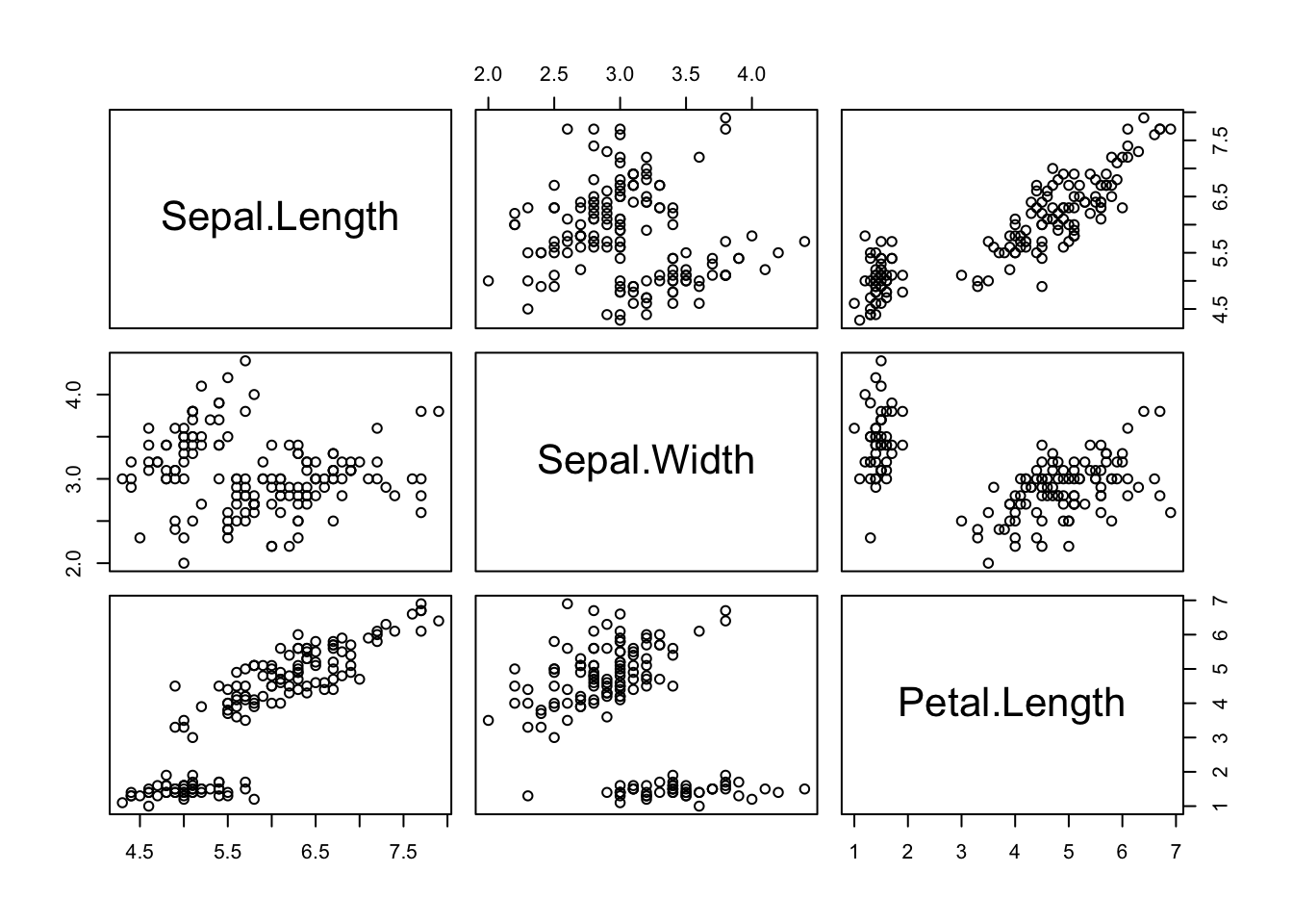
| Version | Author | Date |
|---|---|---|
| 69adea1 | statslee | 2019-09-06 |
Advanced ploting - ggplot2
#install.packages("ggplot2")
library(ggplot2)
Density plot
Run the first layer, then add extra layers, use + to add extra layers
p <- ggplot(data=copier, mapping=aes(x=minutes)) +
  geom_density() +
  xlab("Minutes used") +
  ggtitle("This is a density plot of minutes") +
  theme(plot.title = element_text(hjust = 0.5))
p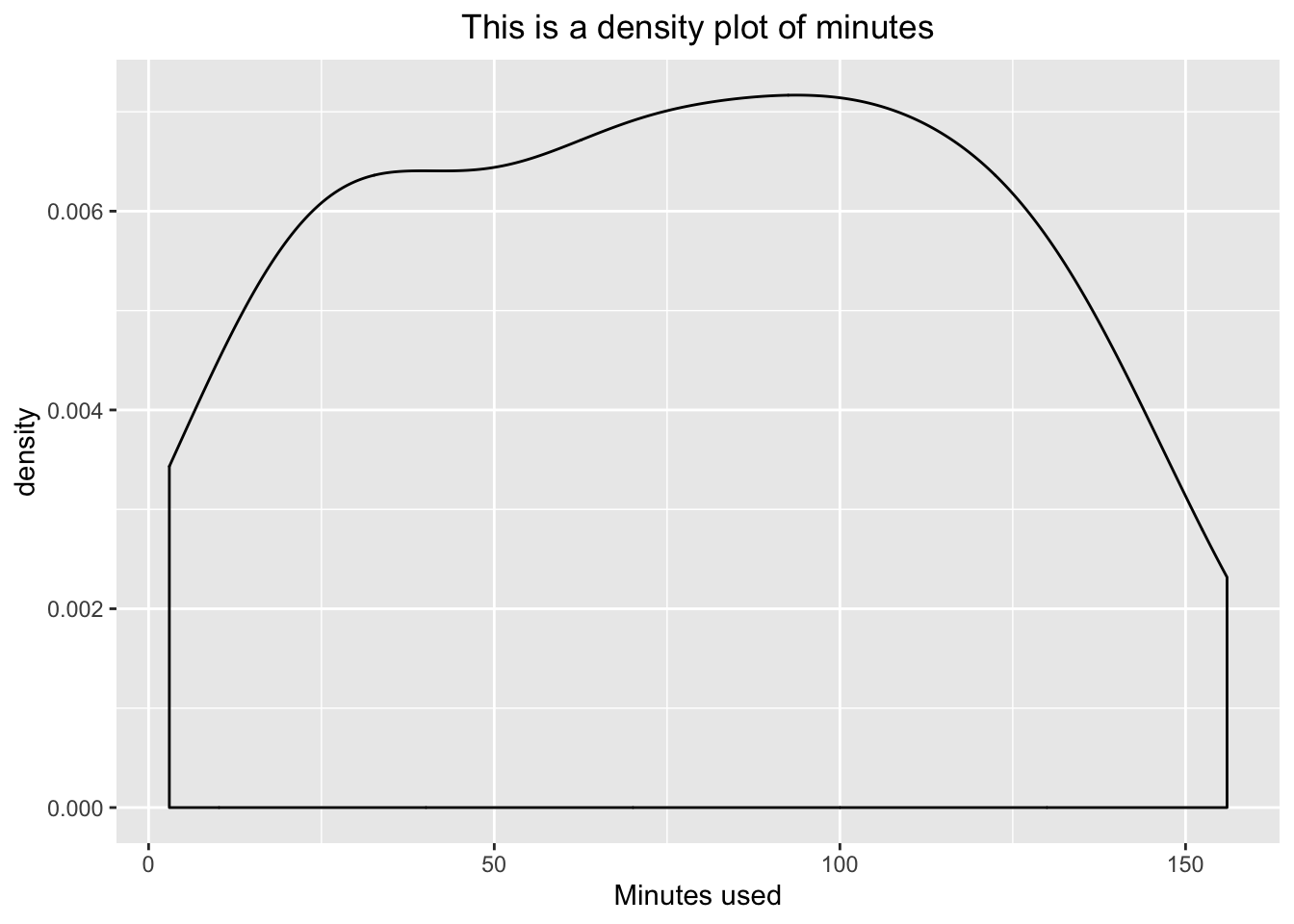
| Version | Author | Date |
|---|---|---|
| 69adea1 | statslee | 2019-09-06 |
Add mean line(vertical line)
p + geom_vline(aes(xintercept=mean(minutes)),
color="red", linetype="dashed", size=2) #change dotted, or size 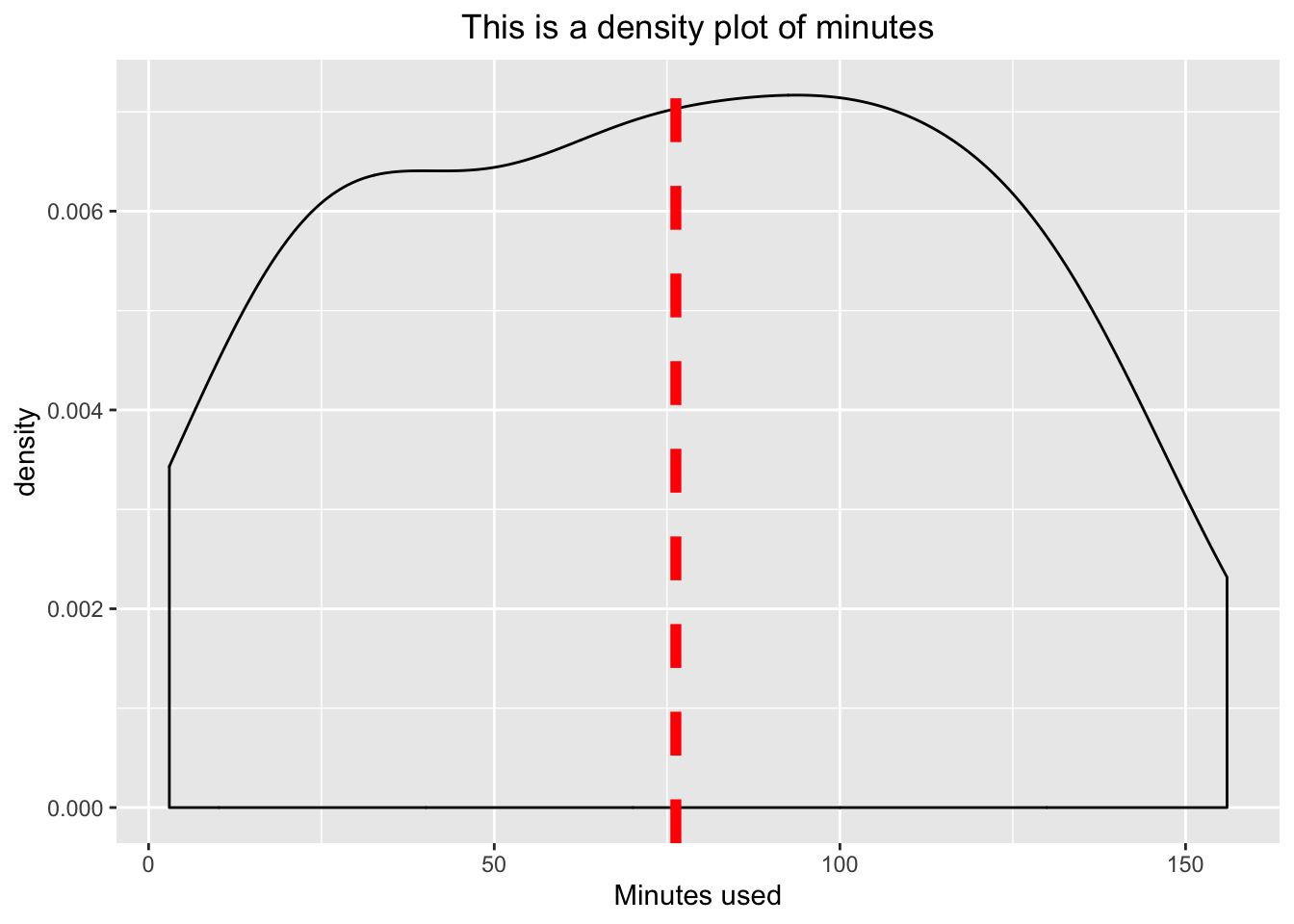
| Version | Author | Date |
|---|---|---|
| 69adea1 | statslee | 2019-09-06 |
A geom is the geometrical object that a plot uses to represent data. People often describe plots by the type of geom that the plot uses. For example, bar charts use bar geoms, line charts use line geoms, boxplots use boxplot geoms, and so on. Scatterplots break the trend; they use the point geom. As we see above, you can use different geoms to plot the same data.
Boxplot
p <- ggplot(icecream, aes(x=ice_cream, y=puzzle)) +
  geom_boxplot()
p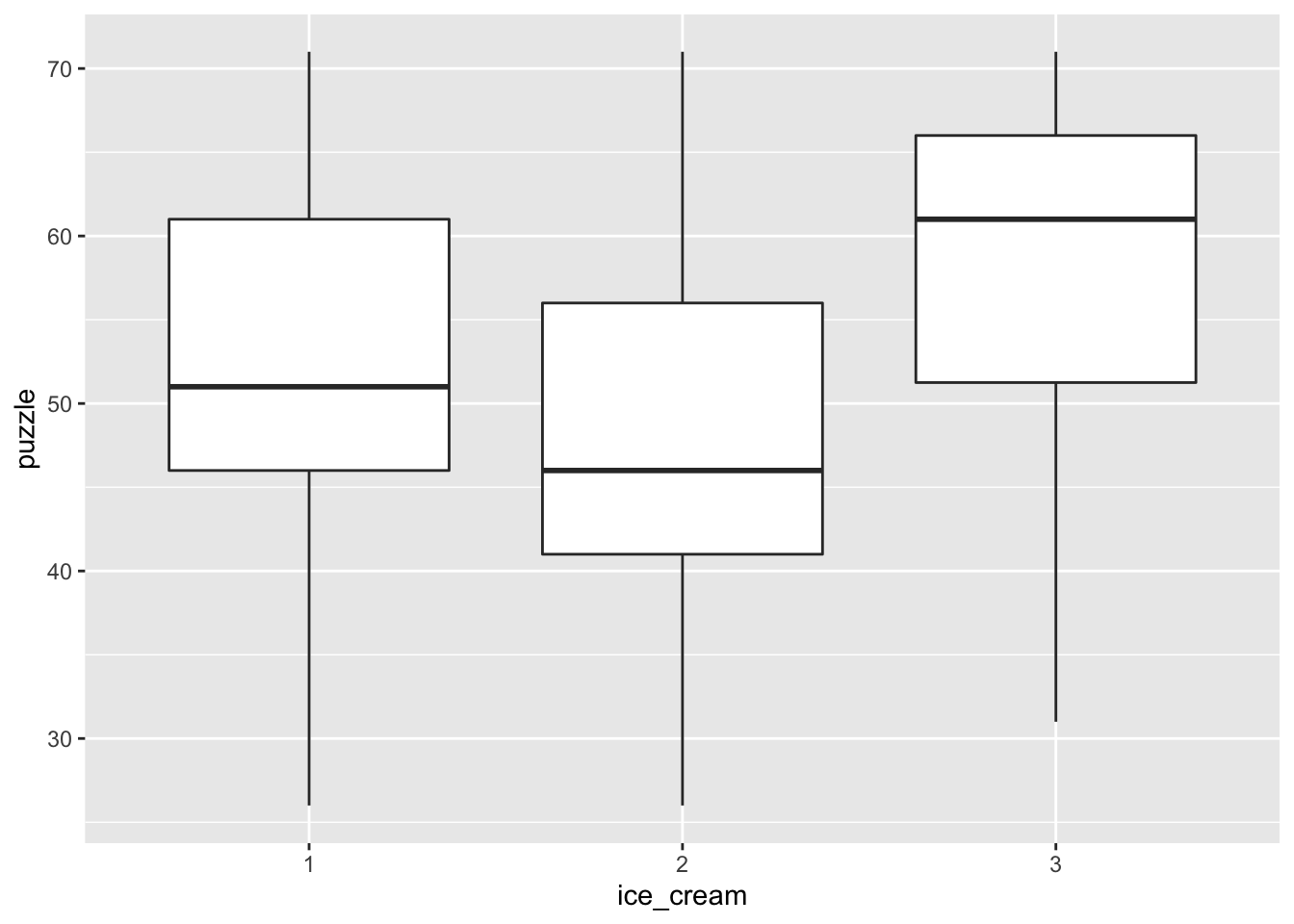
| Version | Author | Date |
|---|---|---|
| 69adea1 | statslee | 2019-09-06 |
Similar method
q <- ggplot(icecream) +
  geom_boxplot(aes(x=ice_cream, y=puzzle) )
q
| Version | Author | Date |
|---|---|---|
| 69adea1 | statslee | 2019-09-06 |
Add summary stats
q + geom_point(data=puzzle.summary,aes(x=ice_cream, y=Mean), shape=18, col="blue", size=3)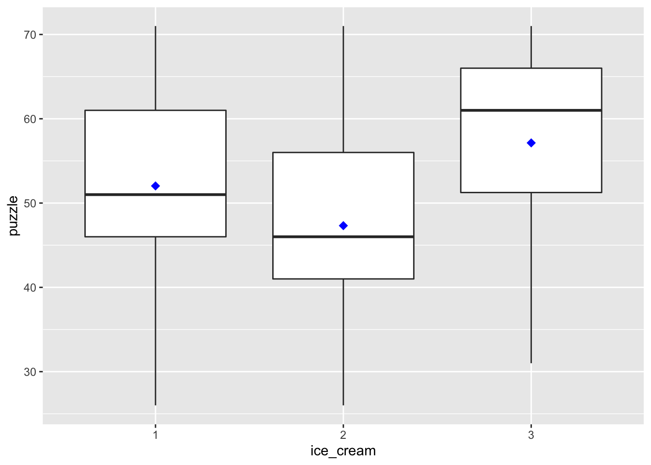
| Version | Author | Date |
|---|---|---|
| 69adea1 | statslee | 2019-09-06 |
p + stat_summary(fun.y=mean, geom="point", shape=7,col="red", size=4)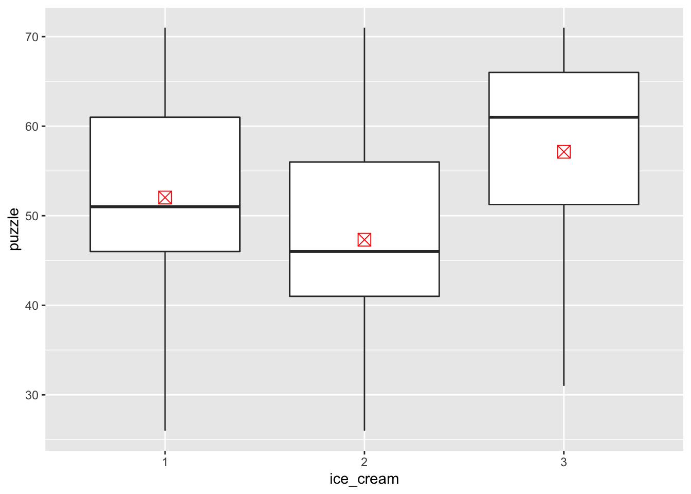
| Version | Author | Date |
|---|---|---|
| 69adea1 | statslee | 2019-09-06 |
q + stat_summary(aes(x=ice_cream, y=puzzle),fun.y=mean, geom="point", shape=7,col="red", size=4)
| Version | Author | Date |
|---|---|---|
| 69adea1 | statslee | 2019-09-06 |
#a little bit different, q don't have the aes settings, just different ways to do the calculation. Scatter plot - copier data
p <- ggplot(copier,aes(x=number, y=minutes)) +
  geom_point()
p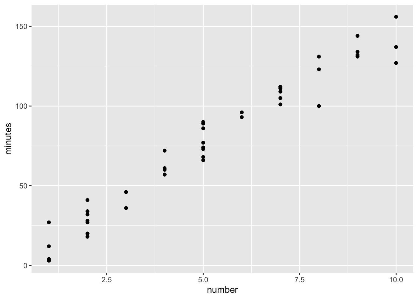
| Version | Author | Date |
|---|---|---|
| 69adea1 | statslee | 2019-09-06 |
Change theme
p + theme_bw()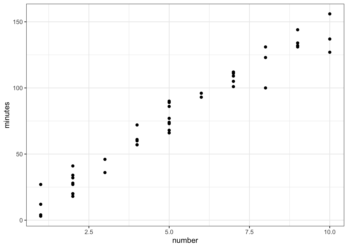
| Version | Author | Date |
|---|---|---|
| 69adea1 | statslee | 2019-09-06 |
p + theme_classic()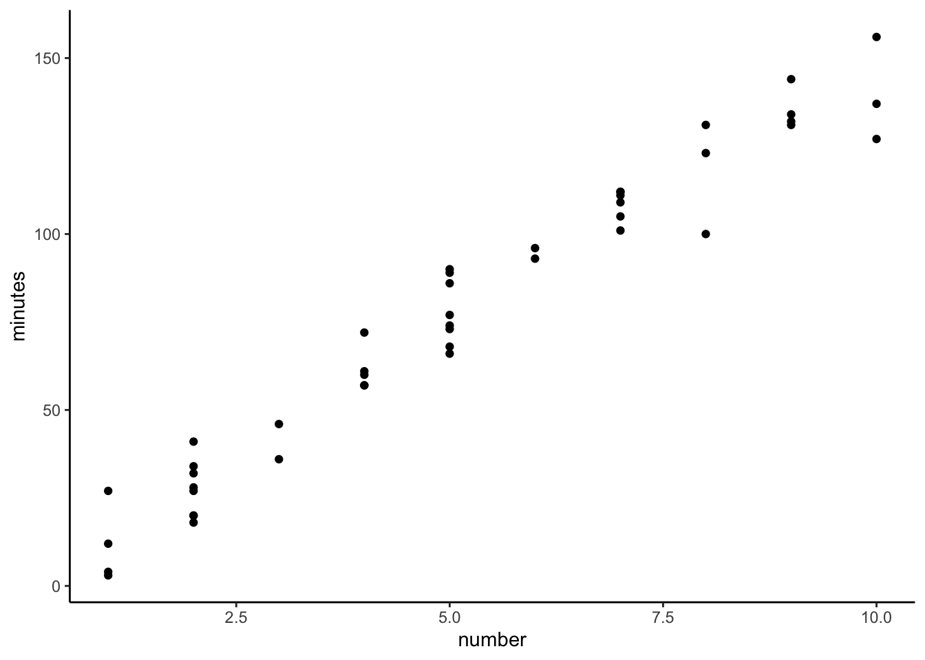
| Version | Author | Date |
|---|---|---|
| 69adea1 | statslee | 2019-09-06 |
Scatter plot - icecream data
p <- ggplot(icecream,aes(x=video, y=puzzle, col=ice_cream,shape=ice_cream)) +
  geom_point()
p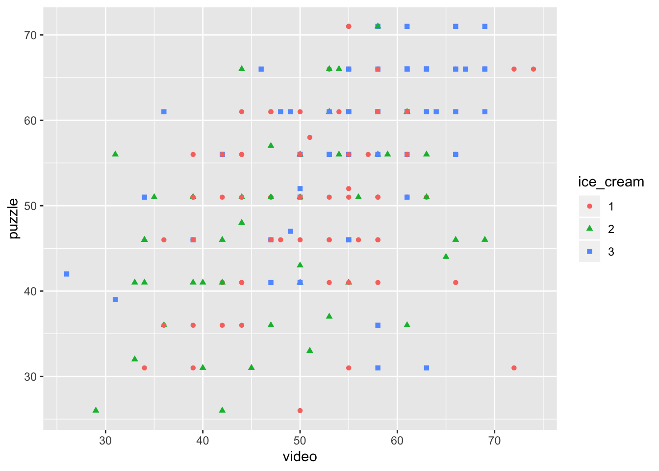
| Version | Author | Date |
|---|---|---|
| 69adea1 | statslee | 2019-09-06 |
How about mark it by gender
icecream$female=as.factor(icecream$female)

p <- ggplot(icecream,aes(x=video, y=puzzle, col=female,shape=female)) +
  geom_point()
p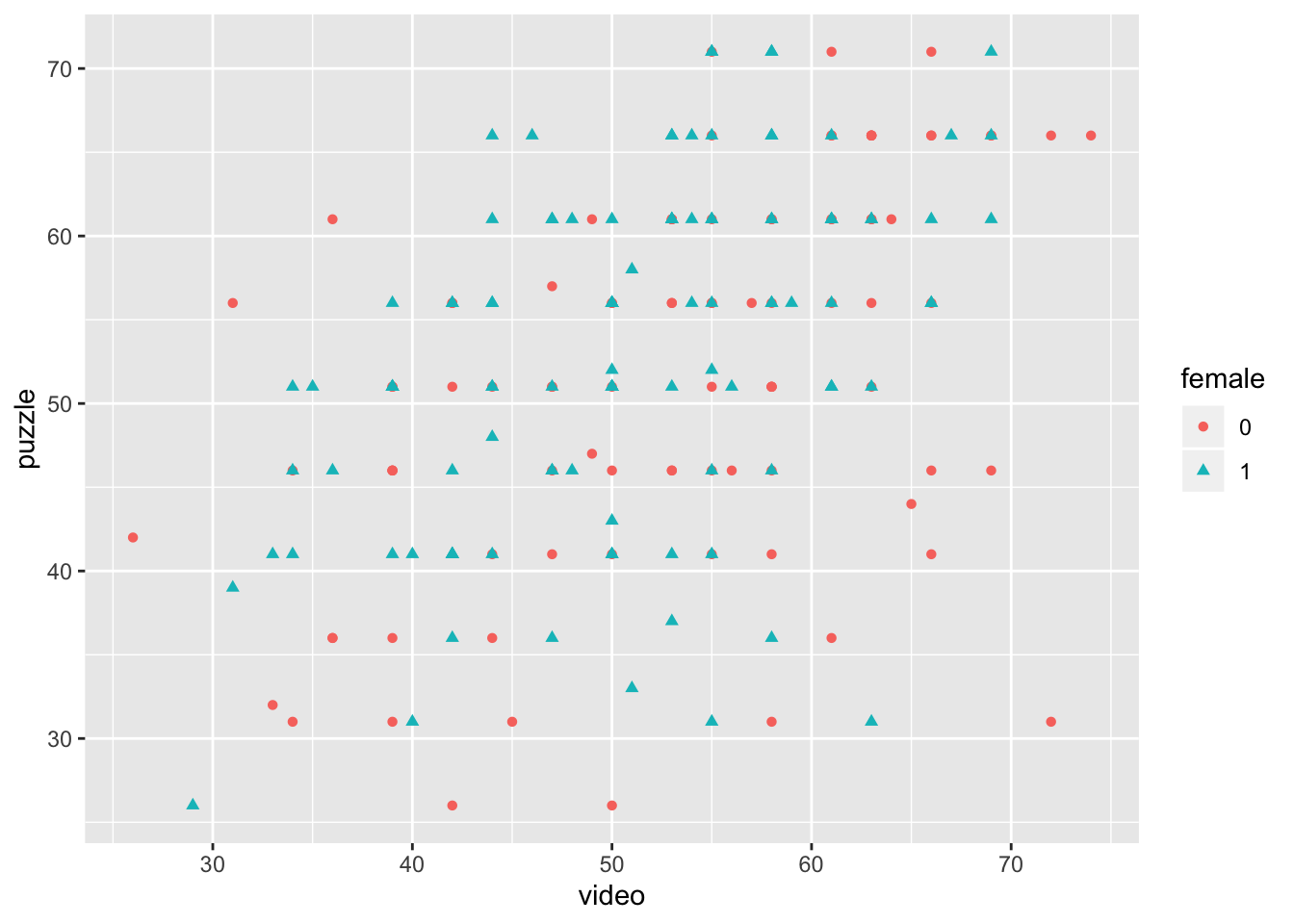
| Version | Author | Date |
|---|---|---|
| 69adea1 | statslee | 2019-09-06 |
p <- ggplot(icecream,aes(x=ice_cream, y=puzzle, col=female,shape=female)) +
  geom_point()
p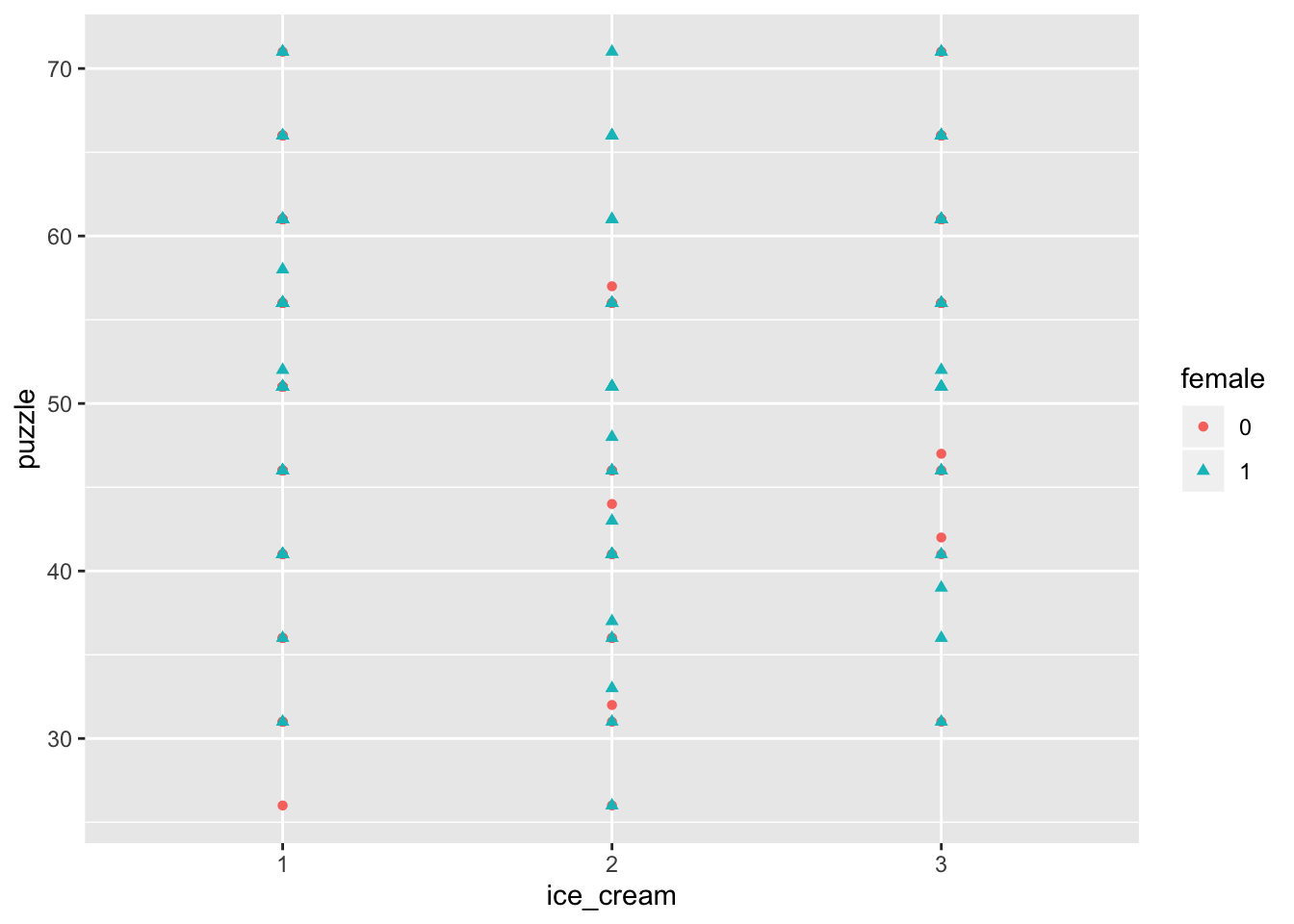
| Version | Author | Date |
|---|---|---|
| 69adea1 | statslee | 2019-09-06 |
Many other ways to customize the plot
p <- ggplot(icecream, aes(x=ice_cream, y=puzzle,fill=ice_cream)) +
  geom_boxplot()
p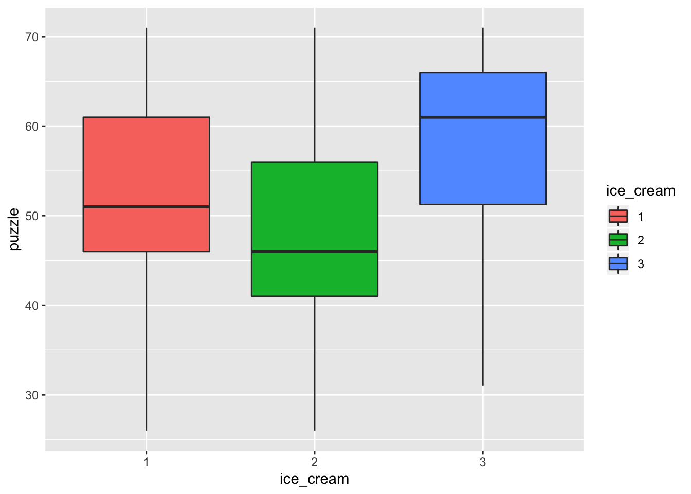
| Version | Author | Date |
|---|---|---|
| 69adea1 | statslee | 2019-09-06 |
p <- ggplot(icecream, aes(x=ice_cream, y=puzzle,fill=female)) +
  geom_boxplot()
p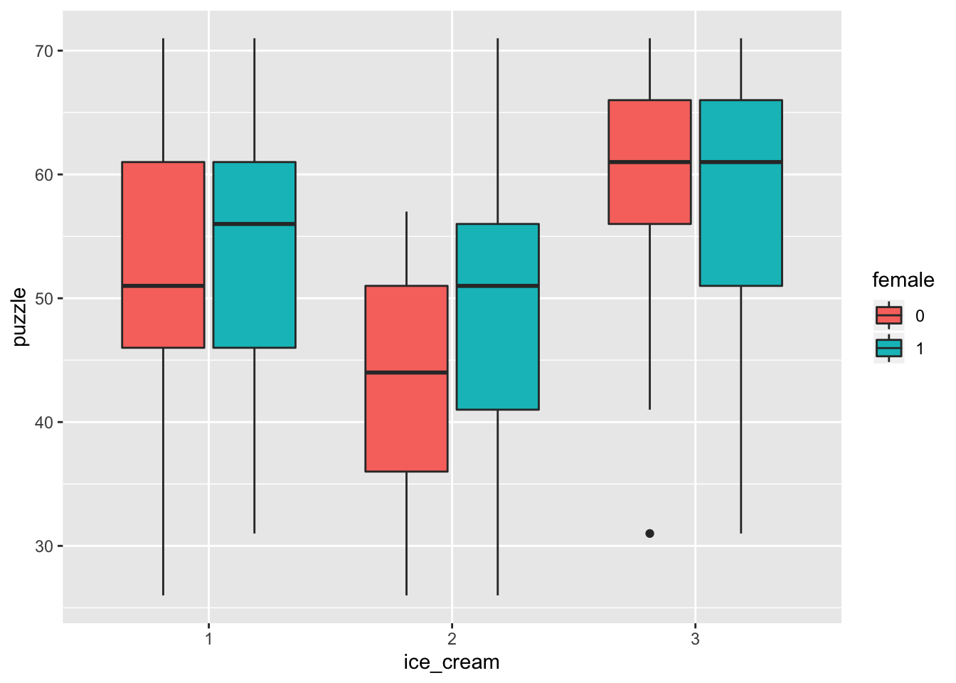
| Version | Author | Date |
|---|---|---|
| 69adea1 | statslee | 2019-09-06 |
p+scale_fill_hue(l=70, c=80) #many other ways to change the color/theme/type, etc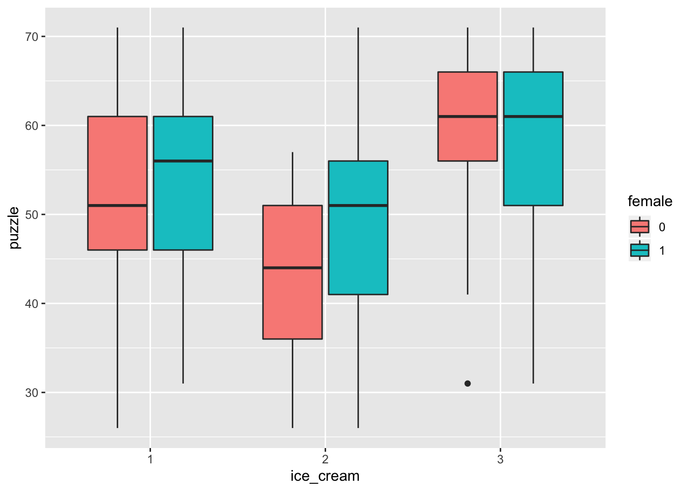
| Version | Author | Date |
|---|---|---|
| 69adea1 | statslee | 2019-09-06 |
Part 3: Simple Linear Regression
copier.fit <- lm(minutes~number,data=copier)
copier.fit
Call:
lm(formula = minutes ~ number, data = copier)

Coefficients:
(Intercept)       number
-0.5802 15.0352 class(copier.fit)[1] "lm"str(copier.fit)List of 12
$ coefficients : Named num [1:2] -0.58 15.04
..- attr(*, "names")= chr [1:2] "(Intercept)" "number"
$ residuals : Named num [1:45] -9.49 0.439 1.474 11.51 -2.455 ...
..- attr(*, "names")= chr [1:45] "1" "2" "3" "4" ...
$ effects : Named num [1:45] -511.61 277.42 2.56 12.5 -1.55 ...
..- attr(*, "names")= chr [1:45] "(Intercept)" "number" "" "" ...
$ rank : int 2
$ fitted.values: Named num [1:45] 29.5 59.6 44.5 29.5 14.5 ...
..- attr(*, "names")= chr [1:45] "1" "2" "3" "4" ...
$ assign : int [1:2] 0 1
$ qr :List of 5
..$ qr : num [1:45, 1:2] -6.708 0.149 0.149 0.149 0.149 ...
.. ..- attr(*, "dimnames")=List of 2
.. .. ..$ : chr [1:45] "1" "2" "3" "4" ...
.. .. ..$ : chr [1:2] "(Intercept)" "number"
.. ..- attr(*, "assign")= int [1:2] 0 1
..$ qraux: num [1:2] 1.15 1.04
..$ pivot: int [1:2] 1 2
..$ tol : num 1e-07
..$ rank : int 2
..- attr(*, "class")= chr "qr"
$ df.residual : int 43
$ xlevels : Named list()
$ call : language lm(formula = minutes ~ number, data = copier)
$ terms :Classes 'terms', 'formula' language minutes ~ number
.. ..- attr(*, "variables")= language list(minutes, number)
.. ..- attr(*, "factors")= int [1:2, 1] 0 1
.. .. ..- attr(*, "dimnames")=List of 2
.. .. .. ..$ : chr [1:2] "minutes" "number"
.. .. .. ..$ : chr "number"
.. ..- attr(*, "term.labels")= chr "number"
.. ..- attr(*, "order")= int 1
.. ..- attr(*, "intercept")= int 1
.. ..- attr(*, "response")= int 1
.. ..- attr(*, ".Environment")=<environment: R_GlobalEnv>
.. ..- attr(*, "predvars")= language list(minutes, number)
.. ..- attr(*, "dataClasses")= Named chr [1:2] "numeric" "numeric"
.. .. ..- attr(*, "names")= chr [1:2] "minutes" "number"
$ model :'data.frame': 45 obs. of 2 variables:
..$ minutes: int [1:45] 20 60 46 41 12 137 68 89 4 32 ...
..$ number : int [1:45] 2 4 3 2 1 10 5 5 1 2 ...
..- attr(*, "terms")=Classes 'terms', 'formula' language minutes ~ number
.. .. ..- attr(*, "variables")= language list(minutes, number)
.. .. ..- attr(*, "factors")= int [1:2, 1] 0 1
.. .. .. ..- attr(*, "dimnames")=List of 2
.. .. .. .. ..$ : chr [1:2] "minutes" "number"
.. .. .. .. ..$ : chr "number"
.. .. ..- attr(*, "term.labels")= chr "number"
.. .. ..- attr(*, "order")= int 1
.. .. ..- attr(*, "intercept")= int 1
.. .. ..- attr(*, "response")= int 1
.. .. ..- attr(*, ".Environment")=<environment: R_GlobalEnv>
.. .. ..- attr(*, "predvars")= language list(minutes, number)
.. .. ..- attr(*, "dataClasses")= Named chr [1:2] "numeric" "numeric"
.. .. .. ..- attr(*, "names")= chr [1:2] "minutes" "number"
- attr(*, "class")= chr "lm"summary(copier.fit)
Call:
lm(formula = minutes ~ number, data = copier)

Residuals:
     Min       1Q   Median       3Q      Max
-22.7723  -3.7371   0.3334   6.3334  15.4039

Coefficients:
            Estimate Std. Error t value Pr(>|t|)
(Intercept)  -0.5802     2.8039  -0.207    0.837
number       15.0352     0.4831  31.123   <2e-16 ***
---
Signif. codes:  0 '***' 0.001 '**' 0.01 '*' 0.05 '.' 0.1 ' ' 1

Residual standard error: 8.914 on 43 degrees of freedom
Multiple R-squared:  0.9575,    Adjusted R-squared:  0.9565
F-statistic: 968.7 on 1 and 43 DF,  p-value: < 2.2e-16
plot(minutes~number, data=copier)
abline(-0.5802,15.0352)#by definition of the line abline(intercept, slope)
#The following are alternative ways to draw the fitted regression line.
lines(copier$number,-0.5802+15.0352*copier$number)#other way
abline(copier.fit)#simple way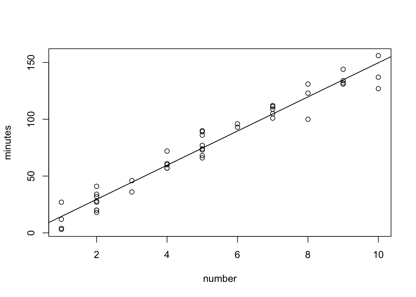
| Version | Author | Date |
|---|---|---|
| 69adea1 | statslee | 2019-09-06 |
#ggplot2
fitted(copier.fit)
1 2 3 4 5 6 7
29.49034 59.56084 44.52559 29.49034 14.45509 149.77232 74.59608
8 9 10 11 12 13 14
74.59608 14.45509 29.49034 134.73708 149.77232 89.63133 44.52559
15 16 17 18 19 20 21
59.56084 119.70183 104.66658 119.70183 149.77232 59.56084 74.59608
22 23 24 25 26 27 28
104.66658 104.66658 74.59608 134.73708 104.66658 29.49034 74.59608
29 30 31 32 33 34 35
104.66658 89.63133 119.70183 74.59608 29.49034 29.49034 14.45509
36 37 38 39 40 41 42
59.56084 74.59608 134.73708 104.66658 14.45509 134.73708 29.49034
43 44 45
29.49034 59.56084 74.59608 copier$fitted=fitted(copier.fit)
p <- ggplot(copier,aes(x=number, y=minutes)) +
geom_point()
p
| Version | Author | Date |
|---|---|---|
| 69adea1 | statslee | 2019-09-06 |
  #geom_line(aes(x=number,y=minutes)) try this and show
  #the function of geom_line
p <- p + geom_line(aes(x=number,y=fitted))
p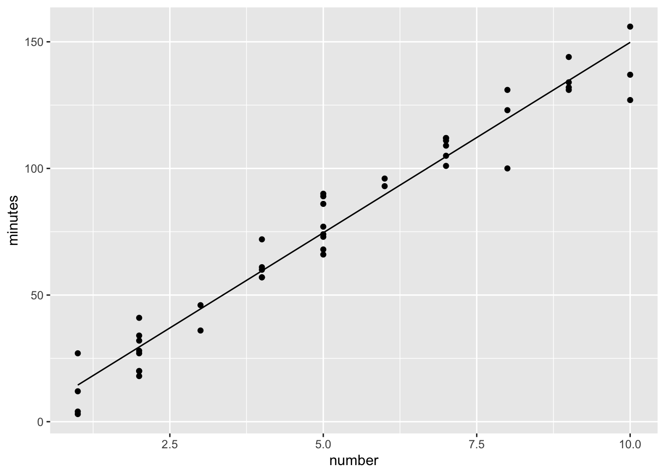
| Version | Author | Date |
|---|---|---|
| 69adea1 | statslee | 2019-09-06 |
sessionInfo()R version 3.6.1 (2019-07-05)
Platform: x86_64-apple-darwin15.6.0 (64-bit)
Running under: macOS Mojave 10.14.6
Matrix products: default
BLAS: /Library/Frameworks/R.framework/Versions/3.6/Resources/lib/libRblas.0.dylib
LAPACK: /Library/Frameworks/R.framework/Versions/3.6/Resources/lib/libRlapack.dylib
locale:
[1] en_US.UTF-8/en_US.UTF-8/en_US.UTF-8/C/en_US.UTF-8/en_US.UTF-8
attached base packages:
[1] stats graphics grDevices utils datasets methods base
other attached packages:
[1] ggplot2_3.2.1 dplyr_0.8.3 workflowr_1.4.0
loaded via a namespace (and not attached):
[1] Rcpp_1.0.2 pillar_1.4.2 compiler_3.6.1 git2r_0.26.1
[5] tools_3.6.1 zeallot_0.1.0 digest_0.6.20 evaluate_0.14
[9] tibble_2.1.3 gtable_0.3.0 pkgconfig_2.0.2 rlang_0.4.0
[13] cli_1.1.0 yaml_2.2.0 xfun_0.9 withr_2.1.2
[17] stringr_1.4.0 knitr_1.24 fs_1.3.1 vctrs_0.2.0
[21] rprojroot_1.3-2 grid_3.6.1 tidyselect_0.2.5 glue_1.3.1
[25] R6_2.4.0 fansi_0.4.0 rmarkdown_1.15 purrr_0.3.2
[29] magrittr_1.5 whisker_0.3-2 backports_1.1.4 scales_1.0.0
[33] htmltools_0.3.6 assertthat_0.2.1 colorspace_1.4-1 labeling_0.3
[37] utf8_1.1.4 stringi_1.4.3 lazyeval_0.2.2 munsell_0.5.0
[41] crayon_1.3.4