EC524: Lab 04

tidymodels Modeling, Resampling, and Prediction

Jose Rojas-Fallas

2026

Lab Agenda

1. Modeling

2. Resampling and Prediction

Preprocessing

A quick catch-up of what we did:

i Loaded credit data, cleaned it up and created our outcome variable

# Setup 
# Load packages
library(pacman)
p_load(tidyverse, modeldata, skimr, janitor, tidymodels, magrittr, visdat)
# Load the credit dataset
data(credit_data)
# (Optional) Assign a new name
credit_df <- credit_data
# 'Fix' names
credit_df %<>% 
    clean_names() %>%
    # Create a dummy variable for 'good' credit status
    mutate(status_good = 1 * (status == "good")) %>%
    # Drop the old status variable
    select(-status)

Preprocessing

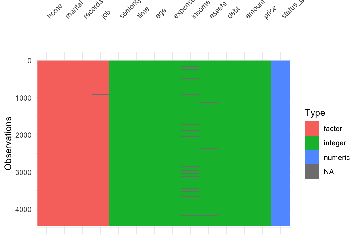
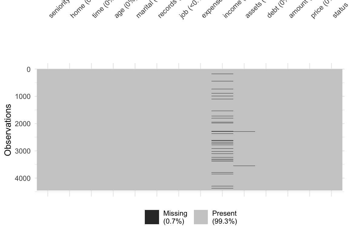
ii Visualized the data and found there is missing data

New way: visdat::vis_dat() and visdat::vis_miss()

# Can use skimr::skim() or a new way to visualize is

credit_df %>% visdat::vis_dat()

credit_df %>% visdat::vis_miss()

Preprocessing

iii Set up a recipe() that helped us clean the data and impute necessary missing data

Note: I am storing the preprocessing steps in an object, that I can call on later

# Define the recipe: status_good predicted by all other variables in credit_df
recipe_all = recipe(status_good ~ ., data = credit_df)
# Putting it all together
preprocessing_steps <- recipe_all %>%
  # Mean imputation for numeric predictors
  step_impute_mean(all_predictors() & all_numeric()) %>% 
  # KNN imputation for categorical predictors
  step_impute_knn(all_predictors() & all_nominal(), neighbors = 5) %>%
  # Create dummies for categorical variables
  step_dummy(all_predictors() & all_nominal()) %>%
  # Interactions
  step_interact(~income:starts_with("home"))

Preprocessing

iv Recall that creating a recipe() with steps are only instructions, we still need to prep() and juice() it to get a dataframe

credit_clean <- preprocessing_steps %>% prep() %>% juice()

Fitting Models

Now that we have a nice clean dataset, we can begin to fit a model

In the tidymodels universe, we need to do (at least) three things:

1. Define the Model Specification

The Type of model we want (linear regression, KNN, or random forest)

2. Define the Engine

The function/package that R will use to fit your model

3. Define the data and relationships to fit

Point R to your data and define output/input

Specifying the Type of Model

Your first decision is the type of model you want to use (in tidymodels “type” = “specification”, but that may be confusing for the econometric mind)

You have many choices for the type of model you want to specify. Each comes with a different parsnip function
- Linear Regression: linear_reg()
- K-Nearest Neighbor: nearest_neighbor()
- Random Forest: rand_forest()
We can check what the linear regression model function linear_reg() tells us:

linear_reg()

Linear Regression Model Specification (regression)

Computational engine: lm

Setting an Engine

Before we actually fit/train the model, we need to tell R which engine we want to use.

The engine tells R what algorithms to use, and some algos may differ greatly from others

You define the engine using the set_engine() function

You can see that we can fit a linear regression model using any of five engines

"lm"
"glmnet"
"stan"

"spark"
"keras"

You can use show_engines() function to see which engines are available for your model type

# Show which engines are available for linear_reg()
show_engines("linear_reg")

# A tibble: 8 × 2
  engine   mode               
  <chr>    <chr>              
1 lm       regression         
2 glm      regression         
3 glmnet   regression         
4 stan     regression         
5 spark    regression         
6 keras    regression         
7 brulee   regression         
8 quantreg quantile regression

Setting an Engine

We will use the "lm" engine to fit a traditional linear regression model. Fancy stuff comes later.

# Define the "lm" engine for `linear_reg()`
linear_reg() %>% set_engine("lm")

Linear Regression Model Specification (regression)

Computational engine: lm

Setting an Engine

We can also use translate() to see what is going on under the hood a bit more

# Translate our regression model
linear_reg() %>% set_engine("lm") %>% translate()

Linear Regression Model Specification (regression)

Computational engine: lm 

Model fit template:
stats::lm(formula = missing_arg(), data = missing_arg(), weights = missing_arg())

Fitting (Training) Your Model

After defining the type of model and the engine, we can now begin to fit() the model

The fit() function wants a few arguments
- The model_spec object comes from setting the type and engine (form before)
- A formula the defines the outputs and inputs (just like using lm())
- The data
In our case, we will have:
- Model type is linear_reg() and our Engine is "lm"
- The formula is our linear regression where status_good is our outcome and the other vars. (.) are the predictors
- Our data is our cleaned dataset credit_clean

This is a simple linear regression but the tidymodels way.

est_reg <- 
    # Model Type
    linear_reg() %>%
    # Engine 
    set_engine("lm") %>%
    # Formula 
    fit(status_good ~ ., data = credit_clean)

`tidymodels` Linear Regression

We can use tidy() to see the results in a more usual way

est_reg %>% tidy()

# A tibble: 28 × 5
   term           estimate   std.error statistic  p.value
   <chr>             <dbl>       <dbl>     <dbl>    <dbl>
 1 (Intercept)  0.686      0.175           3.91  9.26e- 5
 2 seniority    0.00927    0.000880       10.5   1.19e-25
 3 time        -0.0000822  0.000473       -0.174 8.62e- 1
 4 age         -0.00153    0.000720       -2.12  3.37e- 2
 5 expenses    -0.00212    0.000376       -5.63  1.95e- 8
 6 income       0.00125    0.000981        1.27  2.03e- 1
 7 assets       0.00000249 0.000000559     4.46  8.53e- 6
 8 debt        -0.0000175  0.00000489     -3.58  3.42e- 4
 9 amount      -0.000234   0.0000207     -11.3   2.21e-29
10 price        0.0000899  0.0000142       6.33  2.70e-10
# ℹ 18 more rows

We can also use this information and use predict() as we have before.

Changing The Type of Model

Okay, so we have just gone through a complex way to run a simple regression model that you likely knew how to do in a simpler way

But the power of tidymodels is coming from its flexibility.

It is very easy to change any of our decisions along the way

Let’s say instead we wanted to fit a KNN model. We just need to change the type of model and engine.

Note Some methods like KNN can be used for either "regression" tasks and "classification" tasks. We want to se the mode for these methods, either within the nearest_neighbor() function (nearest_neighbor(mode = "regression)) or using the set_mode() function.

We can finally choose a value for our parameters (tuning and CV later). In KNN that is just setting a value of \(k\). I’ll arbitrarily choose 6.

est_knn <- nearest_neighbor(mode = "regression", neighbors = 6) %>%
    set_engine("kknn") %>%
    fit(status_good ~ ., data = credit_clean)

est_knn %>% class()

[1] "_train.kknn" "model_fit"

Resampling, Tuning, and Validating

We have omitted a big part of the ML Process: Tuning and Validating models.

As always, we begin with the setup (mostly in case this is not the same week as the other parts)

# Packages
library(pacman)
p_load(tidyverse, modeldata, skimr, janitor, tidymodels, magrittr)
# Load credit data
data(credit_data)
credit_df <- credit_data
# Clean up names
credit_df %<>% clean_names()
# Create a dummy variable for our outcome (good credit status)
credit_df %<>% mutate(status_good = 1 * (status == "good")) %>%
    # drop old status variable
    select(-status)

Simple Sample Splitting

First simple task: Split the full credit_df dataset into a training (sub)set and a testing (sub)set

To split the sample, lets use the initial_split() function from the rsample package.

It splits a proportion (prop argument) of your data into a training subset and leaves the rest for the testing subset.
- If you wanted to sample by strata you could as well
It is another tool for you to use (we had used sample_frac() previously)
The output is an rsplit object, not a dataframe
- We will pass the object given by initial_split() to the training() and testing() functions to get the actual subsets as dataframes

[Note: It can be helpful to set a seed before you split the data for reproducing results]

Simple Sample Splitting

# Set the seed
set.seed(123)
# Create the split (80-20 split)
credit_split <- credit_df %>%
    initial_split(prop = 0.8)
# Check the output
credit_split

<Training/Testing/Total>
<3563/891/4454>

Now we can impose the split by using the training() and testing() functions.

Simple Sample Splitting

After we grab the proper split data, we can check the dimensions to make sure it makes sense

# Grab the training data (Larger Chunk)
credit_train <- credit_split %>% training()
# Grab the testing data (Smaller Chunk)
credit_test <- credit_split %>% testing()
# Check dimensions
dim(credit_df); dim(credit_train); dim(credit_test)

[1] 4454   14

[1] 3563   14

[1] 891  14

Resampling

As you’ve seen in class, the goal of prediction exercises is good out-of-sample performance

To avoid overfitting, while still allowing for “optimal” flexibility, we use resampling methods.

We will use the vfold_cv() function to set up 5-fold cross validation for our model

vfold_cv() takes the following arguments:

data
v, the number of folds
repeats the number of times you want to repeat the cross validation (default is 1)
strata is an optional variable to use for stratified sampling in the folds

Creating the folds looks like:

# set seed
set.seed(123)
# 5-fold CV on the training dataset
credit_cv <- credit_train %>% vfold_cv(v = 5)
# Check the output 
credit_cv %>% tidy()

# A tibble: 17,815 × 3
     Row Data     Fold 
   <int> <chr>    <chr>
 1     1 Analysis Fold1
 2     1 Analysis Fold2
 3     1 Analysis Fold4
 4     1 Analysis Fold5
 5     2 Analysis Fold2
 6     2 Analysis Fold3
 7     2 Analysis Fold4
 8     2 Analysis Fold5
 9     3 Analysis Fold1
10     3 Analysis Fold3
# ℹ 17,805 more rows

Define the Data-Processing Recipe

For each split, we want to process the data (recipes) and fit the model (parsnip)

Important! We want to preprocess the training subset in each split separately from the split’s subset. This helps us avoid data leakage.

In everything we have done before, we impute using the entire data. We are supposed to be keeping them totally separate.

What we really want is to process the datasets independently, but using the same recipe and steps

Define the Recipe

Only the recipe, no prep(), juice(), or bake()

# Data-processing recipe
    # IMPORTANT! NOTICE I AM USING THE TRAINING DATA HERE NOT THE FULL SAMPLE
credit_recipe <- recipe(status_good ~ ., data = credit_train) %>%
    # Mean imputation for numeric predictors
    step_impute_mean(all_predictors() & all_numeric()) %>% 
    # KNN imputation for categorical predictors
    step_impute_knn(all_predictors() & all_nominal(), neighbors = 5) %>%
    # Create dummies for categorical variables
    step_dummy(all_predictors() & all_nominal()) %>%
    # Interactions
    step_interact(~income:starts_with("home"))
# Check the result
credit_recipe

── Recipe ──────────────────────────────────────────────────────────────────────

── Inputs

Number of variables by role

outcome:    1
predictor: 13

── Operations

• Mean imputation for: all_predictors() & all_numeric()

• K-nearest neighbor imputation for: all_predictors() & all_nominal()

• Dummy variables from: all_predictors() & all_nominal()

• Interactions with: income:starts_with("home")

Define the Model

Tell it both the type of model and the desired engine

Keeping it simple with linear_reg() and the standard "lm"

Feel free to try whatever you want here in the code to test things out

Although not necessary for "lm", we will set the mode using set_mode(). Just good to get into the habit of things

model_lm <- 
    # Set my model
    linear_reg() %>%
    # Set my mode
    set_mode("regression") %>%
    # Set my engine
    set_engine("lm")
# Check the result
model_lm

Linear Regression Model Specification (regression)

Computational engine: lm

Putting it Together in a Workflow

We have three different objects floating around

The defined CV splits for the training dataset (credit_cv)
The recipe for processing the data (credit_recipe)
The model that we want to fit on the trianing data (folds)

Now we need to put them together.

Repeating the preprocessing for each training and validation split could be annoying if you did it all by hand.
Luckily, we will be uwing the workflows package within tidymodels

How? Literally by defining a workflow with the workflow() function and then pipe in your model and then recipe

workflow() %>% 
    add_model(model_lm) %>%
    add_recipe(credit_recipe)

══ Workflow ════════════════════════════════════════════════════════════════════
Preprocessor: Recipe
Model: linear_reg()

── Preprocessor ────────────────────────────────────────────────────────────────
4 Recipe Steps

• step_impute_mean()
• step_impute_knn()
• step_dummy()
• step_interact()

── Model ───────────────────────────────────────────────────────────────────────
Linear Regression Model Specification (regression)

Computational engine: lm

Putting it Together in a Workflow

The workflow we just wrote defines the model, the data processing, and the engine.

We will have a couple of options:

1. Fit a Single Model Without CV

2. Fit a Single Model With CV

3. Tune your model (using CV)

Putting it Together in a Workflow

The workflow we just wrote defines the model, the data processing, and the engine.

1. Fit a Single Model Without CV

If you only want to fit the model (with no CV), you can pipe the workflow to fit(data = dataframe)

This is not what we will ultimately want as we want to cross-validate using the folds we created

# Workflow and model fit
workflow() %>%
    add_model(model_lm) %>%
    add_recipe(credit_recipe) %>%
    fit(data = credit_df)

══ Workflow [trained] ══════════════════════════════════════════════════════════
Preprocessor: Recipe
Model: linear_reg()

── Preprocessor ────────────────────────────────────────────────────────────────
4 Recipe Steps

• step_impute_mean()
• step_impute_knn()
• step_dummy()
• step_interact()

── Model ───────────────────────────────────────────────────────────────────────

Call:
stats::lm(formula = ..y ~ ., data = data)

Coefficients:
          (Intercept)              seniority                   time  
            6.855e-01              9.267e-03             -8.311e-05  
                  age               expenses                 income  
           -1.525e-03             -2.120e-03              1.250e-03  
               assets                   debt                 amount  
            2.493e-06             -1.750e-05             -2.344e-04  
                price             home_other             home_owner  
            8.991e-05              6.054e-02              2.588e-01  
         home_parents              home_priv              home_rent  
            2.135e-01              1.559e-01              7.157e-02  
      marital_married      marital_separated         marital_single  
            7.142e-02             -1.320e-01              8.053e-03  
        marital_widow            records_yes          job_freelance  
            1.179e-02             -2.969e-01             -1.174e-01  
           job_others            job_partime    income_x_home_other  
           -1.341e-01             -2.979e-01             -4.669e-04  
  income_x_home_owner  income_x_home_parents     income_x_home_priv  
           -5.550e-04             -4.636e-04             -5.933e-04  
   income_x_home_rent  
           -5.508e-05

Putting it Together in a Workflow

The workflow we just wrote defines the model, the data processing, and the engine.

2. Fit a Single Model With CV

If you want to estimate your model’s out-of-sample performance, then you can use fit_resamples() And we can use collect_metrics() function to assess the performance across the resamples

By default, it will average across the folds (notice it says n = 5, which is our folds).

fit_lm_cv <- 
    workflow() %>%
    add_model(model_lm) %>%
    add_recipe(credit_recipe) %>%
    fit_resamples(credit_cv)
# Check performance
fit_lm_cv %>% collect_metrics()

# A tibble: 2 × 6
  .metric .estimator  mean     n std_err .config        
  <chr>   <chr>      <dbl> <int>   <dbl> <chr>          
1 rmse    standard   0.390     5 0.00428 pre0_mod0_post0
2 rsq     standard   0.255     5 0.0163  pre0_mod0_post0

Putting it Together in a Workflow

The workflow we just wrote defines the model, the data processing, and the engine.

2. Fit a Single Model With CV

If you wanted to see how the model performs on each fold then you can set summarize = F inside collect_metrics()

fit_lm_cv %>% collect_metrics(summarize = F)

# A tibble: 10 × 5
   id    .metric .estimator .estimate .config        
   <chr> <chr>   <chr>          <dbl> <chr>          
 1 Fold1 rmse    standard       0.393 pre0_mod0_post0
 2 Fold1 rsq     standard       0.257 pre0_mod0_post0
 3 Fold2 rmse    standard       0.387 pre0_mod0_post0
 4 Fold2 rsq     standard       0.255 pre0_mod0_post0
 5 Fold3 rmse    standard       0.377 pre0_mod0_post0
 6 Fold3 rsq     standard       0.308 pre0_mod0_post0
 7 Fold4 rmse    standard       0.391 pre0_mod0_post0
 8 Fold4 rsq     standard       0.246 pre0_mod0_post0
 9 Fold5 rmse    standard       0.404 pre0_mod0_post0
10 Fold5 rsq     standard       0.206 pre0_mod0_post0

Putting it Together in a Workflow

RMSE and \(R^{2}\) are the default metrics. We can change them using the metrics argument inside of fit_resamples()

You can pass whichever metric you want to use from the yardstick package.

Suppose we want Mean Absolute Error (MAE) as well

# Define Workflow, then fit model on folds
fit_lm_cv <- 
    workflow() %>%
    add_model(model_lm) %>%
    add_recipe(credit_recipe) %>%
    fit_resamples(credit_cv, metrics = metric_set(rmse, rsq, mae))
# Check performance
fit_lm_cv %>% collect_metrics()

# A tibble: 3 × 6
  .metric .estimator  mean     n std_err .config        
  <chr>   <chr>      <dbl> <int>   <dbl> <chr>          
1 mae     standard   0.320     5 0.00386 pre0_mod0_post0
2 rmse    standard   0.390     5 0.00428 pre0_mod0_post0
3 rsq     standard   0.255     5 0.0163  pre0_mod0_post0

Putting it Together in a Workflow

The workflow we just wrote defines the model, the data processing, and the engine.

3. Tune your model (using CV)

Instead of “just” estimating out-of-sample model performance for a specified model and pre-processing operations, we will often want to tune a model’s hyperparameter(s)

Suppose we are using \(k\) nearest neighbors instead of a linear regression. Then we either need to specify a \(k\) or we need to tune k.

By tune we mean estimate the out-of-sample performance for various values of \(k\) and then choose the “best” \(k\) (based on some metric that defines “best”).

To begin, let’s define a KNN model using nearest_neighbor(). We will tell it to tune by specifiying we want to tune() as our neighbors value.

# Define our KNN Model
model_knn <- 
    nearest_neighbor(neighbors = tune()) %>%
    set_mode("regression") %>%
    set_engine("kknn") 
# Check the Model
model_knn

K-Nearest Neighbor Model Specification (regression)

Main Arguments:
  neighbors = tune()

Computational engine: kknn

Tuning KNN

Almost ready to fit the model, but we still need to let R know which values to try for the parameter we are tuning

To tune our hyperparameter(s), we will use the tune_grid() function (instead of fit() or fit_resamples() functions)

tune_grid() works similarly to fit_resamples() except it takes an additional argument: grid

We will pass the possible values of our hyperparameter(s) to the grid argument and it will evaluate each fold of our samples on each set of hyperparameter(s) we fed it

Tuning KNN

KNN only needs one hyperparameter: neighbors. We can give the grid argument a data.frame of all the values we would like to try, where the column’s name matches the hyperparameter we are trying to tune neighbors

If, like me, you don’t know what may be “reasonable” values, you can see what is suggested by the function with the same name as the hyperparameter (neighbors() in this case)

# Check "suggested" value of neighbors
neighbors()

Tuning KNN

Caution

As you add more values of hyperparameters, you fit more models.

More models means more computation.

More computation means more time.

Keep in mind that you are already fitting a model on each fold (5 in our example) so if you want to test 100 values of neighbors then you need to fit \(100 \times 5\) models

Let’s try 1 neighbor (surely not the best) and then 5, and then 10 to 100 by 10s

Tuning KNN

Let’s try 1 neighbor (surely not the best) and then 5, and then 10 to 100 by 10s

# Define the workflow
workflow_knn <- workflow() %>%
    add_model(model_knn) %>%
    add_recipe(credit_recipe)

# Fit the workflow on our predefined folds and hyperparameters
fit_knn_cv <- workflow_knn %>%
    tune_grid(
        # CV data
        credit_cv, 
        # Grid where we put our values
        grid = data.frame(neighbors = c(1, 5, seq(10,100,10))),
        metrics = metric_set(rmse, rsq, mae)
    )

# Check performance
fit_knn_cv %>% collect_metrics()

# A tibble: 36 × 7
   neighbors .metric .estimator   mean     n std_err .config         
       <dbl> <chr>   <chr>       <dbl> <int>   <dbl> <chr>           
 1         1 mae     standard   0.298      5 0.00884 pre0_mod01_post0
 2         1 rmse    standard   0.546      5 0.00808 pre0_mod01_post0
 3         1 rsq     standard   0.0706     5 0.00940 pre0_mod01_post0
 4         5 mae     standard   0.301      5 0.00667 pre0_mod02_post0
 5         5 rmse    standard   0.449      5 0.00632 pre0_mod02_post0
 6         5 rsq     standard   0.129      5 0.0130  pre0_mod02_post0
 7        10 mae     standard   0.304      5 0.00520 pre0_mod03_post0
 8        10 rmse    standard   0.424      5 0.00488 pre0_mod03_post0
 9        10 rsq     standard   0.160      5 0.0126  pre0_mod03_post0
10        20 mae     standard   0.308      5 0.00469 pre0_mod04_post0
# ℹ 26 more rows

Tuning KNN

Recognize what we just did was pretty cool: We changed very little to move from a cross-validated regression model to a CV-tuned KNN model.

The output is also cool, but overwhelming.

We can use the show_best() function to have it tell us which value(s) of the hyperparameters performed best according to the metrics we asked for. We either need to give show_best() the name of the metric to use, or it will choose one for us.

show_best() also defaults to showing the top 5 models but you can change that with the n argument
select_best() allows us to select the best model (based on the metrics)

# Show the best model in terms of RMSE
fit_knn_cv %>% show_best(metric = "rmse",, n = 5)

# A tibble: 5 × 7
  neighbors .metric .estimator  mean     n std_err .config         
      <dbl> <chr>   <chr>      <dbl> <int>   <dbl> <chr>           
1        60 rmse    standard   0.404     5 0.00261 pre0_mod08_post0
2        70 rmse    standard   0.404     5 0.00245 pre0_mod09_post0
3        50 rmse    standard   0.404     5 0.00283 pre0_mod07_post0
4        80 rmse    standard   0.404     5 0.00232 pre0_mod10_post0
5        40 rmse    standard   0.404     5 0.00315 pre0_mod06_post0

# Show the best model in terms of RMSE
fit_knn_cv %>% show_best(metric = "rsq", n = 3)

# A tibble: 3 × 7
  neighbors .metric .estimator  mean     n std_err .config         
      <dbl> <chr>   <chr>      <dbl> <int>   <dbl> <chr>           
1       100 rsq     standard   0.210     5  0.0105 pre0_mod12_post0
2        90 rsq     standard   0.210     5  0.0105 pre0_mod11_post0
3        80 rsq     standard   0.209     5  0.0105 pre0_mod10_post0

We Can Visualize It

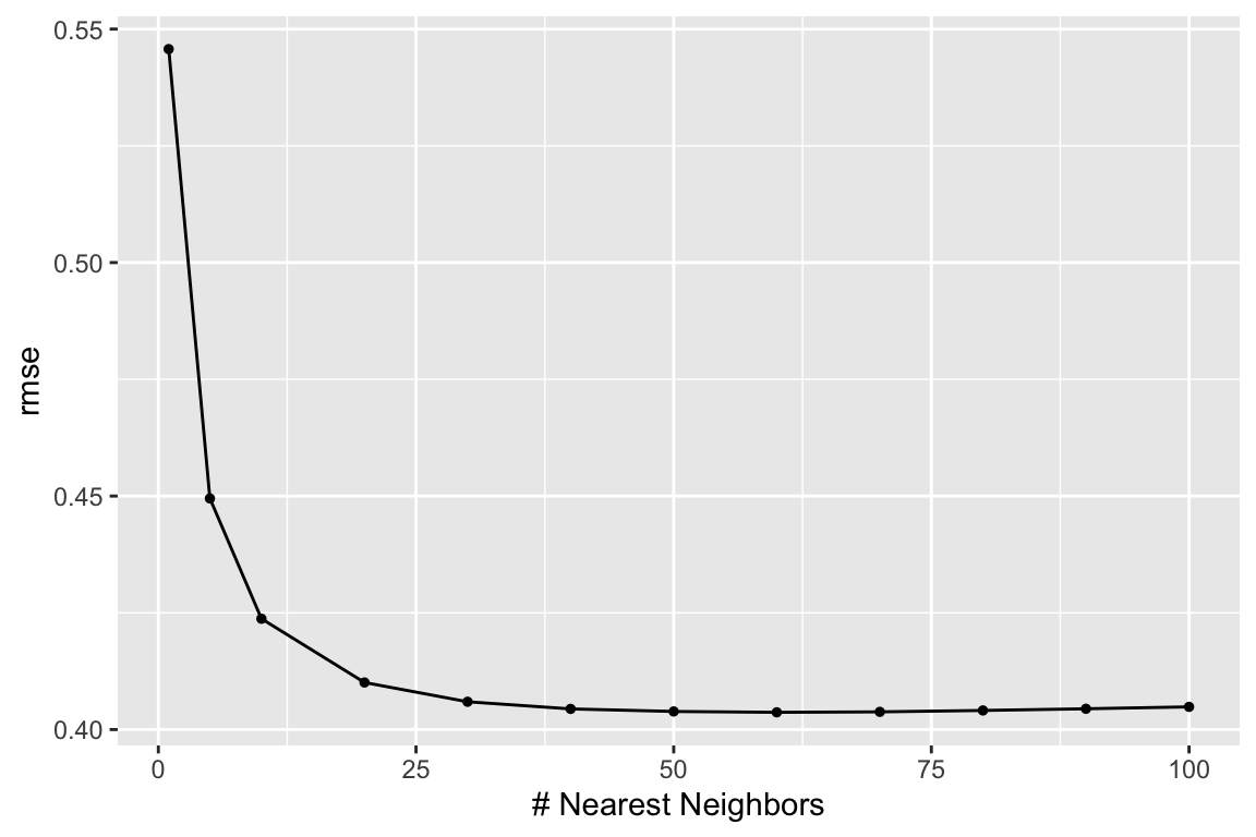
We can use the autoplot() function for a nice and quick picture (we can improve on it too).

We just need to tell it what metric we want to map.

# Quick plot
autoplot(fit_knn_cv, metric = "rmse")

Visualize it Part 02

# Plot metrics' averages across values of 'k'
fit_knn_cv %>% 
    collect_metrics(summarize = T) %>%
    ggplot(aes(x = neighbors, y = mean)) +
    geom_line(size = 0.7, alpha = 0.6) +
    geom_point(size = 2.5) +
    facet_wrap(~ toupper(.metric), scales = "free", nrow = 1) +
    scale_x_continuous("Neighbors (k)", labels = scales::label_number()) +
    scale_y_continuous("Estimate") +
    scale_color_viridis_d("CV Folds:") +
    theme_minimal() + 
    theme(legend.position = "bottom")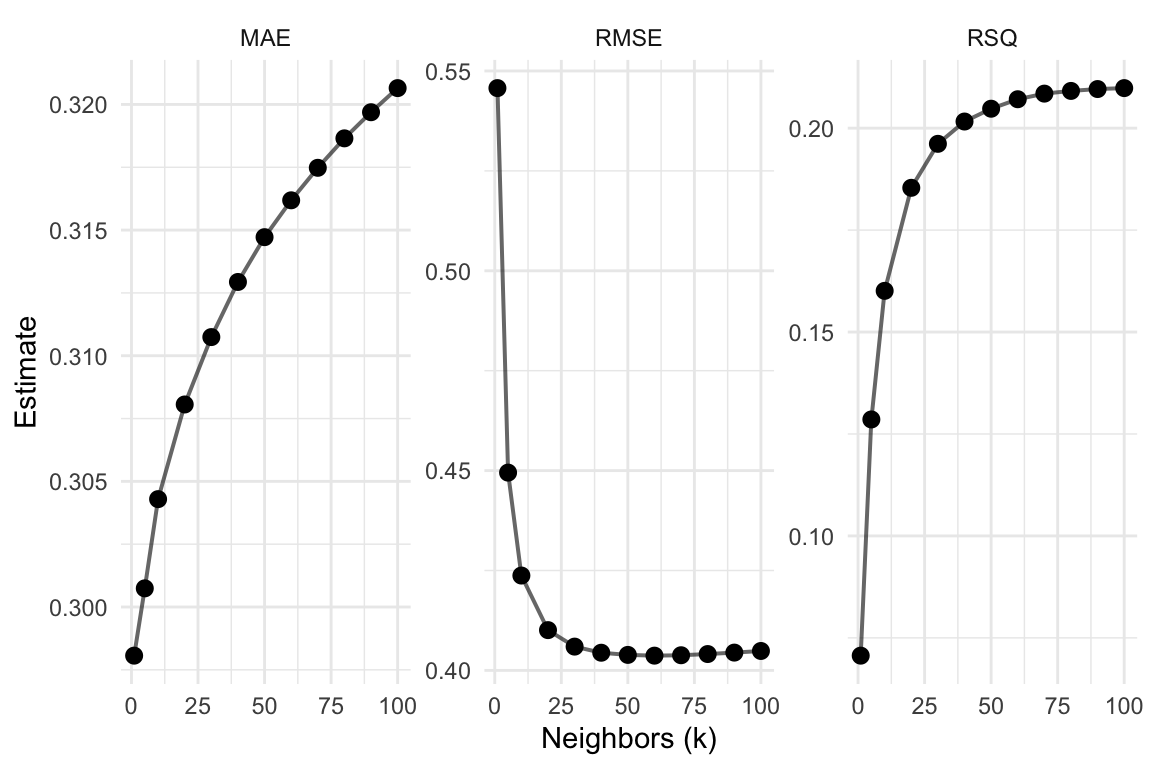

Visualize it Part 03

# Show each fold's metrics across values of 'k'
fit_knn_cv %>% 
    collect_metrics(summarize = F) %>%
    ggplot(aes(x = neighbors, y = .estimate, color = id)) +
    geom_line(size = 0.7, alpha = 0.6) +
    geom_point(size = 2.5) +
    facet_wrap(~ toupper(.metric), scales = "free", nrow = 1) +
    scale_x_continuous("Neighbors (k)", labels = scales::label_number()) +
    scale_y_continuous("Estimate") +
    scale_color_viridis_d("CV Folds:") +
    theme_minimal() + 
    theme(legend.position = "bottom")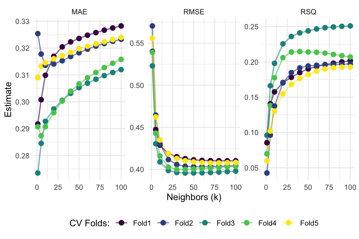

Lastly: Prediction!

We are just about finished

We will wrap it up by taking our selected model (the best model), fitting it on all of the training data, and then predict onto the test data

Recall we pick our “best” model (using whatever metric we prefer) using the select_best() function

Once we found the “best” model, we wrap up our workflow() using finalize_workflow()

This function wants (1) your initial workflow and (2) your best model

# The final workflow for our KNN model
final_knn <-
    workflow_knn %>% 
    finalize_workflow(select_best(fit_knn_cv, metric = "rmse"))
# Check out the final workflow object
final_knn

══ Workflow ════════════════════════════════════════════════════════════════════
Preprocessor: Recipe
Model: nearest_neighbor()

── Preprocessor ────────────────────────────────────────────────────────────────
4 Recipe Steps

• step_impute_mean()
• step_impute_knn()
• step_dummy()
• step_interact()

── Model ───────────────────────────────────────────────────────────────────────
K-Nearest Neighbor Model Specification (regression)

Main Arguments:
  neighbors = 60

Computational engine: kknn

Prediction

Now we fit this finalized workflow to the full training dataset (credit_train).

Enter fit().

# Fitting our final workflow
final_fit_knn <- final_knn %>% fit(data = credit_train)
# Examine the final workflow
final_fit_knn

══ Workflow [trained] ══════════════════════════════════════════════════════════
Preprocessor: Recipe
Model: nearest_neighbor()

── Preprocessor ────────────────────────────────────────────────────────────────
4 Recipe Steps

• step_impute_mean()
• step_impute_knn()
• step_dummy()
• step_interact()

── Model ───────────────────────────────────────────────────────────────────────

Call:
kknn::train.kknn(formula = ..y ~ ., data = data, ks = min_rows(60,     data, 5))

Type of response variable: continuous
minimal mean absolute error: 0.3129085
Minimal mean squared error: 0.1606585
Best kernel: optimal
Best k: 60

Prediction

Finally, we predict onto the testing data by using predict()

# Predict onto the test data
test_hat <- final_fit_knn %>% predict(new_data = credit_test)
# Check out predictions
test_hat %>% head()

# A tibble: 6 × 1
  .pred
  <dbl>
1 0.955
2 0.940
3 0.952
4 0.290
5 0.919
6 0.957

Prediction but Easier

Once we have a final workflow (final_knn is the workflow plus the selected best model), you can pass it to the last_fit() function

Along with the initial split (credit_split in our case) to both:

Fit your final model on your full training dataset
Make predictions onto the testing dataset (defined by the initial split object)

This last_fit() approach streamlines your work and also lets you easily collect metrics using the collect_metrics() function from before

# Write over 'final_fit_knn' with this last_fit() approach
final_fit_knn <- final_knn %>% last_fit(credit_split)
# Collect metrics on the test data!
final_fit_knn %>% collect_metrics()

# A tibble: 2 × 4
  .metric .estimator .estimate .config        
  <chr>   <chr>          <dbl> <chr>          
1 rmse    standard       0.392 pre0_mod0_post0
2 rsq     standard       0.225 pre0_mod0_post0

Prediction but Easier

If instead you want predictions, just use the collect_predictions() on the output from last_fit()

# Get test-sample predictions
final_fit_knn %>% collect_predictions() %>% head()

# A tibble: 6 × 5
  .pred id               status_good  .row .config        
  <dbl> <chr>                  <dbl> <int> <chr>          
1 0.955 train/test split           1     6 pre0_mod0_post0
2 0.940 train/test split           1     8 pre0_mod0_post0
3 0.952 train/test split           1    16 pre0_mod0_post0
4 0.290 train/test split           0    23 pre0_mod0_post0
5 0.919 train/test split           1    24 pre0_mod0_post0
6 0.957 train/test split           1    28 pre0_mod0_post0

EC524: Lab 04

Lab Agenda

Preprocessing

Preprocessing

Preprocessing

Preprocessing

Fitting Models

Specifying the Type of Model

Setting an Engine

Setting an Engine

Setting an Engine

Fitting (Training) Your Model

tidymodels Linear Regression

Changing The Type of Model

Resampling, Tuning, and Validating

Simple Sample Splitting

Simple Sample Splitting

Simple Sample Splitting

Resampling

Define the Data-Processing Recipe

Define the Recipe

Define the Model

Putting it Together in a Workflow

Putting it Together in a Workflow

Putting it Together in a Workflow

Putting it Together in a Workflow

Putting it Together in a Workflow

Putting it Together in a Workflow

Putting it Together in a Workflow

Tuning KNN

Tuning KNN

Tuning KNN

Tuning KNN

Tuning KNN

We Can Visualize It

Visualize it Part 02

Visualize it Part 03

Lastly: Prediction!

Prediction

Prediction

Prediction but Easier

Prediction but Easier

`tidymodels` Linear Regression