Figure 4. Trophectoderm and placental-specific genes

workflowr

• Summary
• Checks
• Past versions

Last updated: 2022-02-04

Checks: 7 0

Knit directory: hesc-epigenomics/

This reproducible R Markdown analysis was created with workflowr (version 1.6.2). The Checks tab describes the reproducibility checks that were applied when the results were created. The Past versions tab lists the development history.

---

R Markdown file: up-to-date

Great! Since the R Markdown file has been committed to the Git repository, you know the exact version of the code that produced these results.

Environment: empty

Great job! The global environment was empty. Objects defined in the global environment can affect the analysis in your R Markdown file in unknown ways. For reproduciblity it’s best to always run the code in an empty environment.

Seed: set.seed(20210202)

The command set.seed(20210202) was run prior to running the code in the R Markdown file. Setting a seed ensures that any results that rely on randomness, e.g. subsampling or permutations, are reproducible.

Session information: recorded

Great job! Recording the operating system, R version, and package versions is critical for reproducibility.

Cache: none

Nice! There were no cached chunks for this analysis, so you can be confident that you successfully produced the results during this run.

File paths: relative

Great job! Using relative paths to the files within your workflowr project makes it easier to run your code on other machines.

Repository version: 00ded0f

Great! You are using Git for version control. Tracking code development and connecting the code version to the results is critical for reproducibility.

The results in this page were generated with repository version 00ded0f. See the Past versions tab to see a history of the changes made to the R Markdown and HTML files.

Note that you need to be careful to ensure that all relevant files for the analysis have been committed to Git prior to generating the results (you can use wflow_publish or wflow_git_commit). workflowr only checks the R Markdown file, but you know if there are other scripts or data files that it depends on. Below is the status of the Git repository when the results were generated:

Ignored files:
    Ignored:    .Rhistory
    Ignored:    .Rproj.user/
    Ignored:    analysis/fig_01_quantitative_chip_extended.Rmd
    Ignored:    analysis/fig_05_microscopy_extended.Rmd
    Ignored:    analysis/rnaseq_comparsion_extended.Rmd
    Ignored:    analysis/scRNAseq_downstream_extended.Rmd
    Ignored:    analysis/scRNAseq_downstream_traj_extended.Rmd
    Ignored:    analysis/scraps_extended.Rmd
    Ignored:    data/bed/
    Ignored:    data/bw/
    Ignored:    data/rnaseq/
    Ignored:    data_backup/
    Ignored:    figures_data/

Untracked files:
    Untracked:  Fig3F_EZH2i_H2Aub_density.pdf
    Untracked:  Kumar_2021_hESC_data.zip
    Untracked:  Rplot001.jpeg
    Untracked:  Rplot002.jpeg
    Untracked:  analysis/review_figures.Rmd
    Untracked:  code/211203_summary_figures_nfcore.R
    Untracked:  code/raw_scripts/Fig4d_fromSimon.zip
    Untracked:  code/raw_scripts/Fig4d_fromSimon/
    Untracked:  data/Cheng.UsingPublishedAnno.lineage.marker.tsv
    Untracked:  data/Lanner_lineagemarker_genes.csv
    Untracked:  data/Messmer_intermediate_all_pval_05.txt
    Untracked:  data/Messmer_intermediate_down_top50.txt
    Untracked:  data/Messmer_intermediate_up_top50.txt
    Untracked:  data/meta/Kumar_2020_master_bins_10kb_table_final_raw.tsv
    Untracked:  data/meta/Kumar_2020_master_gene_table_rnaseq_shrunk_annotated.tsv
    Untracked:  data/microscopy/
    Untracked:  data/scrnaseq/
    Untracked:  excel_datasheets/
    Untracked:  output/

Unstaged changes:
    Modified:   .gitignore
    Modified:   analysis/fig_02_h3k27m3_specific_groups.Rmd
    Modified:   analysis/fig_04_intermediate.Rmd
    Modified:   analysis/index.Rmd
    Modified:   analysis/rnaseq_comparison.Rmd
    Modified:   code/heatmaply_functions.R
    Deleted:    data/README.md
    Deleted:    data/meta/Court_2017_gene_names_uniq.txt
    Deleted:    data/meta/Kumar_2020_master_gene_table_rnaseq_shrunk_annotated.zip
    Deleted:    data/meta/Kumar_2020_public_data_plus_layout.csv
    Deleted:    data/meta/biblio.bib
    Deleted:    data/meta/colors.R
    Deleted:    data/meta/style_info.csv
    Deleted:    data/other/Messmer_2019/Messmer_intermediate_down_top50.txt
    Deleted:    data/other/Messmer_2019/Messmer_intermediate_up_top50.txt

Note that any generated files, e.g. HTML, png, CSS, etc., are not included in this status report because it is ok for generated content to have uncommitted changes.

---

These are the previous versions of the repository in which changes were made to the R Markdown (analysis/fig_04_microscopy.Rmd) and HTML (docs/fig_04_microscopy.html) files. If you’ve configured a remote Git repository (see ?wflow_git_remote), click on the hyperlinks in the table below to view the files as they were in that past version.

File	Version	Author	Date	Message
Rmd	00ded0f	C. Navarro	2022-02-04	fig 4

---

Summary

This is the supplementary notebook for figure 4.

Expression of trophectoderm and placental-specific genes

genes_list <- c("EPAS1", "MSX2", "GATA3", "NR2F2", "CLDN4", "GATA2", "IGF2",
    "CDX2", "SLC40A1", "KRT7", "FRZB", "CGA", "ERP27", "KRT23", "CGB5", "VGLL1",
    "ENPEP", "TP63" )

fig <- combined_heatmap(genes, genes_list, cluster_rows = F,
  rnaseq_limits = c(0, 12.5),
  k4m3_limits = c(0, 80),
  k27m3_limits = c(0, 12),
  ub_limits = c(0, 12))

fig

Image analysis

2 Inhibitors comparison

Channels: - c1: NANOG - c2: K27m3 - c3: GATA3 - c4: DAPI

Metadata_Well:

• A05: Wildtype
• B05: EZH2i_d7
• C05: EEDi_d7

Metadata_Site represents a cluster of cells, where each cell has a number assigned ObjectNumber.

library(tidyverse)
library(ggplot2)
library(ggpubr)

source("./code/globals.R")

knitr::opts_chunk$set(error=FALSE, warning=FALSE, message=FALSE)
knitr::opts_chunk$set(dev = c('png', 'my_svg'), fig.ext = c("png", "svg"), fig.width = 8, fig.height = 8)
old <- theme_set(theme_classic())

expr <- read.table(file.path(params$datadir, "INH_well5_Nuclei.txt"), header = TRUE)

expr$Metadata_Well <-
  factor(
    expr$Metadata_Well,
    levels = c("A05", "B05", "C05"),
    labels = c("WT", "EZH2i", "EEDi")
  )

well <- filter(expr, expr$Intensity_MeanIntensity_c4_raw < 0.025 
               & Intensity_IntegratedIntensity_c4_raw < 30)

H3K27m3 vs GATA3

df <-
  well %>% dplyr::select(
    Metadata_Well,
    ObjectNumber,
    Metadata_Site,
    Intensity_MeanIntensity_c1_raw,
    Intensity_MeanIntensity_c2_raw,
    Intensity_MeanIntensity_c3_raw,
    Intensity_MeanIntensity_c4_raw
  ) %>%
  rename(
    NANOG = Intensity_MeanIntensity_c1_raw,
    H3K27m3 = Intensity_MeanIntensity_c2_raw,
    GATA3 = Intensity_MeanIntensity_c3_raw,
    DAPI = Intensity_MeanIntensity_c4_raw,
    Well = Metadata_Well,
    Cell = ObjectNumber,
    Site = Metadata_Site
  )

df_long <- df %>% pivot_longer(!c(Well, Cell, Site), names_to = "channel", values_to = "value")

my_comparisons <- list(c("EZH2i", "WT"), c("EEDi", "WT"))

ggplot(df_long %>% filter(channel != "DAPI"), aes(y=value, x=Well, color=Well)) + 
  geom_boxplot() + 
  facet_wrap(. ~ channel, scales = "free_y", nrow = 1) + 
  stat_compare_means(comparisons = my_comparisons, method = "t.test") +
  scale_color_manual(values = c("grey", "#4682B4", "#8B0000"))

summaries <- df %>% group_by(Well) %>% summarise(cutoff = mean(GATA3)*1.5)
cutoff <- summaries[summaries$Well == "WT", "cutoff"][[1]]

GATA3 vs NANOG and H3K27m3

GATA3 vs H3K27m3 per nucleus

ggplot(df, aes(x = H3K27m3, y = GATA3, color = Well)) + 
  geom_point(alpha = 0.7, size = 2) + 
  scale_color_manual(values = c("grey", "#4682B4", "#8B0000"))  + 
  geom_hline(yintercept =cutoff, linetype = "dotted")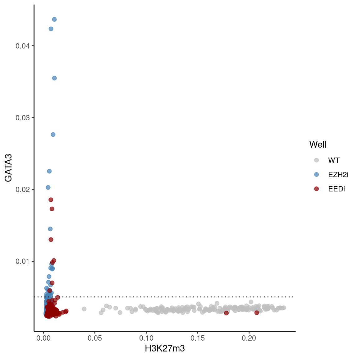

GATA3 vs NANOG per nucleus

ggplot(df, aes(x = NANOG, y = GATA3, color = Well)) + 
  geom_point(alpha = 0.7, size = 2) + 
  scale_color_manual(values = c("grey", "#4682B4", "#8B0000")) + 
  geom_hline(yintercept =cutoff, linetype = "dotted")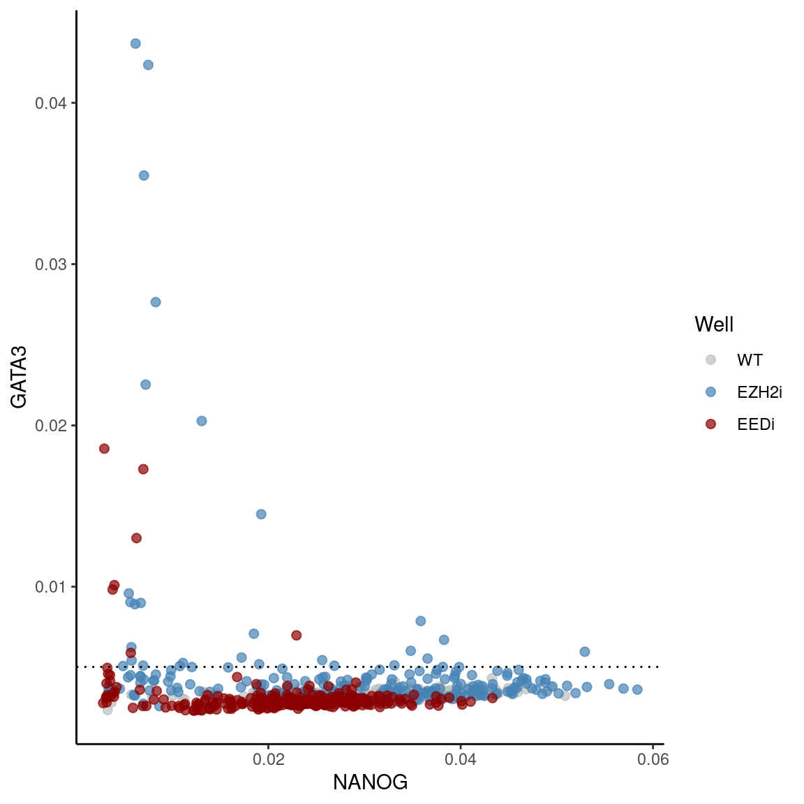

# Total number of cells
perc_positive <- right_join(df %>% group_by(Well) %>% summarise(n_total = n()),
                            df %>% group_by(Well) %>% filter(GATA3 > cutoff) %>% 
                              summarise(n_positive = n()), by="Well") %>%
  mutate(perc_positive = (n_positive / n_total)*100)

perc_positive

# A tibble: 2 × 4
  Well  n_total n_positive perc_positive
  <fct>   <int>      <int>         <dbl>
1 EZH2i     235         28         11.9 
2 EEDi      270          7          2.59

H3K27m3 Timecourse

Channels:

• c1: NANOG
• c2: H3K37m3
• c3: OCT3/4
• c4: DAPI

Metadata_Well:

• A05: Wildtype
• B05: EZH2i_d2
• C05: EZH2i_d4
• D05: EZH2i_d7

expr <- read.table(file.path(params$datadir, "./Timecourse_Well5Nuclei.txt") ,header = TRUE)

expr$Metadata_Well <- factor(
    expr$Metadata_Well,
    levels = c("A05", "B05", "C05", "D05"),
    labels = c("WT", "EZH2i_D2", "EZH2i_D4", "EZH2i_D7")
  )

df <-
  expr %>% dplyr::select(
    Metadata_Well,
    ObjectNumber,
    Metadata_Site,
    Intensity_MeanIntensity_c1_raw,
    Intensity_MeanIntensity_c2_raw,
    Intensity_MeanIntensity_c3_raw,
    Intensity_MeanIntensity_c4_raw
  ) %>%
  rename(
    NANOG = Intensity_MeanIntensity_c1_raw,
    H3K27m3 = Intensity_MeanIntensity_c2_raw,
    OCT = Intensity_MeanIntensity_c3_raw,
    DAPI = Intensity_MeanIntensity_c4_raw,
    Well = Metadata_Well,
    Cell = ObjectNumber,
    Site = Metadata_Site
  )

df_long <- df %>% pivot_longer(c(NANOG, H3K27m3, OCT, DAPI),
                               names_to = "channel", values_to = "value")

my_comparisons <- list(c("EZH2i_D2", "WT"), c("EZH2i_D4", "WT"), c("EZH2i_D7", "WT"))

ggplot(df_long %>% filter(channel == "H3K27m3"),
       aes(y=value, x=Well, color = channel)) + 
  geom_boxplot() + 
  stat_compare_means(comparisons = my_comparisons, method = "t.test") +
  labs(title = "Time course - mean H3K27m3 intensity", y = "Mean intensity", x = "") + 
  theme(axis.text.x = element_text(angle = 45, hjust = 1)) + 
  scale_color_manual(values = c("navy"))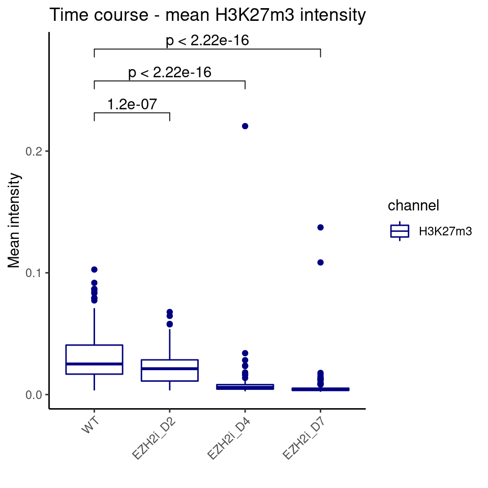

CRISPR/Cas targeting

g1_eed <- read.csv(file.path(params$datadir, "g1_eed.csv"))
g2_eed <- read.csv(file.path(params$datadir, "g2_eed.csv"))

median_1 <- median(g1_eed[g1_eed$Well == "WT", "EED"])
median_2 <- median(g2_eed[g2_eed$Well == "NTgRNA", "EED"])

median_1_gata3 <- median(g1_eed[g1_eed$Well == "WT", "GATA3"])
median_2_gata3 <- median(g2_eed[g2_eed$Well == "NTgRNA", "GATA3"])

merged_rounds <- 
  rbind(g1_eed %>% mutate(round = "1", EED_norm = EED / median_1, GATA3_norm = GATA3 / median_1_gata3), 
        g2_eed %>% mutate(round = "2", EED_norm = EED / median_2, GATA3_norm = GATA3 / median_2_gata3) %>% 
  dplyr::select(!contains("GATA6")))

library(ggrastr)
merged_rounds <- merged_rounds %>% mutate(condition = ifelse(Well == "Transfected", "Transfected", "Control"))

summaries <- merged_rounds %>% 
  group_by(condition) %>% summarise(cutoff = mean(GATA3_norm)*1.5)

cutoff <- summaries[summaries$condition == "Control", "cutoff"][[1]]

# Total number of cells
perc_positive <- right_join(
  merged_rounds %>% group_by(condition, round) %>% summarise(n_total = n()),
  merged_rounds %>% group_by(condition, round) %>% filter(GATA3_norm > cutoff) %>%
    summarise(n_positive = n())) %>%
  mutate(perc_positive = (n_positive / n_total)*100)

perc_positive

# A tibble: 4 × 5
# Groups:   condition [2]
  condition   round n_total n_positive perc_positive
  <chr>       <chr>   <int>      <int>         <dbl>
1 Control     1         853         12          1.41
2 Control     2        1369         19          1.39
3 Transfected 1         958         65          6.78
4 Transfected 2        1132        284         25.1 

ggplot(merged_rounds, 
       aes(x = EED_norm, y = GATA3_norm, color = interaction(Well, round))) + 
  rasterise(geom_point(size = 0.7, alpha = 0.5), dpi = 300) + 
  scale_color_manual(values = c("#f58e8e", "grey", "#99AABB", "#CD5C5C")) +
  labs(title = "Normalized mean intensity across rounds") +
  theme(legend.title = element_blank()) + geom_hline(yintercept = cutoff, linetype = "dotted")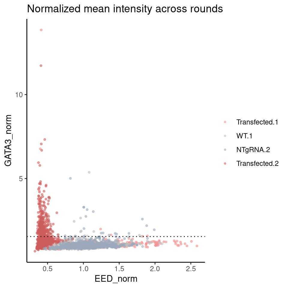

mr_long <- merged_rounds %>% select(Well, Site, round, EED_norm, GATA3_norm) %>% pivot_longer(c(EED_norm, GATA3_norm), names_to = "channel", values_to = "norm_intensity") %>% mutate(condition = ifelse(Well == "Transfected", "Transfected", "Control"))

my_comp <- list(c("Transfected", "Control"))
mr_long$Site <- as.factor(mr_long$Site)
ggplot(mr_long %>% filter(channel == "GATA3_norm"), aes(x=Site, y=norm_intensity, color = condition)) + 
  geom_boxplot() + facet_wrap(round ~ condition)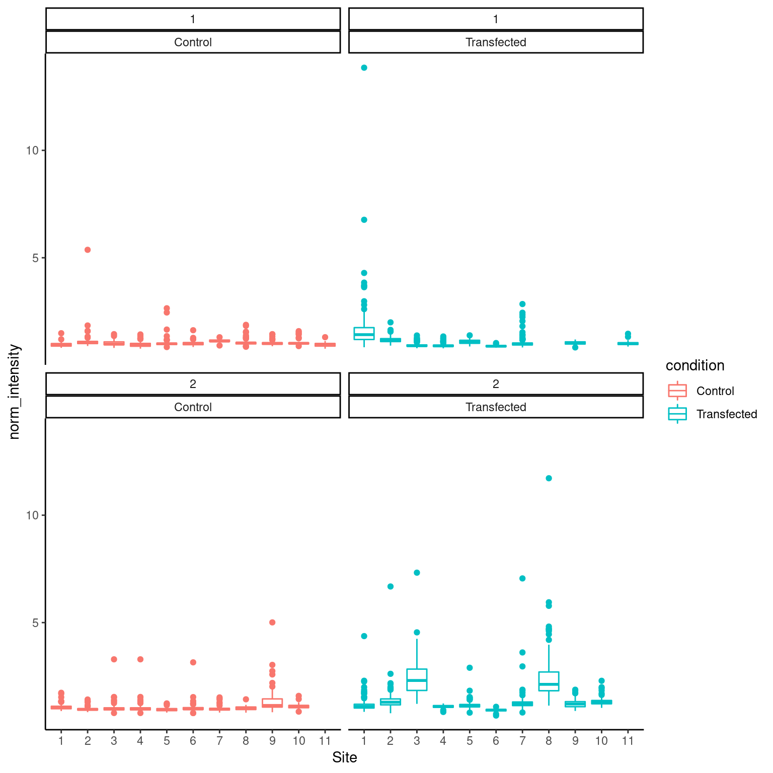

Extended 10a. HS975

old <- theme_set(theme_classic())

expr <- read.table(file.path(params$datadir, "HS975_20xNuclei.txt"), header = TRUE)
expr$Metadata_Site <- sapply(expr$Metadata_Site, as.factor)

# Rename wells for readability
expr$Metadata_Well <- factor(expr$Metadata_Well, levels = c("A01", "B01"),
                             labels = c("WT", "EZH2i"))
well <- filter(expr, expr$Intensity_MeanIntensity_c4_raw >= 0.025)

df <-
  well %>% select(
    Metadata_Well,
    ObjectNumber,
    Metadata_Site,
    Intensity_MeanIntensity_c1_raw,
    Intensity_MeanIntensity_c2_raw,
    Intensity_MeanIntensity_c3_raw,
    Intensity_MeanIntensity_c4_raw
  ) %>%
  rename(
    GATA6 = Intensity_MeanIntensity_c1_raw,
    H3K27m3 = Intensity_MeanIntensity_c2_raw,
    GATA3 = Intensity_MeanIntensity_c3_raw,
    DAPI = Intensity_MeanIntensity_c4_raw,
    Well = Metadata_Well,
    Cell = ObjectNumber,
    Site = Metadata_Site
  )

noise_cutoff <- 0.007
df <- df %>% filter(GATA3 > noise_cutoff)

summaries <- df %>% 
  group_by(Well) %>% summarise(cutoff = mean(GATA3)*1.5)
cutoff <- summaries[summaries$Well == "WT", "cutoff"][[1]]
perc_positive <- right_join(df %>% group_by(Well) %>% summarise(n_total = n()),
                            df %>% group_by(Well) %>% filter(GATA3 > cutoff) %>%
                              summarise(n_positive = n())) %>%
  mutate(perc_positive = (n_positive / n_total)*100)

perc_positive

# A tibble: 1 × 4
  Well  n_total n_positive perc_positive
  <fct>   <int>      <int>         <dbl>
1 EZH2i     127          8          6.30

df_long <- df %>% pivot_longer(!c(Well, Cell, Site),
                               names_to = "channel", values_to = "value")

ggplot(df_long %>% filter(channel %in% c("GATA3", "H3K27m3")), aes(y=value, x=Well, color=Well)) + 
  geom_boxplot() + facet_grid(. ~ channel, scales = "free_y") + 
  stat_compare_means(method="t.test")

Session information

sessionInfo()

R version 4.1.2 (2021-11-01)
Platform: x86_64-pc-linux-gnu (64-bit)
Running under: Ubuntu 20.04.3 LTS

Matrix products: default
BLAS:   /usr/lib/x86_64-linux-gnu/openblas-pthread/libblas.so.3
LAPACK: /usr/lib/x86_64-linux-gnu/openblas-pthread/liblapack.so.3

locale:
 [1] LC_CTYPE=en_US.UTF-8       LC_NUMERIC=C              
 [3] LC_TIME=sv_SE.UTF-8        LC_COLLATE=en_US.UTF-8    
 [5] LC_MONETARY=sv_SE.UTF-8    LC_MESSAGES=en_US.UTF-8   
 [7] LC_PAPER=sv_SE.UTF-8       LC_NAME=C                 
 [9] LC_ADDRESS=C               LC_TELEPHONE=C            
[11] LC_MEASUREMENT=sv_SE.UTF-8 LC_IDENTIFICATION=C       

attached base packages:
[1] stats4    stats     graphics  grDevices utils     datasets  methods  
[8] base     

other attached packages:
 [1] svglite_2.0.0               heatmaply_1.3.0            
 [3] viridis_0.6.2               viridisLite_0.4.0          
 [5] plotly_4.10.0               gtools_3.9.2               
 [7] ggpubr_0.4.0                readxl_1.3.1               
 [9] wigglescout_0.13.5          cowplot_1.1.1              
[11] DESeq2_1.34.0               SummarizedExperiment_1.24.0
[13] Biobase_2.54.0              MatrixGenerics_1.6.0       
[15] matrixStats_0.61.0          ggrastr_0.2.3              
[17] forcats_0.5.1               stringr_1.4.0              
[19] dplyr_1.0.7                 purrr_0.3.4                
[21] readr_2.1.0                 tidyr_1.1.4                
[23] tibble_3.1.6                ggplot2_3.3.5              
[25] tidyverse_1.3.1             rtracklayer_1.54.0         
[27] GenomicRanges_1.46.0        GenomeInfoDb_1.30.0        
[29] IRanges_2.28.0              S4Vectors_0.32.2           
[31] BiocGenerics_0.40.0         workflowr_1.6.2            

loaded via a namespace (and not attached):
  [1] backports_1.3.0          systemfonts_1.0.3        plyr_1.8.6              
  [4] lazyeval_0.2.2           splines_4.1.2            crosstalk_1.2.0         
  [7] BiocParallel_1.28.0      listenv_0.8.0            digest_0.6.28           
 [10] foreach_1.5.1            htmltools_0.5.2          fansi_0.5.0             
 [13] magrittr_2.0.1           memoise_2.0.0            tzdb_0.2.0              
 [16] globals_0.14.0           Biostrings_2.62.0        annotate_1.72.0         
 [19] modelr_0.1.8             colorspace_2.0-2         blob_1.2.2              
 [22] rvest_1.0.2              haven_2.4.3              xfun_0.28               
 [25] crayon_1.4.2             RCurl_1.98-1.5           jsonlite_1.7.2          
 [28] genefilter_1.76.0        iterators_1.0.13         survival_3.2-13         
 [31] glue_1.5.1               registry_0.5-1           gtable_0.3.0            
 [34] zlibbioc_1.40.0          XVector_0.34.0           webshot_0.5.2           
 [37] DelayedArray_0.20.0      car_3.0-12               abind_1.4-5             
 [40] scales_1.1.1             DBI_1.1.1                rstatix_0.7.0           
 [43] Rcpp_1.0.7               xtable_1.8-4             bit_4.0.4               
 [46] htmlwidgets_1.5.4        httr_1.4.2               RColorBrewer_1.1-2      
 [49] ellipsis_0.3.2           farver_2.1.0             pkgconfig_2.0.3         
 [52] XML_3.99-0.8             sass_0.4.0               dbplyr_2.1.1            
 [55] locfit_1.5-9.4           utf8_1.2.2               labeling_0.4.2          
 [58] tidyselect_1.1.1         rlang_0.4.12             reshape2_1.4.4          
 [61] later_1.3.0              AnnotationDbi_1.56.2     munsell_0.5.0           
 [64] cellranger_1.1.0         tools_4.1.2              cachem_1.0.6            
 [67] cli_3.1.0                generics_0.1.1           RSQLite_2.2.8           
 [70] broom_0.7.10             evaluate_0.14            fastmap_1.1.0           
 [73] yaml_2.2.1               knitr_1.36               bit64_4.0.5             
 [76] fs_1.5.0                 dendextend_1.15.2        KEGGREST_1.34.0         
 [79] future_1.23.0            whisker_0.4              xml2_1.3.2              
 [82] compiler_4.1.2           rstudioapi_0.13          beeswarm_0.4.0          
 [85] png_0.1-7                ggsignif_0.6.3           reprex_2.0.1            
 [88] geneplotter_1.72.0       bslib_0.3.1              stringi_1.7.6           
 [91] highr_0.9                lattice_0.20-45          Matrix_1.4-0            
 [94] vctrs_0.3.8              pillar_1.6.4             lifecycle_1.0.1         
 [97] furrr_0.2.3              jquerylib_0.1.4          data.table_1.14.2       
[100] bitops_1.0-7             seriation_1.3.1          httpuv_1.6.3            
[103] R6_2.5.1                 BiocIO_1.4.0             TSP_1.1-11              
[106] promises_1.2.0.1         gridExtra_2.3            vipor_0.4.5             
[109] parallelly_1.28.1        codetools_0.2-18         assertthat_0.2.1        
[112] rprojroot_2.0.2          rjson_0.2.20             withr_2.4.2             
[115] GenomicAlignments_1.30.0 Rsamtools_2.10.0         GenomeInfoDbData_1.2.7  
[118] parallel_4.1.2           hms_1.1.1                grid_4.1.2              
[121] rmarkdown_2.11           carData_3.0-4            Cairo_1.5-12.2          
[124] git2r_0.28.0             lubridate_1.8.0          ggbeeswarm_0.6.0        
[127] restfulr_0.0.13