Histone marks on bivalent chromatin
Carmen Navarro
2021-02-03
Last updated: 2021-02-03
Checks: 7 0
Knit directory: hesc-epigenomics/
This reproducible R Markdown analysis was created with workflowr (version 1.6.2). The Checks tab describes the reproducibility checks that were applied when the results were created. The Past versions tab lists the development history.
Great! Since the R Markdown file has been committed to the Git repository, you know the exact version of the code that produced these results.
Great job! The global environment was empty. Objects defined in the global environment can affect the analysis in your R Markdown file in unknown ways. For reproduciblity it’s best to always run the code in an empty environment.
The command set.seed(20210202) was run prior to running the code in the R Markdown file. Setting a seed ensures that any results that rely on randomness, e.g. subsampling or permutations, are reproducible.
Great job! Recording the operating system, R version, and package versions is critical for reproducibility.
Nice! There were no cached chunks for this analysis, so you can be confident that you successfully produced the results during this run.
Great job! Using relative paths to the files within your workflowr project makes it easier to run your code on other machines.
Great! You are using Git for version control. Tracking code development and connecting the code version to the results is critical for reproducibility.
The results in this page were generated with repository version 70a54dd. See the Past versions tab to see a history of the changes made to the R Markdown and HTML files.
Note that you need to be careful to ensure that all relevant files for the analysis have been committed to Git prior to generating the results (you can use wflow_publish or wflow_git_commit). workflowr only checks the R Markdown file, but you know if there are other scripts or data files that it depends on. Below is the status of the Git repository when the results were generated:
Ignored files:
    Ignored:    .Rproj.user/
    Ignored:    data/bed/
    Ignored:    data/bw
    Ignored:    data/meta/
    Ignored:    data/peaks

Unstaged changes:
    Modified:   .gitignore
Note that any generated files, e.g. HTML, png, CSS, etc., are not included in this status report because it is ok for generated content to have uncommitted changes.
These are the previous versions of the repository in which changes were made to the R Markdown (analysis/bivalent_chromatin.Rmd) and HTML (docs/bivalent_chromatin.html) files. If you’ve configured a remote Git repository (see ?wflow_git_remote), click on the hyperlinks in the table below to view the files as they were in that past version.
| File | Version | Author | Date | Message |
|---|---|---|---|---|
| Rmd | 70a54dd | cnluzon | 2021-02-03 | Bivalent chromatin profiles |
Summary
This is a study on bivalent chromatin regions.
As a base annotation we use the bivalent regions annotated in Court 2017:
Court, Franck, and Philippe Arnaud. “An annotated list of bivalent chromatin regions in human ES cells: a new tool for cancer epigenetic research.” Oncotarget 8.3 (2017): 4110.
Additionally, the bivalent genes annotated as such in their supplementary file 1: https://www.oncotarget.com/index.php?journal=oncotarget&page=article&op=downloadSuppFile&path%5B%5D=13746&path%5B%5D=21048
Bivalent regions file: Original regions were translated to hg38 with liftOver: data/bed/Bivalent_Court2017.hg38.bed.
colors_list <- c("Naive_EZH2i"="#5F9EA0",
                 "Naive_Untreated"="#278b8b",
                 "Primed_EZH2i"="#f47770",
                 "Primed_Untreated"="#f44b34")

style_info <- read.table(params$styles, header = T, sep = "\t")
rownames(style_info) <- style_info$bw
Bivalent regions
biv_ranges <- import(params$biv, )
biv_ranges
GRanges object with 5763 ranges and 0 metadata columns:
seqnames ranges strand
<Rle> <IRanges> <Rle>
[1] chr1 922893-927228 *
[2] chr1 938978-943553 *
[3] chr1 958524-962043 *
[4] chr1 965864-967597 *
[5] chr1 997897-1002325 *
... ... ... ...
[5759] chr22 50269325-50272471 *
[5760] chr22 50305876-50307401 *
[5761] chr22 50529375-50532912 *
[5762] chr22 50672502-50674162 *
[5763] chr22 50696573-50698241 *
-------
seqinfo: 22 sequences from an unspecified genome; no seqlengthsH3K4m3
bwfiles <- list.files(file.path(params$datadir, "bw/Kumar_2020/hu2"), full.names = T)

bwinput <- bwfiles[grepl("IN.*pooled", bwfiles)]
bwfiles <- bwfiles[grepl("H3K4m3.*pooled.hg38.scaled", bwfiles)]

colors <- as.character(style_info[basename(c(bwfiles, bwinput)), "color_cond"])
labels <- style_info[basename(c(bwfiles, bwinput)), "label"]

plot_bw_profile(
  c(bwfiles, bwinput),
  params$biv,
  mode = "center",
  upstream = 10000,
  downstream = 10000,
  colors = colors,
  labels = labels
) + ggtitle("H3K4m3 at bivalent regions")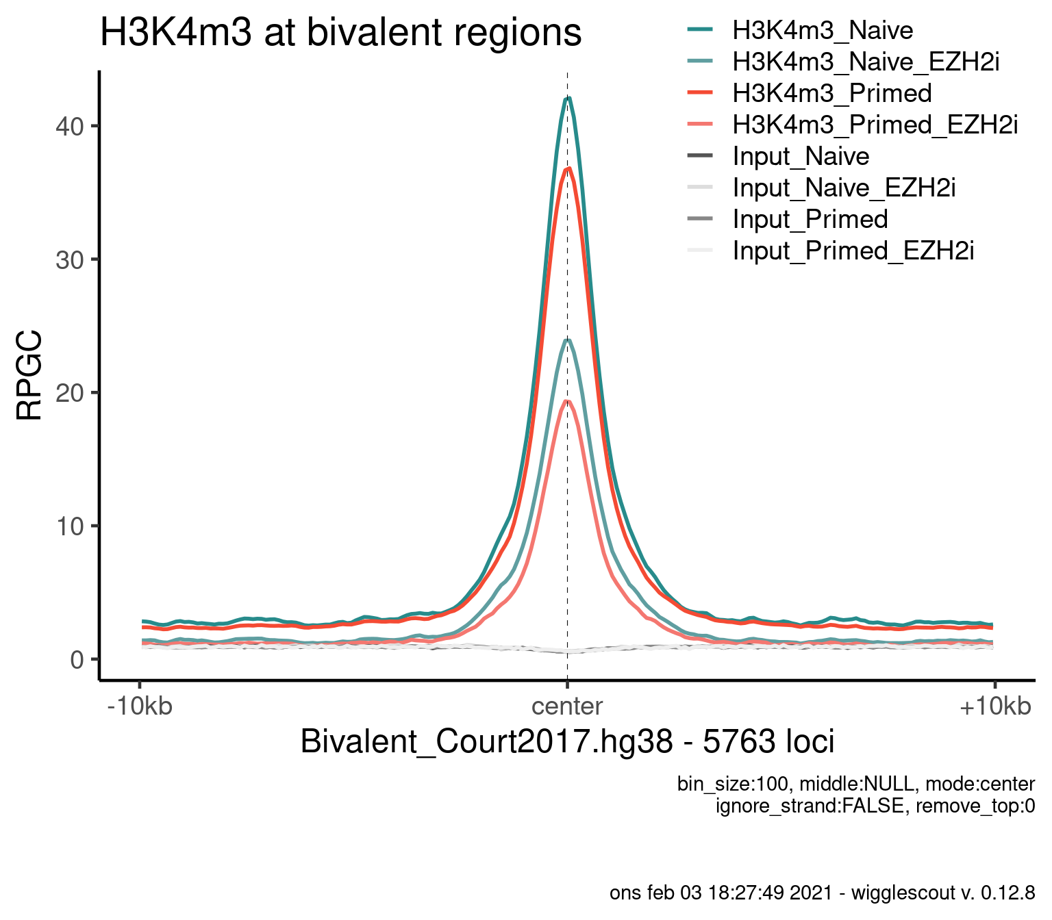
Norm to input:
bwfiles <- list.files(file.path(params$datadir, "bw/Kumar_2020/hu2"), full.names = T)

bwinput <- bwfiles[grepl("IN.*pooled", bwfiles)]
bwfiles <- bwfiles[grepl("H3K4m3.*pooled.hg38.scaled", bwfiles)]

colors <- as.character(style_info[basename(bwfiles), "color_cond"])
labels <- style_info[basename(bwfiles), "label"]

plot_bw_profile(
  bwfiles,
  bg_bwfiles = bwinput,
  params$biv,
  mode = "center",
  upstream = 10000,
  downstream = 10000,
  colors = colors,
  labels = labels
) + ggtitle("H3K4m3 at bivalent regions")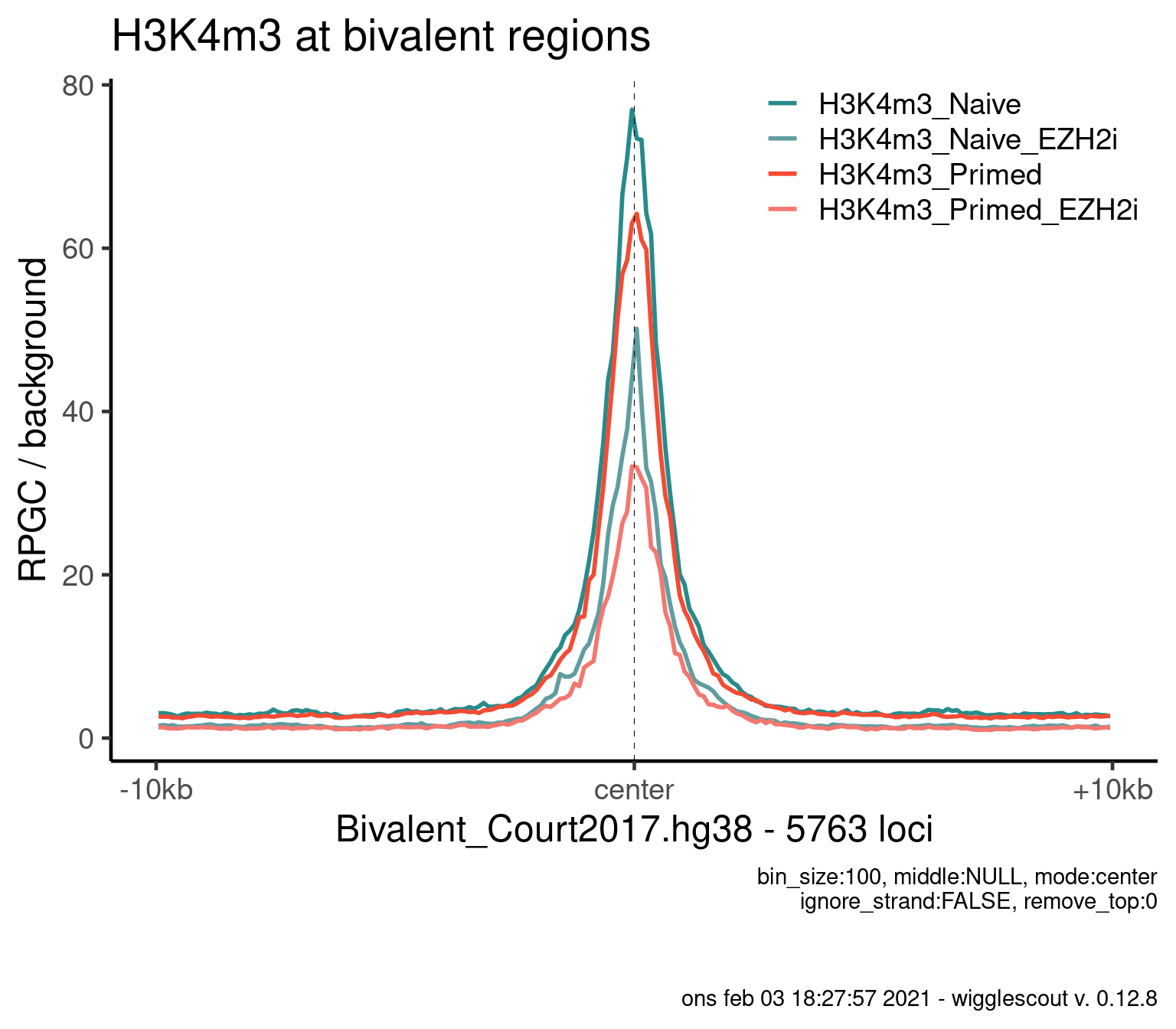
H3K27m3
bwfiles <- list.files(file.path(params$datadir, "bw/Kumar_2020/hu2"), full.names = T)

bwinput <- bwfiles[grepl("IN.*pooled", bwfiles)]
bwfiles <- bwfiles[grepl("H3K27m3.*pooled.hg38.scaled", bwfiles)]

colors <- as.character(style_info[basename(c(bwfiles, bwinput)), "color_cond"])
labels <- style_info[basename(c(bwfiles, bwinput)), "label"]

plot_bw_profile(
  c(bwfiles, bwinput),
  params$biv,
  mode = "center",
  upstream = 10000,
  downstream = 10000,
  colors = colors,
  labels = labels
) + ggtitle("H3K27m3 at bivalent regions")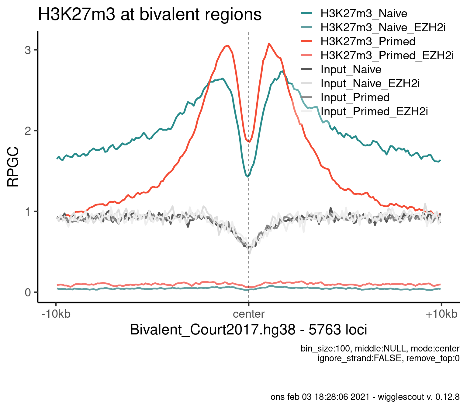
Norm to input:
bwfiles <- list.files(file.path(params$datadir, "bw/Kumar_2020/hu2"), full.names = T)

bwinput <- bwfiles[grepl("IN.*pooled", bwfiles)]
bwfiles <- bwfiles[grepl("H3K27m3.*pooled.hg38.scaled", bwfiles)]

colors <- as.character(style_info[basename(bwfiles), "color_cond"])
labels <- style_info[basename(bwfiles), "label"]

plot_bw_profile(
  bwfiles,
  bg_bwfiles = bwinput,
  params$biv,
  mode = "center",
  upstream = 10000,
  downstream = 10000,
  colors = colors,
  labels = labels,
  bin_size = 200
) + ggtitle("H3K27m3 at bivalent regions")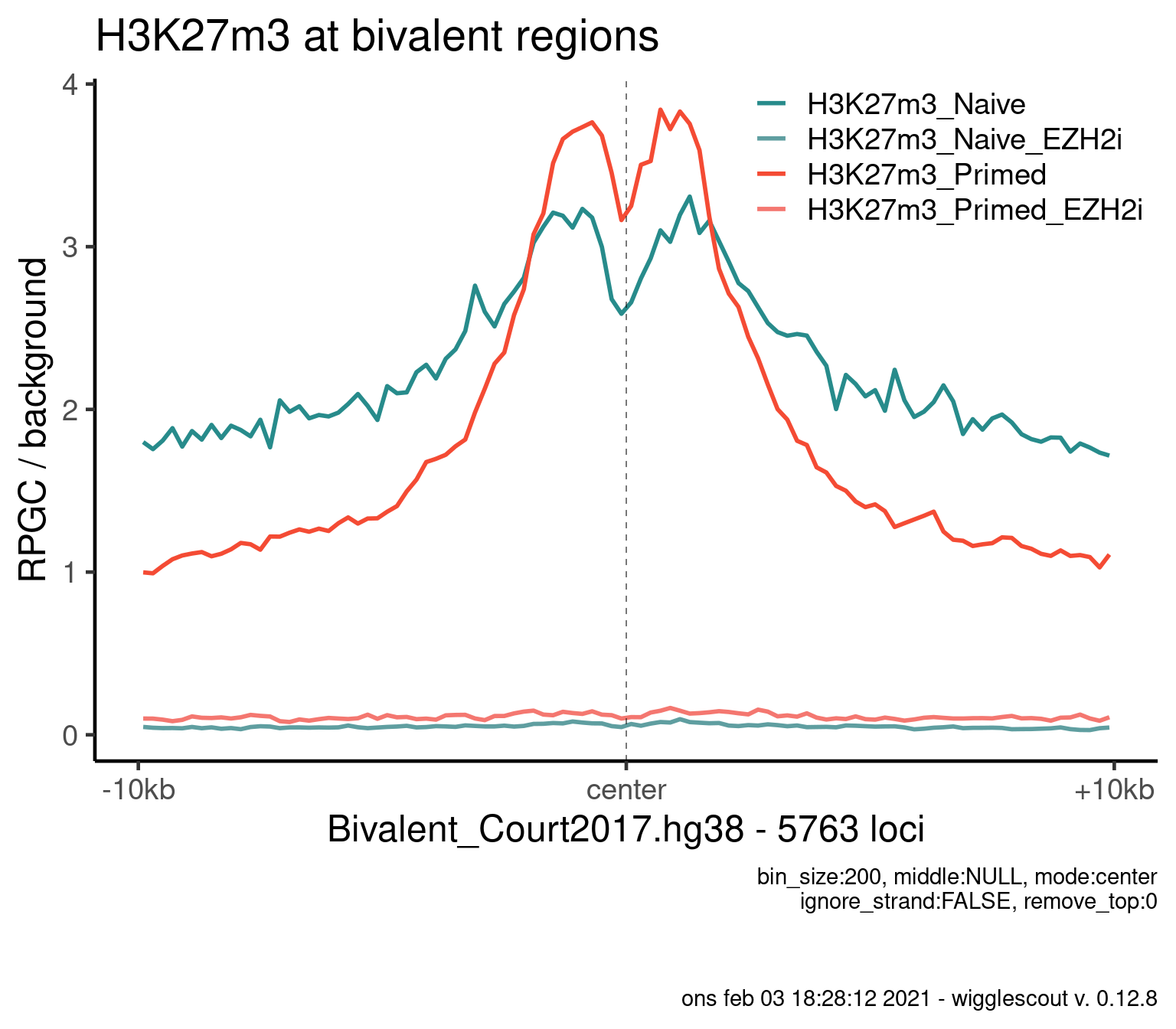
H2AUb
bwfiles <- list.files(file.path(params$datadir, "bw/Kumar_2020/hu2"), full.names = T)

bwinput <- bwfiles[grepl("IN.*pooled", bwfiles)]
bwfiles <- bwfiles[grepl("H2A.*pooled.hg38.scaled", bwfiles)]

colors <- as.character(style_info[basename(c(bwfiles, bwinput)), "color_cond"])
labels <- style_info[basename(c(bwfiles, bwinput)), "label"]

plot_bw_profile(
  c(bwfiles, bwinput),
  params$biv,
  mode = "center",
  upstream = 10000,
  downstream = 10000,
  colors = colors,
  labels = labels
) + ggtitle("H2Aub at bivalent regions")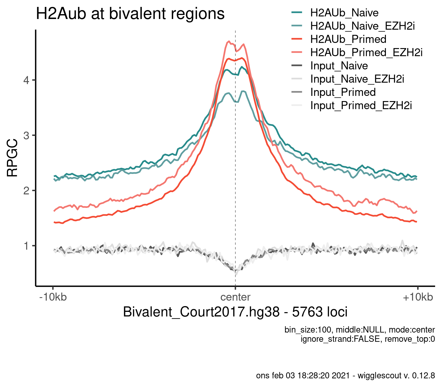
Norm to input:
bwfiles <- list.files(file.path(params$datadir, "bw/Kumar_2020/hu2"), full.names = T)

bwinput <- bwfiles[grepl("IN.*pooled", bwfiles)]
bwfiles <- bwfiles[grepl("H2A.*pooled.hg38.scaled", bwfiles)]

colors <- as.character(style_info[basename(bwfiles), "color_cond"])
labels <- style_info[basename(bwfiles), "label"]

plot_bw_profile(
  bwfiles,
  bg_bwfiles = bwinput,
  params$biv,
  mode = "center",
  upstream = 10000,
  downstream = 10000,
  colors = colors,
  labels = labels,
  bin_size = 200
) + ggtitle("H2Aub at bivalent regions")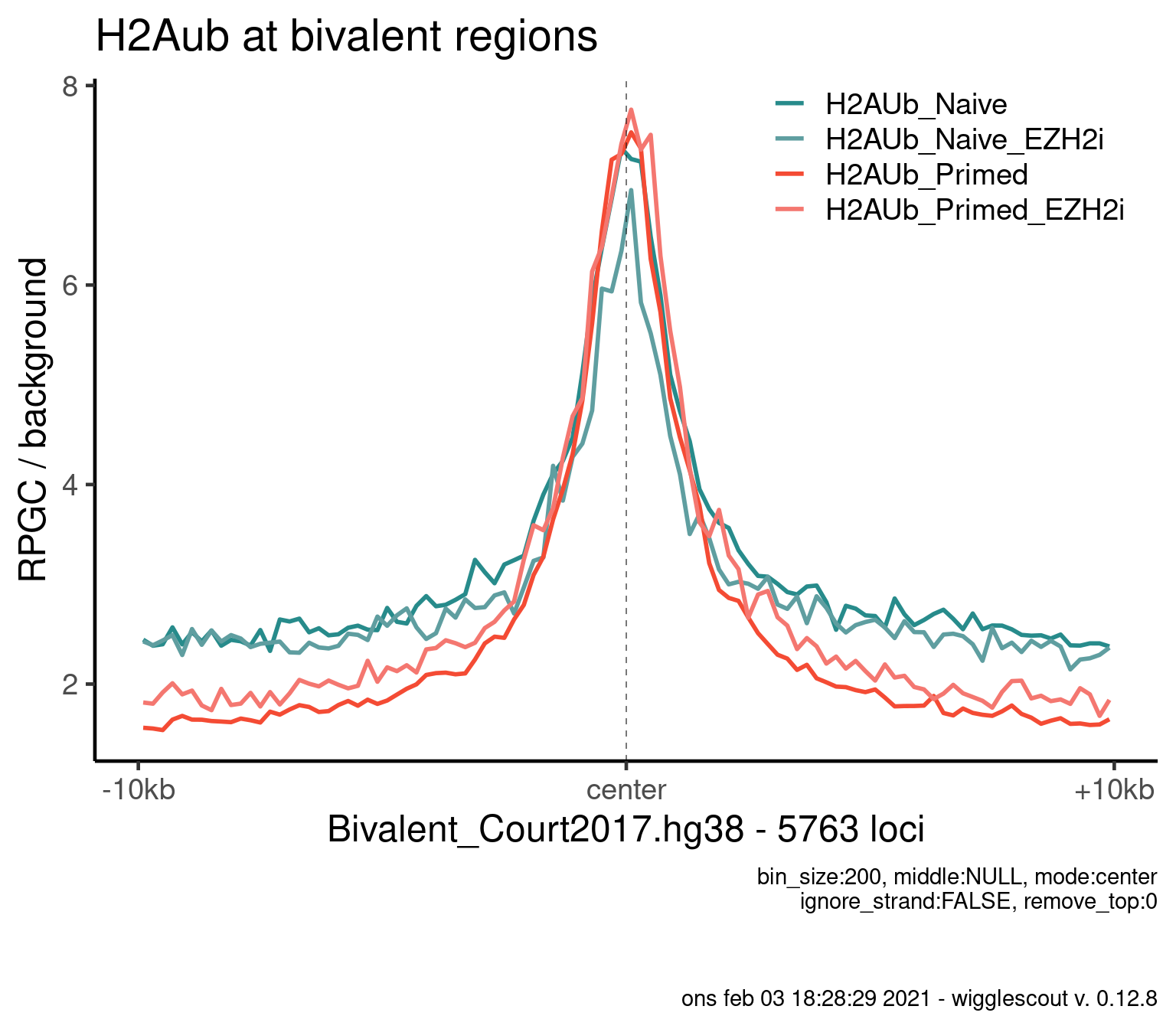
sessionInfo()R version 4.0.3 (2020-10-10)
Platform: x86_64-pc-linux-gnu (64-bit)
Running under: Ubuntu 20.04.1 LTS
Matrix products: default
BLAS: /usr/lib/x86_64-linux-gnu/openblas-pthread/libblas.so.3
LAPACK: /usr/lib/x86_64-linux-gnu/openblas-pthread/liblapack.so.3
locale:
[1] LC_CTYPE=en_US.UTF-8 LC_NUMERIC=C
[3] LC_TIME=sv_SE.UTF-8 LC_COLLATE=en_US.UTF-8
[5] LC_MONETARY=sv_SE.UTF-8 LC_MESSAGES=en_US.UTF-8
[7] LC_PAPER=sv_SE.UTF-8 LC_NAME=C
[9] LC_ADDRESS=C LC_TELEPHONE=C
[11] LC_MEASUREMENT=sv_SE.UTF-8 LC_IDENTIFICATION=C
attached base packages:
[1] stats4 parallel stats graphics grDevices utils datasets
[8] methods base
other attached packages:
[1] purrr_0.3.4
[2] ggplot2_3.3.3
[3] rtracklayer_1.50.0
[4] org.Hs.eg.db_3.11.4
[5] TxDb.Hsapiens.UCSC.hg38.knownGene_3.10.0
[6] GenomicFeatures_1.40.1
[7] AnnotationDbi_1.52.0
[8] Biobase_2.50.0
[9] GenomicRanges_1.42.0
[10] GenomeInfoDb_1.26.2
[11] IRanges_2.24.1
[12] S4Vectors_0.28.1
[13] BiocGenerics_0.36.0
[14] wigglescout_0.12.8
[15] workflowr_1.6.2
loaded via a namespace (and not attached):
[1] bitops_1.0-6 matrixStats_0.57.0
[3] fs_1.5.0 bit64_4.0.5
[5] RColorBrewer_1.1-2 progress_1.2.2
[7] httr_1.4.2 rprojroot_2.0.2
[9] tools_4.0.3 R6_2.5.0
[11] DBI_1.1.0 colorspace_2.0-0
[13] withr_2.4.0 tidyselect_1.1.0
[15] prettyunits_1.1.1 curl_4.3
[17] bit_4.0.4 compiler_4.0.3
[19] git2r_0.27.1 xml2_1.3.2
[21] DelayedArray_0.16.0 labeling_0.4.2
[23] scales_1.1.1 askpass_1.1
[25] rappdirs_0.3.1 stringr_1.4.0
[27] digest_0.6.27 Rsamtools_2.6.0
[29] rmarkdown_2.6 XVector_0.30.0
[31] pkgconfig_2.0.3 htmltools_0.5.1
[33] parallelly_1.23.0 MatrixGenerics_1.2.0
[35] dbplyr_2.0.0 rlang_0.4.10
[37] rstudioapi_0.13 RSQLite_2.2.1
[39] farver_2.0.3 generics_0.1.0
[41] BiocParallel_1.24.1 dplyr_1.0.3
[43] RCurl_1.98-1.2 magrittr_2.0.1
[45] GenomeInfoDbData_1.2.4 Matrix_1.3-2
[47] Rcpp_1.0.6 munsell_0.5.0
[49] lifecycle_0.2.0 furrr_0.2.1
[51] stringi_1.5.3 whisker_0.4
[53] yaml_2.2.1 SummarizedExperiment_1.20.0
[55] zlibbioc_1.36.0 plyr_1.8.6
[57] BiocFileCache_1.12.1 grid_4.0.3
[59] blob_1.2.1 listenv_0.8.0
[61] promises_1.1.1 crayon_1.3.4
[63] lattice_0.20-41 Biostrings_2.58.0
[65] hms_0.5.3 knitr_1.30
[67] pillar_1.4.7 reshape2_1.4.4
[69] codetools_0.2-18 biomaRt_2.44.4
[71] XML_3.99-0.5 glue_1.4.2
[73] evaluate_0.14 vctrs_0.3.6
[75] httpuv_1.5.4 gtable_0.3.0
[77] openssl_1.4.3 future_1.21.0
[79] assertthat_0.2.1 xfun_0.20
[81] later_1.1.0.1 tibble_3.0.5
[83] GenomicAlignments_1.26.0 memoise_1.1.0
[85] globals_0.14.0 ellipsis_0.3.1