Figure 1. Global histone levels.
Carmen Navarro
Updated: 2021-07-01
Last updated: 2021-07-01
Checks: 7 0
Knit directory: hesc-epigenomics/
This reproducible R Markdown analysis was created with workflowr (version 1.6.2). The Checks tab describes the reproducibility checks that were applied when the results were created. The Past versions tab lists the development history.
Great! Since the R Markdown file has been committed to the Git repository, you know the exact version of the code that produced these results.
Great job! The global environment was empty. Objects defined in the global environment can affect the analysis in your R Markdown file in unknown ways. For reproduciblity it’s best to always run the code in an empty environment.
The command set.seed(20210202) was run prior to running the code in the R Markdown file. Setting a seed ensures that any results that rely on randomness, e.g. subsampling or permutations, are reproducible.
Great job! Recording the operating system, R version, and package versions is critical for reproducibility.
Nice! There were no cached chunks for this analysis, so you can be confident that you successfully produced the results during this run.
Great job! Using relative paths to the files within your workflowr project makes it easier to run your code on other machines.
Great! You are using Git for version control. Tracking code development and connecting the code version to the results is critical for reproducibility.
The results in this page were generated with repository version 5976105. See the Past versions tab to see a history of the changes made to the R Markdown and HTML files.
Note that you need to be careful to ensure that all relevant files for the analysis have been committed to Git prior to generating the results (you can use wflow_publish or wflow_git_commit). workflowr only checks the R Markdown file, but you know if there are other scripts or data files that it depends on. Below is the status of the Git repository when the results were generated:
Ignored files:
    Ignored:    .Rhistory
    Ignored:    .Rproj.user/
    Ignored:    analysis/figure/
    Ignored:    data/bed/
    Ignored:    data/bw
    Ignored:    data/igv/
    Ignored:    data/liftover/
    Ignored:    data/other/
    Ignored:    data/peaks
    Ignored:    data/rnaseq/

Untracked files:
    Untracked:  data/meta/Kumar_2020_bins_panels_design.csv
    Untracked:  data/meta/Kumar_2020_master_bins_10kb_table_raw.tsv
    Untracked:  data/meta/Kumar_2020_master_bins_5kb_table_raw.tsv
    Untracked:  data/meta/Kumar_2020_master_bins_5kb_table_raw.zip
    Untracked:  data/meta/Kumar_2020_master_bins_5kb_table_replicates_only.tsv
    Untracked:  data/meta/Kumar_2020_master_bins_5kb_table_shrunk.tsv
    Untracked:  data/meta/Kumar_2020_master_bins_5kb_table_shrunk.zip
    Untracked:  data/meta/Kumar_2020_master_gene_table.zip
    Untracked:  data/meta/Kumar_2020_master_gene_table_rnaseq_shrunk.tsv
    Untracked:  data/meta/Kumar_2020_master_gene_table_rnaseq_shrunk_plus_annotations.tsv
    Untracked:  data/meta/Kumar_2020_master_gene_table_rnaseq_shrunk_plus_annotations.zip
    Untracked:  data/meta/Kumar_2020_promoters_panels_design.csv
    Untracked:  data/meta/gene_names_bivalent.tsv
Note that any generated files, e.g. HTML, png, CSS, etc., are not included in this status report because it is ok for generated content to have uncommitted changes.
These are the previous versions of the repository in which changes were made to the R Markdown (analysis/fig_01_quantitative_chip.Rmd) and HTML (docs/fig_01_quantitative_chip.html) files. If you’ve configured a remote Git repository (see ?wflow_git_remote), click on the hyperlinks in the table below to view the files as they were in that past version.
| File | Version | Author | Date | Message |
|---|---|---|---|---|
| Rmd | 5976105 | C. Navarro | 2021-07-01 | wflow_publish(“./analysis/fig_01_quantitative_chip.Rmd”, verbose = T) |
| Rmd | 9e8b1a9 | cnluzon | 2021-05-26 | Metadata folder added |
| html | 9e8b1a9 | cnluzon | 2021-05-26 | Metadata folder added |
| html | a9d0a78 | cnluzon | 2021-04-13 | Build site. |
| Rmd | dcfe4a4 | cnluzon | 2021-04-13 | wflow_publish(“./analysis/fig_01_quantitative_chip.Rmd”) |
| html | 054d3f5 | cnluzon | 2021-03-22 | Build site. |
| Rmd | 07bb6d9 | cnluzon | 2021-03-22 | H9 ChromHMM annotation |
| html | a6a00b6 | cnluzon | 2021-03-12 | Fig1 with ttest |
| Rmd | 8f01ba6 | cnluzon | 2021-03-12 | Stat tests in global counts |
| Rmd | 0f37941 | cnluzon | 2021-03-12 | Fig1 fresh |
| html | 0f37941 | cnluzon | 2021-03-12 | Fig1 fresh |
Summary
Supplementary code for panel 1 figures.
Helper functions
#' Calculate INRC from a mapped read counts table, and append such values
#' to it.
#'
#' @param counts Counts table. Corresponding file is provided as part of the
#'   included metadata.
#' @param selector Counts column used. Final_mapped represents the final number
#'   of reads after deduplication and blacklisting.

#' @return A table including INRC and INRC norm to naive reference
calculate_inrc <- function(counts, selector = "final_mapped") {
  counts$condition <- paste(counts$celltype, counts$treatment, sep="_")

  inputs <- counts[counts$ip == "Input", c("library", selector)]
  colnames(inputs) <- c("library", "input_reads")

  non_inputs <- counts[counts$ip != "Input",]
  counts <- merge(non_inputs, inputs, by.x="input", by.y="library")
  counts$inrc <- counts[, selector] / counts[, "input_reads"]

  references <- counts[grepl("_Ni_pooled", counts$library), c("ip", "inrc")]
  colnames(references) <- c("ip", "ref_inrc")

  counts <- merge(counts, references, by="ip")
  counts$norm_to_naive <- counts$inrc / counts$ref_inrc

  id_vars <- c("ip", "treatment", "celltype", "condition", "replicate", "norm_to_naive")
  inrc <- counts[, c(id_vars)]

  inrc$condition <- factor(
    inrc$condition,
    levels = c(
      "Naive_Untreated",
      "Primed_Untreated",
      "Naive_EZH2i",
      "Primed_EZH2i"
    )
  )

  inrc
}

#' Barplot INRC pooled vs replicates per condition
#'
#' @param inrc Table with the INRC values
#' @param ip Which IP to plot
#' @param colors Corresponding colors
inrc_barplot <- function(inrc, ip, colors, font = 16) {
  inrc <- inrc[inrc$ip == ip, ]

  # So paired test takes right replicates
  inrc <- inrc[order(inrc$condition, inrc$replicate), ]

  max_v <- max(abs(inrc$norm_to_naive))

  aesthetics <- aes(x = .data[["condition"]],
                    y = .data[["norm_to_naive"]],
                    color = .data[["condition"]])

  my_comp <- list(c("Naive_Untreated", "Primed_Untreated"),
                  c("Naive_Untreated", "Naive_EZH2i"),
                  c("Primed_Untreated", "Primed_EZH2i"),
                  c("Naive_EZH2i", "Primed_EZH2i"))

  stats_method <- "t.test"

  ggplot(inrc[inrc$replicate != 'pooled',], aesthetics) +
    geom_point() +
    stat_compare_means(
      method = stats_method,
      paired = TRUE,
      comparisons = my_comp,
      label = "p.format"
    ) +
    geom_bar(
      data = inrc[inrc$replicate == 'pooled',],
      stat = 'identity',
      alpha = 0.6,
      aes(fill = condition)
    ) +
    scale_fill_manual(values = colors) +
    scale_color_manual(values = colors) +
    labs(
      x = "",
      y = 'INRC fraction vs Naïve',
      title = paste(ip, "MINUTE-ChIP"),
      caption = paste(stats_method, "signif. test, paired")
    ) +
    theme_classic(base_size = font) +
    theme(axis.text.x = element_text(angle = 45, hjust = 1)) +
    ylim(0, 1.5)
}

colors_list <- c("Naive_EZH2i"="#82c5c6",
                 "Naive_Untreated"="#278b8b",
                 "Primed_EZH2i"="#f49797",
                 "Primed_Untreated"="#f44b34")
Global read counts
H2AUb levels
counts_file <- file.path(params$datadir, "meta", "Kumar_2020_stats_summary.csv")
counts <- read.table(counts_file, sep="\t", header = T, na.strings = "NA", stringsAsFactors = F)

inrc <- calculate_inrc(counts)
ip <- "H2Aub"

inrc_barplot(inrc, "H2Aub", colors_list)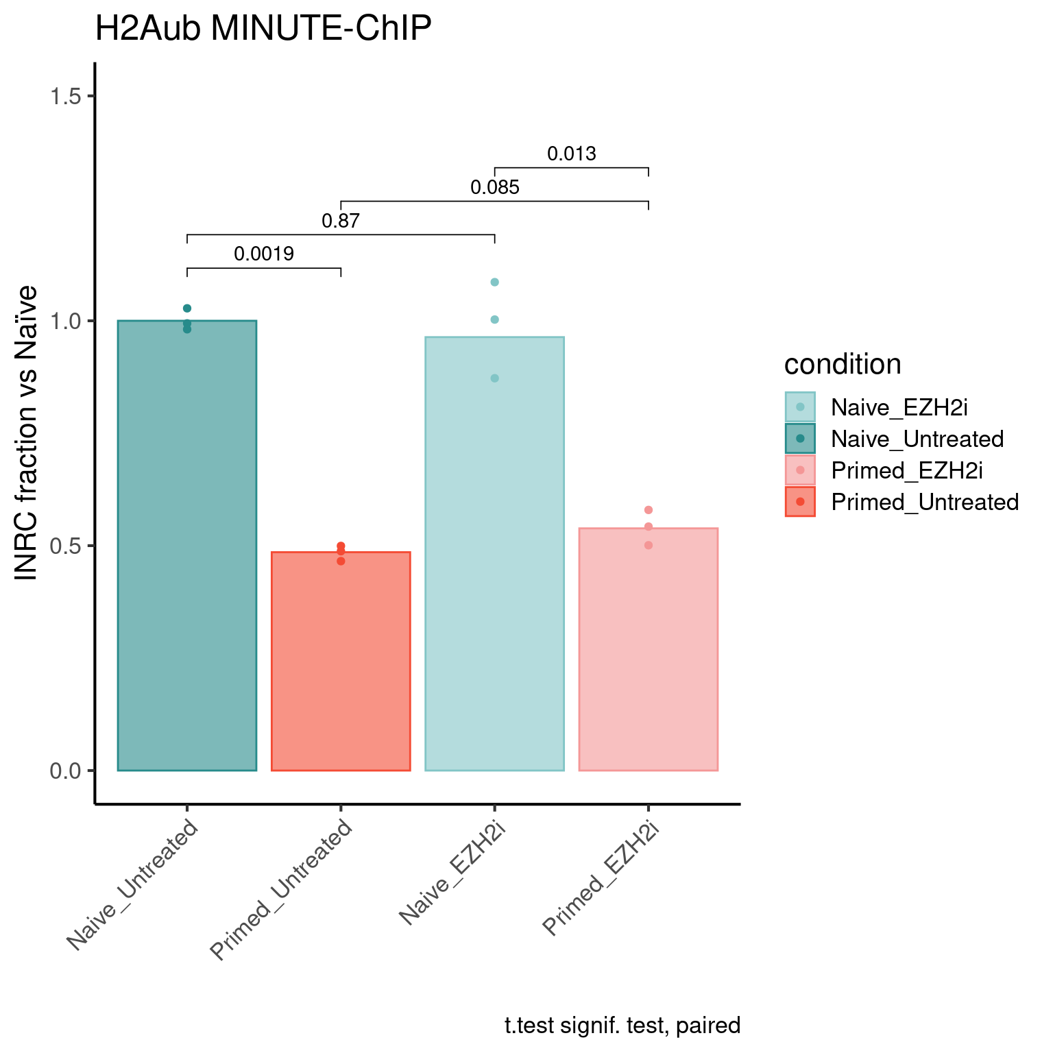
You can download data values here: download plot data.
H3K27m3 levels
inrc_barplot(inrc, "H3K27m3", colors_list)Warning: Removed 3 rows containing missing values (geom_signif).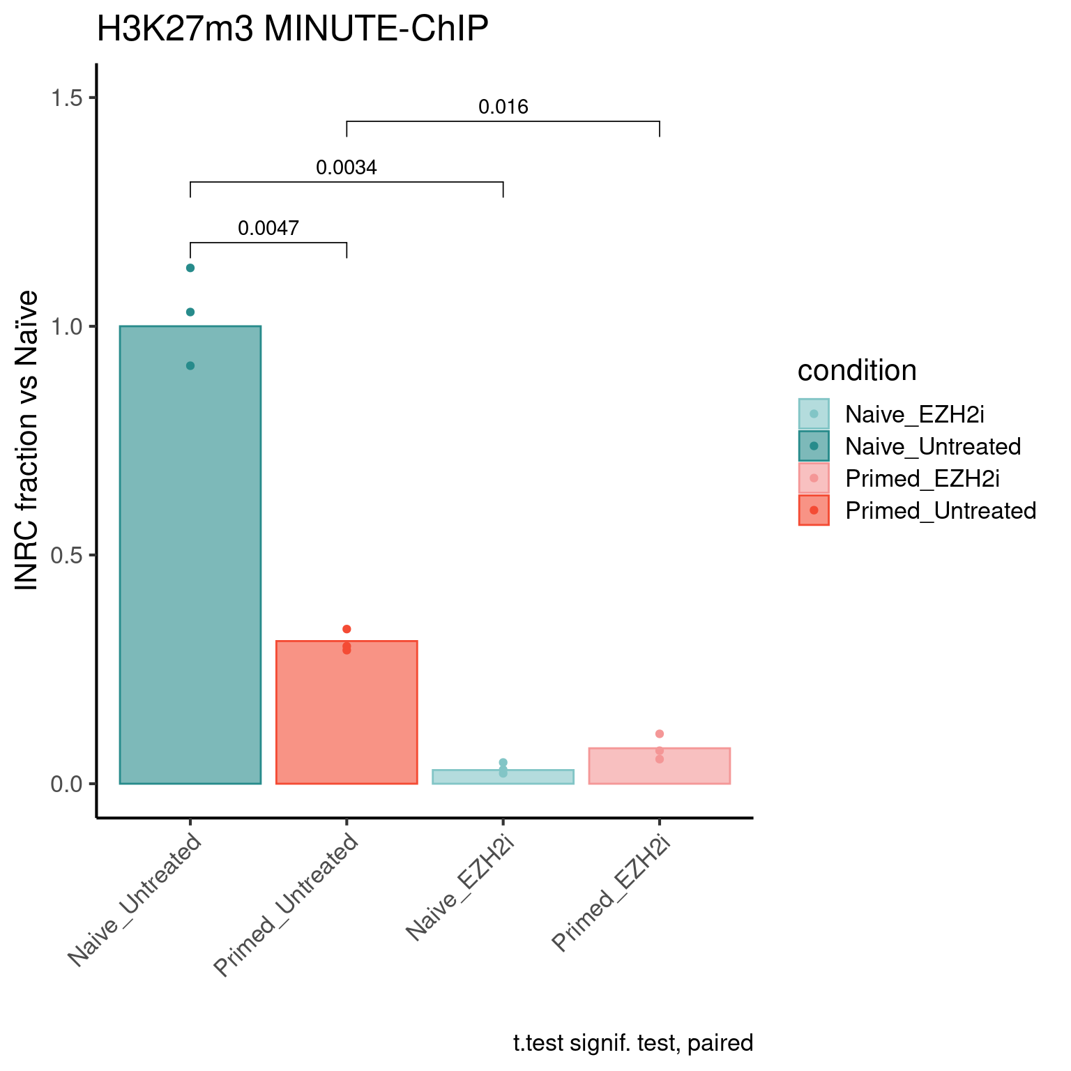
You can download data values here: download plot data.
H3K4m3 levels
inrc_barplot(inrc, "H3K4m3", colors_list)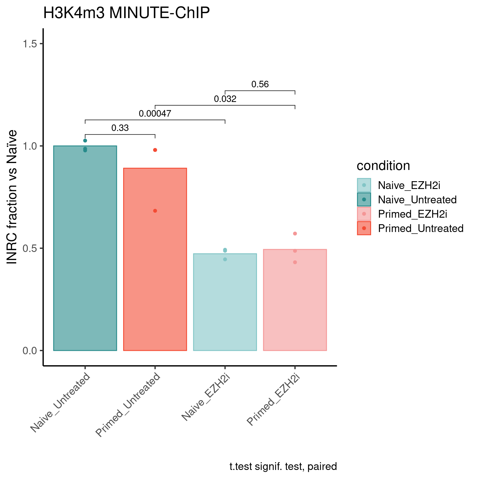
You can download data values here: download plot data.
ChromHMM global
Here global average per ChromHMM categories are shown.
H3K27m3
bwfiles <- list.files(file.path(params$datadir, "bw/Kumar_2020"), pattern = "H3K27m3.*pooled.*hg38.scaled", full.names = T)
labels <- gsub("_pooled.hg38.scaled.bw", "", basename(bwfiles))
labels <- gsub("_H9", "", labels)

chromhmm <- params$chromhmm

plot_bw_loci_summary_heatmap(bwfiles, chromhmm, labels = labels, remove_top=0.001)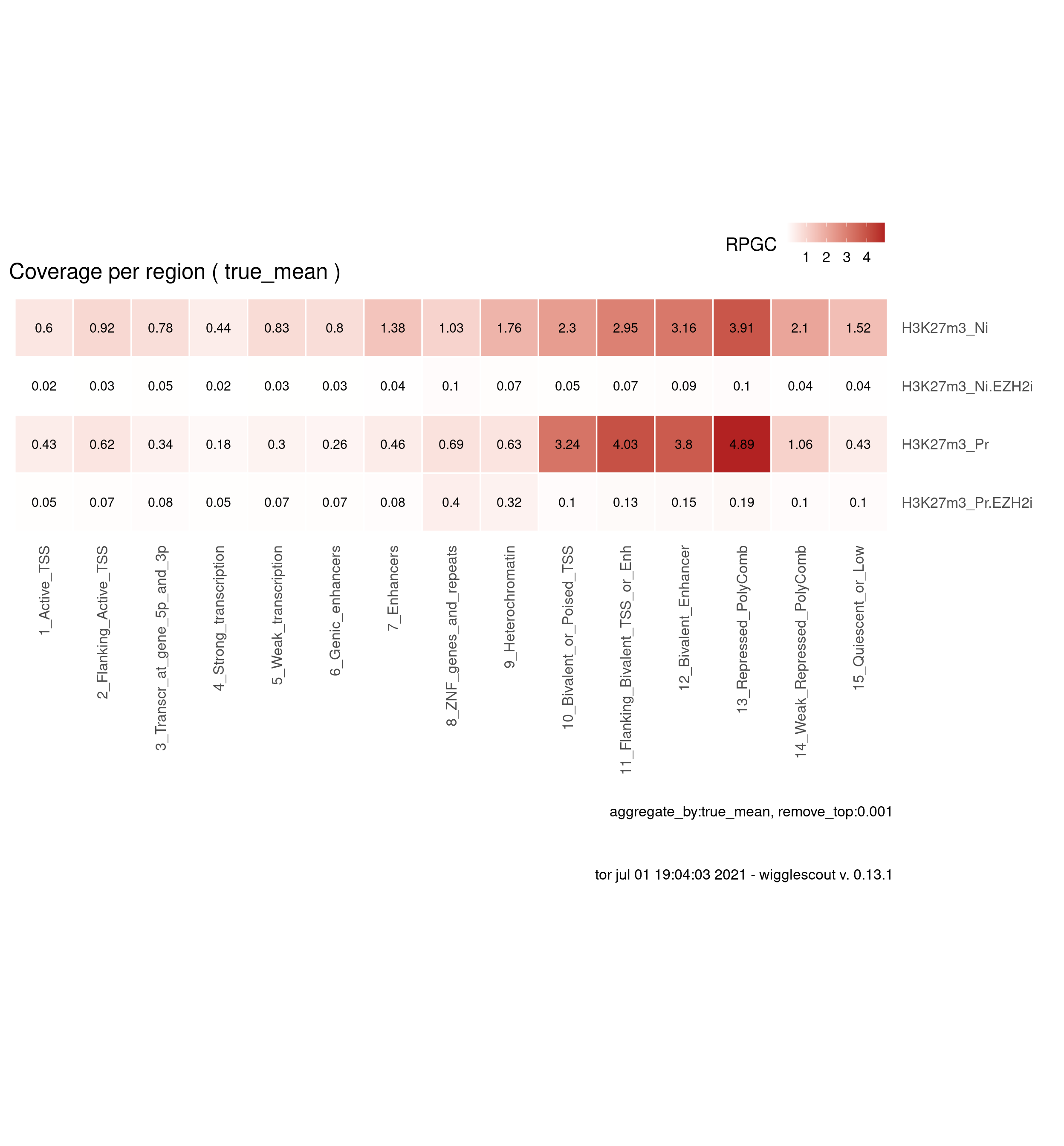
You can download data values here: download plot data.
H3K4m3
bwfiles <- list.files(file.path(params$datadir, "bw/Kumar_2020"), pattern = "H3K4m3.*pooled.*hg38.scaled", full.names = T)
labels <- gsub("_pooled.hg38.scaled.bw", "", basename(bwfiles))
labels <- gsub("_H9", "", labels)

plot_bw_loci_summary_heatmap(bwfiles, chromhmm, labels = labels, remove_top=0.001)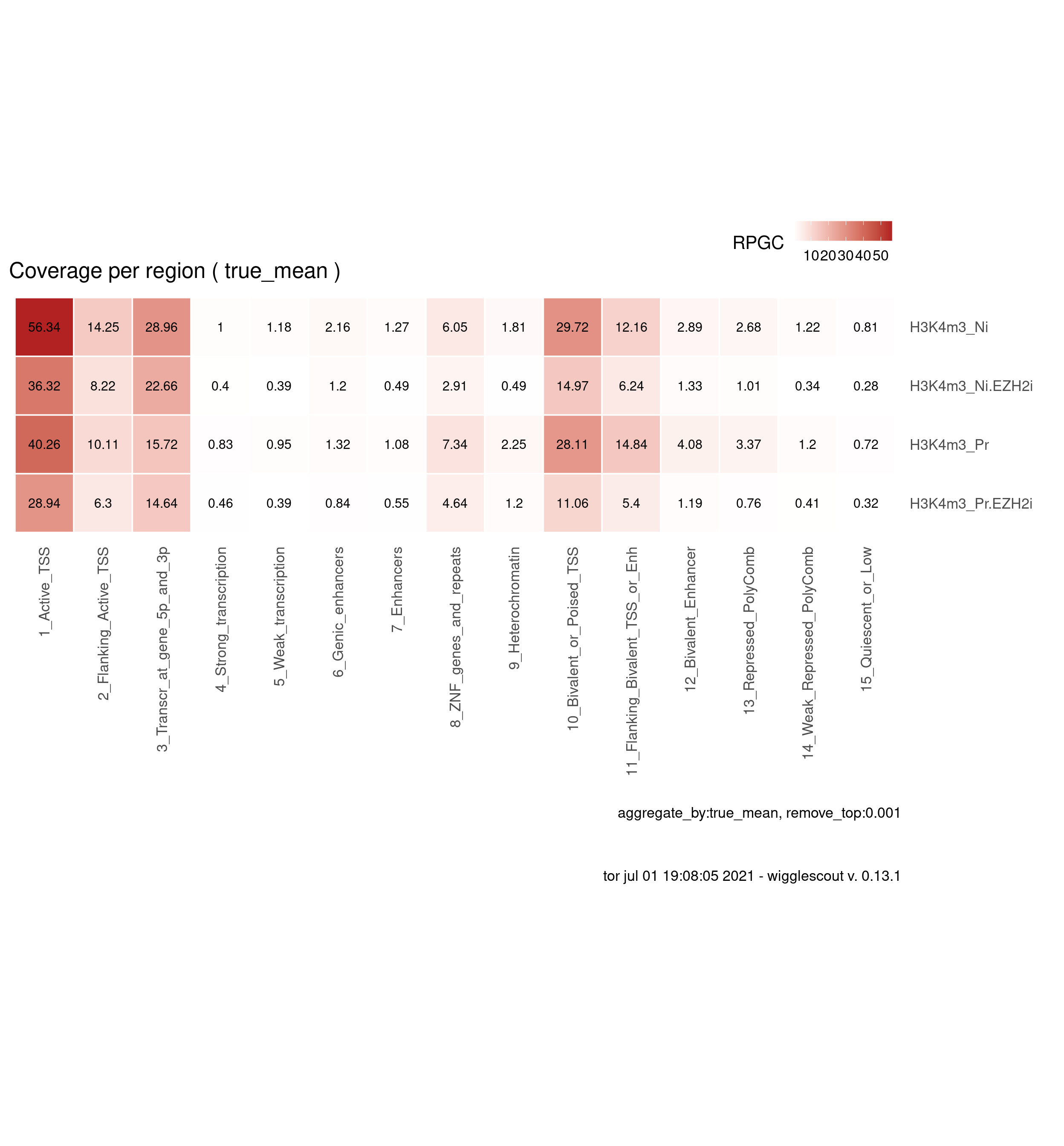
You can download data values here: download plot data.
H2AUb
bwfiles <- list.files(file.path(params$datadir, "bw/Kumar_2020"), pattern = "H2Aub.*pooled.*hg38.scaled", full.names = T)
labels <- gsub("_pooled.hg38.scaled.bw", "", basename(bwfiles))
labels <- gsub("_H9", "", labels)

chromhmm <- params$chromhmm

plot_bw_loci_summary_heatmap(bwfiles, chromhmm, labels = labels, remove_top=0.001)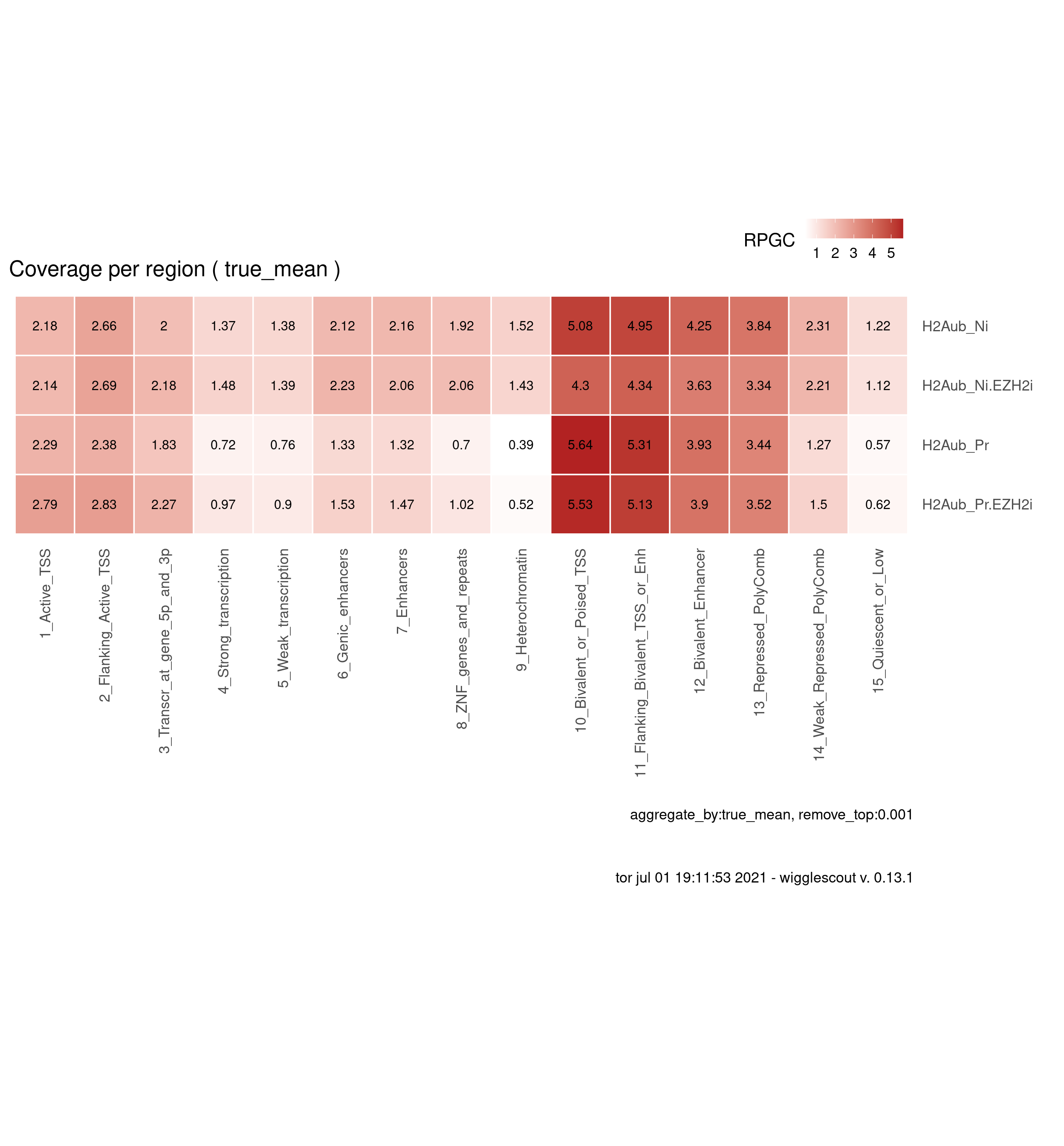
You can download data values here: download plot data.
sessionInfo()R version 4.1.0 (2021-05-18)
Platform: x86_64-pc-linux-gnu (64-bit)
Running under: Ubuntu 20.04.2 LTS
Matrix products: default
BLAS: /usr/lib/x86_64-linux-gnu/openblas-pthread/libblas.so.3
LAPACK: /usr/lib/x86_64-linux-gnu/openblas-pthread/liblapack.so.3
locale:
[1] LC_CTYPE=en_US.UTF-8 LC_NUMERIC=C
[3] LC_TIME=sv_SE.UTF-8 LC_COLLATE=en_US.UTF-8
[5] LC_MONETARY=sv_SE.UTF-8 LC_MESSAGES=en_US.UTF-8
[7] LC_PAPER=sv_SE.UTF-8 LC_NAME=C
[9] LC_ADDRESS=C LC_TELEPHONE=C
[11] LC_MEASUREMENT=sv_SE.UTF-8 LC_IDENTIFICATION=C
attached base packages:
[1] stats graphics grDevices utils datasets methods base
other attached packages:
[1] purrr_0.3.4 svglite_2.0.0 knitr_1.33 ggpubr_0.4.0
[5] dplyr_1.0.7 reshape2_1.4.4 ggplot2_3.3.5 wigglescout_0.13.1
[9] workflowr_1.6.2
loaded via a namespace (and not attached):
[1] bitops_1.0-7 matrixStats_0.59.0
[3] fs_1.5.0 RColorBrewer_1.1-2
[5] rprojroot_2.0.2 GenomeInfoDb_1.28.0
[7] tools_4.1.0 backports_1.2.1
[9] bslib_0.2.5.1 utf8_1.2.1
[11] R6_2.5.0 DBI_1.1.1
[13] BiocGenerics_0.38.0 colorspace_2.0-2
[15] withr_2.4.2 tidyselect_1.1.1
[17] curl_4.3.2 compiler_4.1.0
[19] git2r_0.28.0 Biobase_2.52.0
[21] DelayedArray_0.18.0 labeling_0.4.2
[23] rtracklayer_1.52.0 sass_0.4.0
[25] scales_1.1.1 askpass_1.1
[27] systemfonts_1.0.2 stringr_1.4.0
[29] digest_0.6.27 Rsamtools_2.8.0
[31] foreign_0.8-81 rmarkdown_2.9
[33] rio_0.5.27 XVector_0.32.0
[35] pkgconfig_2.0.3 htmltools_0.5.1.1
[37] parallelly_1.26.1 MatrixGenerics_1.4.0
[39] highr_0.9 readxl_1.3.1
[41] rlang_0.4.11 farver_2.1.0
[43] jquerylib_0.1.4 BiocIO_1.2.0
[45] generics_0.1.0 jsonlite_1.7.2
[47] BiocParallel_1.26.0 zip_2.2.0
[49] car_3.0-11 RCurl_1.98-1.3
[51] magrittr_2.0.1 GenomeInfoDbData_1.2.6
[53] Matrix_1.3-4 Rcpp_1.0.6
[55] munsell_0.5.0 S4Vectors_0.30.0
[57] fansi_0.5.0 abind_1.4-5
[59] lifecycle_1.0.0 furrr_0.2.3
[61] stringi_1.6.2 whisker_0.4
[63] yaml_2.2.1 carData_3.0-4
[65] SummarizedExperiment_1.22.0 zlibbioc_1.38.0
[67] plyr_1.8.6 grid_4.1.0
[69] parallel_4.1.0 listenv_0.8.0
[71] promises_1.2.0.1 forcats_0.5.1
[73] crayon_1.4.1 lattice_0.20-44
[75] haven_2.4.1 Biostrings_2.60.1
[77] hms_1.1.0 pillar_1.6.1
[79] GenomicRanges_1.44.0 rjson_0.2.20
[81] ggsignif_0.6.2 codetools_0.2-18
[83] stats4_4.1.0 XML_3.99-0.6
[85] glue_1.4.2 evaluate_0.14
[87] data.table_1.14.0 vctrs_0.3.8
[89] httpuv_1.6.1 cellranger_1.1.0
[91] openssl_1.4.4 gtable_0.3.0
[93] tidyr_1.1.3 future_1.21.0
[95] assertthat_0.2.1 openxlsx_4.2.4
[97] xfun_0.24 broom_0.7.8
[99] restfulr_0.0.13 rstatix_0.7.0
[101] later_1.2.0 tibble_3.1.2
[103] GenomicAlignments_1.28.0 IRanges_2.26.0
[105] globals_0.14.0 ellipsis_0.3.2