Genome annotations
Carmen Navarro
2021-02-16
Last updated: 2021-03-10
Checks: 6 1
Knit directory: hesc-epigenomics/
This reproducible R Markdown analysis was created with workflowr (version 1.6.2). The Checks tab describes the reproducibility checks that were applied when the results were created. The Past versions tab lists the development history.
The R Markdown is untracked by Git. To know which version of the R Markdown file created these results, you’ll want to first commit it to the Git repo. If you’re still working on the analysis, you can ignore this warning. When you’re finished, you can run wflow_publish to commit the R Markdown file and build the HTML.
Great job! The global environment was empty. Objects defined in the global environment can affect the analysis in your R Markdown file in unknown ways. For reproduciblity it’s best to always run the code in an empty environment.
The command set.seed(20210202) was run prior to running the code in the R Markdown file. Setting a seed ensures that any results that rely on randomness, e.g. subsampling or permutations, are reproducible.
Great job! Recording the operating system, R version, and package versions is critical for reproducibility.
Nice! There were no cached chunks for this analysis, so you can be confident that you successfully produced the results during this run.
Great job! Using relative paths to the files within your workflowr project makes it easier to run your code on other machines.
Great! You are using Git for version control. Tracking code development and connecting the code version to the results is critical for reproducibility.
The results in this page were generated with repository version cbc76ea. See the Past versions tab to see a history of the changes made to the R Markdown and HTML files.
Note that you need to be careful to ensure that all relevant files for the analysis have been committed to Git prior to generating the results (you can use wflow_publish or wflow_git_commit). workflowr only checks the R Markdown file, but you know if there are other scripts or data files that it depends on. Below is the status of the Git repository when the results were generated:
Ignored files:
    Ignored:    .Rhistory
    Ignored:    .Rproj.user/
    Ignored:    data/bed/
    Ignored:    data/bw
    Ignored:    data/meta/
    Ignored:    data/peaks
    Ignored:    data/rnaseq/

Untracked files:
    Untracked:  analysis/annotations.Rmd
    Untracked:  analysis/histone_marks_vs_expression.Rmd
    Untracked:  code/deseq_functions.R
    Untracked:  code/ucsc_annotations.R
    Untracked:  output/annotations/

Unstaged changes:
    Modified:   analysis/index.Rmd
    Modified:   code/embed_functions.R
Note that any generated files, e.g. HTML, png, CSS, etc., are not included in this status report because it is ok for generated content to have uncommitted changes.
There are no past versions. Publish this analysis with wflow_publish() to start tracking its development.
Summary
This notebook shows how the genome annotations relevant for this publication were calculated.
Gene annotation
Gene annotation is obtained from UCSC hg38 annotation.
genes <- genes_hg38()Only genes that have a gene symbol associated to it are kept, leaving a set of 25747.
Download gene annotation.
Bivalent genes by name
Bivalent genes are obtained from UCSC hg38 annotation using as names the ones in (Court and Arnaud 2017) supplementary table.
gene_file <- file.path(params$datadir, "meta/Court_2017_gene_names_uniq.txt")
gene_list <- read.table(gene_file, header=F)
colnames(gene_list) <- c("name")

biv_genes_name <- get_genes_by_name(gene_list$name)
From the list of 5378 gene names from (Court and Arnaud 2017), 3925 unique genomic loci are successfully retrieved.
Download bivalent gene annotation.
Download genes list.
Bivalent genes by overlap
Bivalent genes are obtained from overlap of hg38-liftovered from original (Court and Arnaud 2017) genes with UCSC hg38 annotation.
gene_file <- file.path(params$datadir, "bed/Bivalent_Court2017.hg38.bed")
gene_loci <- import(gene_file)

biv_genes_overlap <- get_genes_by_overlap(gene_loci)

export(biv_genes_overlap, "./data/bed/Court_2017_bivalent_genes.bed")
From the list of 5378 gene names from (Court and Arnaud 2017), 4874 unique genomic loci are successfully retrieved.
Download bivalent gene annotation.
Match between both
field_list <- list(names = biv_genes_name$name, overlap = biv_genes_overlap$name)
ggvenn(field_list, fill_alpha = 0.5, text_size = 5, stroke_color = "#ffffff") +
    ggtitle("Names vs location")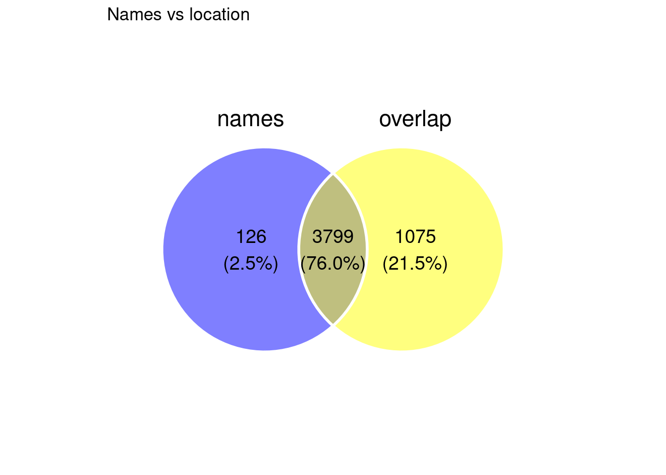
Some of the names cases are: either the gene has not been annotated because locus is proximal to annotation but not overlapping it (this may be because of lift over of coordinates), or because the name from UCSC hg38 annotation does not match the name in Court 2017 original annotated gene name.
H3K27m3 differential TSS
bw_cond_1 <-
  list.files(
    file.path(params$datadir, "bw/Kumar_2020/hu2"),
    full.names = T,
    pattern = "H3K27m3_H9_Ni_rep[1-3].hg38.scaled.bw"
  )
bw_cond_2 <-
  list.files(
    file.path(params$datadir, "bw/Kumar_2020/hu2"),
    full.names = T,
    pattern = "H3K27m3_H9_Pr_rep[1-3].hg38.scaled.bw"
  )

all_hg38_genes <- genes_hg38()
tss <- promoters(all_hg38_genes, upstream = 2500, downstream = 2500)
mcols(tss) <- NULL

c1 <- bw_loci(bw_cond_1, tss)
c2 <- bw_loci(bw_cond_2, tss)

diff <- bw_granges_diff_analysis(c2, c1, "Primed", "Naive", estimate_size_factors = FALSE)
diff_lfc <- lfcShrink(diff, coef="condition_Naive_vs_Primed", type="apeglm")

data <- plotMA(diff_lfc, returnData = T)

ggplot(data, aes(x=mean, y=lfc, color=isDE)) +
  geom_point(alpha=0.5, size=0.7) +
  theme_default() +
  scale_color_manual(values = list("FALSE"="grey", "TRUE"="red")) +
  geom_hline(yintercept = 0, linetype="dashed") +
  theme(legend.position = "none") +
  ggtitle("H3K27me3 diff. decorated TSS - All genes") + scale_x_log10() + ylim(-5, 5)
# select by cutoff
p_cutoff <- 0.05
diff_lfc <- diff_lfc[!is.na(diff_lfc$padj), ]
signif_tss <- diff_lfc[diff_lfc$padj <= p_cutoff & abs(diff_lfc$log2FoldChange) > 1, ]

mcols(c1) <- NULL
signif_gr <- c1[as.numeric(rownames(signif_tss)), ]
signif_gr$score <- signif_tss$log2FoldChange

export(signif_gr, "./data/bed/Kumar_2020_H3K27m3_diff_tss.bed")

# Select bivalent ones
signif_gr_biv <- subsetByOverlaps(biv_genes_overlap, signif_gr)
export(signif_gr_biv, "./data/bed/Kumar_2020_H3K27m3_diff_bivalent.bed")
Bivalent
biv_genes <- biv_genes_overlap
tss <- promoters(biv_genes, upstream = 2500, downstream = 2500)
tss$gene_id <- NULL

c1 <- bw_loci(bw_cond_1, tss)
c2 <- bw_loci(bw_cond_2, tss)

diff <- bw_granges_diff_analysis(c2, c1, "Primed", "Naive", estimate_size_factors = FALSE)
diff_lfc <- lfcShrink(diff, coef="condition_Naive_vs_Primed", type="apeglm")

data <- plotMA(diff_lfc, returnData = T)

ggplot(data, aes(x=mean, y=lfc, color=isDE)) +
  geom_point(alpha=0.8, size=0.8) +
  theme_default() +
  scale_color_manual(values = list("FALSE"="grey", "TRUE"="red")) +
  geom_hline(yintercept = 0, linetype="dashed") +
  theme(legend.position = "none") +
  ggtitle("H3K27me3 diff. decorated bivalent TSS") + scale_x_log10() + ylim(-5, 5)
# select by cutoff
p_cutoff <- 0.05
diff_lfc <- diff_lfc[!is.na(diff_lfc$padj), ]
signif_tss <- diff_lfc[diff_lfc$padj <= p_cutoff & abs(diff_lfc$log2FoldChange) > 1, ]

signif_gr <- c1[c1$name %in% rownames(signif_tss), ]

signif_gr$score <- signif_tss$log2FoldChange

export(signif_gr, "./data/bed/Kumar_2020_H3K27m3_diff_tss_bivalent.bed")
Compare
global <- import("./data/bed/Kumar_2020_H3K27m3_diff_bivalent_genes.bed")
local <- import("./data/bed/Kumar_2020_H3K27m3_diff_tss_bivalent.bed")
field_list <- list(global = global$name, local = local$name)
ggvenn(field_list, fill_alpha = 0.5, text_size = 5, stroke_color = "#ffffff") +
    ggtitle("Global vs local")
H2Aub differential TSS
bw_cond_1 <-
  list.files(
    file.path(params$datadir, "bw/Kumar_2020/hu2"),
    full.names = T,
    pattern = "H2Aub_H9_Ni_rep[1-3].hg38.scaled.bw"
  )
bw_cond_2 <-
  list.files(
    file.path(params$datadir, "bw/Kumar_2020/hu2"),
    full.names = T,
    pattern = "H2Aub_H9_Pr_rep[1-3].hg38.scaled.bw"
  )

all_hg38_genes <- genes_hg38()
tss <- promoters(all_hg38_genes, upstream = 1500, downstream = 1500)
mcols(tss) <- NULL

c1 <- bw_loci(bw_cond_1, tss)
c2 <- bw_loci(bw_cond_2, tss)

diff <- bw_granges_diff_analysis(c2, c1, "Primed", "Naive", estimate_size_factors = FALSE)
diff_lfc <- lfcShrink(diff, coef="condition_Naive_vs_Primed", type="apeglm")

data <- plotMA(diff_lfc, returnData = T)

ggplot(data, aes(x=mean, y=lfc, color=isDE)) +
  geom_point(alpha=0.5, size=0.7) +
  theme_default() +
  scale_color_manual(values = list("FALSE"="grey", "TRUE"="red")) +
  geom_hline(yintercept = 0, linetype="dashed") +
  theme(legend.position = "none") +
  ggtitle("H2Aub diff. decorated TSS - All genes") + scale_x_log10()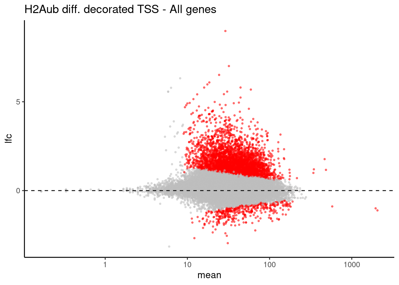
# select by cutoff
p_cutoff <- 0.05
diff_lfc <- diff_lfc[!is.na(diff_lfc$padj), ]
signif_tss <- diff_lfc[diff_lfc$padj <= p_cutoff & abs(diff_lfc$log2FoldChange) > 1, ]

mcols(c1) <- NULL
signif_gr <- c1[as.numeric(rownames(signif_tss)), ]
signif_gr$score <- signif_tss$log2FoldChange

export(signif_gr, "./data/bed/Kumar_2020_H2Aub_diff_tss.bed")

# Select bivalent ones
signif_gr_biv <- subsetByOverlaps(biv_genes_overlap, signif_gr)
export(signif_gr_biv, "./data/bed/Kumar_2020_H2Aub_diff_bivalent.bed")
H3K4m3 differential TSS
bw_cond_1 <-
  list.files(
    file.path(params$datadir, "bw/Kumar_2020/hu2"),
    full.names = T,
    pattern = "H3K4m3_H9_Ni_rep[1-3].hg38.scaled.bw"
  )
bw_cond_2 <-
  list.files(
    file.path(params$datadir, "bw/Kumar_2020/hu2"),
    full.names = T,
    pattern = "H3K4m3_H9_Pr_rep[1-3].hg38.scaled.bw"
  )

all_hg38_genes <- genes_hg38()
tss <- promoters(all_hg38_genes, upstream = 1500, downstream = 1500)
mcols(tss) <- NULL

c1 <- bw_loci(bw_cond_1, tss)
c2 <- bw_loci(bw_cond_2, tss)

diff <- bw_granges_diff_analysis(c2, c1, "Primed", "Naive", estimate_size_factors = FALSE)
diff_lfc <- lfcShrink(diff, coef="condition_Naive_vs_Primed", type="apeglm")

data <- plotMA(diff_lfc, returnData = T)

ggplot(data, aes(x=mean, y=lfc, color=isDE)) +
  geom_point(alpha=0.5, size=0.7) +
  theme_default() +
  scale_color_manual(values = list("FALSE"="grey", "TRUE"="red")) +
  geom_hline(yintercept = 0, linetype="dashed") +
  theme(legend.position = "none") +
  ggtitle("H3K4me3 diff. decorated TSS - All genes") + scale_x_log10()
# select by cutoff
p_cutoff <- 0.05
diff_lfc <- diff_lfc[!is.na(diff_lfc$padj), ]
signif_tss <- diff_lfc[diff_lfc$padj <= p_cutoff & abs(diff_lfc$log2FoldChange) > 1, ]

mcols(c1) <- NULL
signif_gr <- c1[as.numeric(rownames(signif_tss)), ]
signif_gr$score <- signif_tss$log2FoldChange

export(signif_gr, "./data/bed/Kumar_2020_H3K4m3_diff_tss.bed")

# Select bivalent ones
signif_gr_biv <- subsetByOverlaps(biv_genes_overlap, signif_gr)
export(signif_gr_biv, "./data/bed/Kumar_2020_H3K4m3_diff_bivalent.bed")
Genome-wide differential test annotation
H3K27m3 differential 5b bins
bw_cond_1 <-
  list.files(
    file.path(params$datadir, "bw/Kumar_2020/hu2"),
    full.names = T,
    pattern = "H3K27m3_H9_Ni_rep[1-3].hg38.scaled.bw"
  )
bw_cond_2 <-
  list.files(
    file.path(params$datadir, "bw/Kumar_2020/hu2"),
    full.names = T,
    pattern = "H3K27m3_H9_Pr_rep[1-3].hg38.scaled.bw"
  )

bs <- 5000
c1 <- bw_bins(bw_cond_1, bin_size = bs, genome = "hg38")
c2 <- bw_bins(bw_cond_2, bin_size = bs, genome = "hg38")

diff <- bw_granges_diff_analysis(c2, c1, "Primed", "Naive", estimate_size_factors = FALSE)
diff_lfc <- lfcShrink(diff, coef="condition_Naive_vs_Primed", type="apeglm")

mcols(c1) <- NULL
c1$logfc <- diff_lfc$log2FoldChange
c1$padj <- diff_lfc$padj

p_cutoff <- 0.05
c1$score <- 0
c1 <- c1[!is.na(c1$padj), ]
c1[c1$padj <= p_cutoff & c1$logfc > 0, ]$score <- 1
c1[c1$padj <= p_cutoff & c1$logfc < 0, ]$score <- -1
c1 <- c1[c1$padj <= p_cutoff]
export(c1, "./data/bed/Kumar_2020_H3K27m3_signif_ni_05_5kb.bed")
H3K4m3 differential 5kb bins
bw_cond_1 <-
  list.files(
    file.path(params$datadir, "bw/Kumar_2020/hu2"),
    full.names = T,
    pattern = "H3K4m3_H9_Ni_rep[1-3].hg38.scaled.bw"
  )
bw_cond_2 <-
  list.files(
    file.path(params$datadir, "bw/Kumar_2020/hu2"),
    full.names = T,
    pattern = "H3K4m3_H9_Pr_rep[1-3].hg38.scaled.bw"
  )

bs <- 5000
c1 <- bw_bins(bw_cond_1, bin_size = bs, genome = "hg38")
c2 <- bw_bins(bw_cond_2, bin_size = bs, genome = "hg38")

diff <- bw_granges_diff_analysis(c2, c1, "Primed", "Naive", estimate_size_factors = FALSE)
diff_lfc <- lfcShrink(diff, coef="condition_Naive_vs_Primed", type="apeglm")

mcols(c1) <- NULL
c1$logfc <- diff_lfc$log2FoldChange
c1$padj <- diff_lfc$padj

p_cutoff <- 0.05
c1$score <- 0
c1 <- c1[!is.na(c1$padj), ]
c1[c1$padj <= p_cutoff & c1$logfc > 0, ]$score <- 1
c1[c1$padj <= p_cutoff & c1$logfc < 0, ]$score <- -1
c1 <- c1[c1$padj <= p_cutoff]
export(c1, "./data/bed/Kumar_2020_H3K4m3_signif_ni_05_5kb.bed")
H2AUb differential 5kb bins
bw_cond_1 <-
  list.files(
    file.path(params$datadir, "bw/Kumar_2020/hu2"),
    full.names = T,
    pattern = "H2Aub_H9_Ni_rep[1-3].hg38.scaled.bw"
  )
bw_cond_2 <-
  list.files(
    file.path(params$datadir, "bw/Kumar_2020/hu2"),
    full.names = T,
    pattern = "H2Aub_H9_Pr_rep[1-3].hg38.scaled.bw"
  )

bs <- 5000
c1 <- bw_bins(bw_cond_1, bin_size = bs, genome = "hg38")
c2 <- bw_bins(bw_cond_2, bin_size = bs, genome = "hg38")

diff <- bw_granges_diff_analysis(c2, c1, "Primed", "Naive", estimate_size_factors = FALSE)
diff_lfc <- lfcShrink(diff, coef="condition_Naive_vs_Primed", type="apeglm")

mcols(c1) <- NULL
c1$logfc <- diff_lfc$log2FoldChange
c1$padj <- diff_lfc$padj

p_cutoff <- 0.05
c1$score <- 0
c1 <- c1[!is.na(c1$padj), ]
c1[c1$padj <= p_cutoff & c1$logfc > 0, ]$score <- 1
c1[c1$padj <= p_cutoff & c1$logfc < 0, ]$score <- -1
c1 <- c1[c1$padj <= p_cutoff]
export(c1, "./data/bed/Kumar_2020_H2AUb_signif_ni_05_5kb.bed")
Gene expression levels on Naïve and Primed hESC cells
Data: Used public data from (Collier et al. 2017): H9 embryonic stem cells in Naïve and Primed state, three biological replicates.
| dataset_id | gsm_id | description | filename | run_id | input | layout | experiment | |
|---|---|---|---|---|---|---|---|---|
| 26 | Collier_2017 | GSM2449055 | hESC_H9_naive_1 | hESC_H9_naive_1 | SRR5151102 | - | single | RNA-seq |
| 27 | Collier_2017 | GSM2449056 | hESC_H9_naive_2 | hESC_H9_naive_2 | SRR5151103 | - | single | RNA-seq |
| 28 | Collier_2017 | GSM2449057 | hESC_H9_naive_3 | hESC_H9_naive_3 | SRR5151104 | - | single | RNA-seq |
| 29 | Collier_2017 | GSM2449058 | hESC_H9_primed_1 | hESC_H9_primed_1 | SRR5151105 | - | single | RNA-seq |
| 30 | Collier_2017 | GSM2449059 | hESC_H9_primed_2 | hESC_H9_primed_2 | SRR5151106 | - | single | RNA-seq |
| 31 | Collier_2017 | GSM2449060 | hESC_H9_primed_3 | hESC_H9_primed_3 | SRR5151107 | - | single | RNA-seq |
sessionInfo()R version 4.0.4 (2021-02-15)
Platform: x86_64-pc-linux-gnu (64-bit)
Running under: Ubuntu 20.04.2 LTS
Matrix products: default
BLAS: /usr/lib/x86_64-linux-gnu/openblas-pthread/libblas.so.3
LAPACK: /usr/lib/x86_64-linux-gnu/openblas-pthread/liblapack.so.3
locale:
[1] LC_CTYPE=en_US.UTF-8 LC_NUMERIC=C
[3] LC_TIME=sv_SE.UTF-8 LC_COLLATE=en_US.UTF-8
[5] LC_MONETARY=sv_SE.UTF-8 LC_MESSAGES=en_US.UTF-8
[7] LC_PAPER=sv_SE.UTF-8 LC_NAME=C
[9] LC_ADDRESS=C LC_TELEPHONE=C
[11] LC_MEASUREMENT=sv_SE.UTF-8 LC_IDENTIFICATION=C
attached base packages:
[1] stats4 parallel grid stats graphics grDevices utils
[8] datasets methods base
other attached packages:
[1] DESeq2_1.30.0
[2] SummarizedExperiment_1.20.0
[3] MatrixGenerics_1.2.0
[4] matrixStats_0.58.0
[5] tidyr_1.1.2
[6] cowplot_1.1.1
[7] xfun_0.21
[8] purrr_0.3.4
[9] rtracklayer_1.50.0
[10] org.Hs.eg.db_3.11.4
[11] TxDb.Hsapiens.UCSC.hg38.knownGene_3.10.0
[12] GenomicFeatures_1.40.1
[13] AnnotationDbi_1.52.0
[14] Biobase_2.50.0
[15] GenomicRanges_1.42.0
[16] GenomeInfoDb_1.26.2
[17] IRanges_2.24.1
[18] S4Vectors_0.28.1
[19] BiocGenerics_0.36.0
[20] ggvenn_0.1.8
[21] dplyr_1.0.4
[22] knitr_1.31
[23] ggplot2_3.3.3
[24] wigglescout_0.12.8
[25] workflowr_1.6.2
loaded via a namespace (and not attached):
[1] colorspace_2.0-0 ellipsis_0.3.1 rprojroot_2.0.2
[4] XVector_0.30.0 fs_1.5.0 listenv_0.8.0
[7] furrr_0.2.2 farver_2.0.3 bit64_4.0.5
[10] mvtnorm_1.1-1 apeglm_1.10.0 xml2_1.3.2
[13] codetools_0.2-18 splines_4.0.4 cachem_1.0.4
[16] geneplotter_1.68.0 Rsamtools_2.6.0 annotate_1.68.0
[19] dbplyr_2.1.0 compiler_4.0.4 httr_1.4.2
[22] assertthat_0.2.1 Matrix_1.3-2 fastmap_1.1.0
[25] later_1.1.0.1 htmltools_0.5.1.1 prettyunits_1.1.1
[28] tools_4.0.4 coda_0.19-4 gtable_0.3.0
[31] glue_1.4.2 GenomeInfoDbData_1.2.4 reshape2_1.4.4
[34] rappdirs_0.3.3 Rcpp_1.0.6 bbmle_1.0.23.1
[37] vctrs_0.3.6 Biostrings_2.58.0 stringr_1.4.0
[40] globals_0.14.0 lifecycle_1.0.0 XML_3.99-0.5
[43] future_1.21.0 zlibbioc_1.36.0 MASS_7.3-53.1
[46] scales_1.1.1 hms_1.0.0 promises_1.2.0.1
[49] RColorBrewer_1.1-2 yaml_2.2.1 curl_4.3
[52] memoise_2.0.0 emdbook_1.3.12 bdsmatrix_1.3-4
[55] biomaRt_2.44.4 stringi_1.5.3 RSQLite_2.2.3
[58] highr_0.8 genefilter_1.72.0 BiocParallel_1.24.1
[61] rlang_0.4.10 pkgconfig_2.0.3 bitops_1.0-6
[64] evaluate_0.14 lattice_0.20-41 GenomicAlignments_1.26.0
[67] labeling_0.4.2 bit_4.0.4 tidyselect_1.1.0
[70] parallelly_1.23.0 plyr_1.8.6 magrittr_2.0.1
[73] R6_2.5.0 generics_0.1.0 DelayedArray_0.16.0
[76] DBI_1.1.1 pillar_1.4.7 withr_2.4.1
[79] survival_3.2-7 RCurl_1.98-1.2 tibble_3.0.6
[82] crayon_1.4.1 BiocFileCache_1.12.1 rmarkdown_2.6
[85] progress_1.2.2 locfit_1.5-9.4 blob_1.2.1
[88] git2r_0.28.0 digest_0.6.27 xtable_1.8-4
[91] numDeriv_2016.8-1.1 httpuv_1.5.5 openssl_1.4.3
[94] munsell_0.5.0 askpass_1.1