RUVs
Last updated: 2026-01-06
Checks: 7 0
Knit directory: DXR_website/
This reproducible R Markdown analysis was created with workflowr (version 1.7.1). The Checks tab describes the reproducibility checks that were applied when the results were created. The Past versions tab lists the development history.
Great! Since the R Markdown file has been committed to the Git repository, you know the exact version of the code that produced these results.
Great job! The global environment was empty. Objects defined in the global environment can affect the analysis in your R Markdown file in unknown ways. For reproduciblity it’s best to always run the code in an empty environment.
The command set.seed(20251201) was run prior to running
the code in the R Markdown file. Setting a seed ensures that any results
that rely on randomness, e.g. subsampling or permutations, are
reproducible.
Great job! Recording the operating system, R version, and package versions is critical for reproducibility.
Nice! There were no cached chunks for this analysis, so you can be confident that you successfully produced the results during this run.
Great job! Using relative paths to the files within your workflowr project makes it easier to run your code on other machines.
Great! You are using Git for version control. Tracking code development and connecting the code version to the results is critical for reproducibility.
The results in this page were generated with repository version e4705f6. See the Past versions tab to see a history of the changes made to the R Markdown and HTML files.
Note that you need to be careful to ensure that all relevant files for
the analysis have been committed to Git prior to generating the results
(you can use wflow_publish or
wflow_git_commit). workflowr only checks the R Markdown
file, but you know if there are other scripts or data files that it
depends on. Below is the status of the Git repository when the results
were generated:
Ignored files:
    Ignored:    .Rhistory
    Ignored:    .Rproj.user/
    Ignored:    DXR_website/data/
    Ignored:    code/Flow_Purity_Stressor_Boxplots_EMP_250226.R
    Ignored:    data/CDKN1A_geneplot_Dox.RDS
    Ignored:    data/Cormotif_dox.RDS
    Ignored:    data/Cormotif_prob_gene_list.RDS
    Ignored:    data/Cormotif_prob_gene_list_doxonly.RDS
    Ignored:    data/Counts_RNA_EMPfortmiller.txt
    Ignored:    data/DMSO_TNN13_plot.RDS
    Ignored:    data/DOX_TNN13_plot.RDS
    Ignored:    data/DOXgeneplots.RDS
    Ignored:    data/ExpressionMatrix_EMP.csv
    Ignored:    data/Ind1_DOX_Spearman_plot.RDS
    Ignored:    data/Ind6REP_Spearman_list.csv
    Ignored:    data/Ind6REP_Spearman_plot.RDS
    Ignored:    data/Ind6REP_Spearman_set.csv
    Ignored:    data/Ind6_Spearman_plot.RDS
    Ignored:    data/MDM2_geneplot_Dox.RDS
    Ignored:    data/Master_summary_75-1_EMP_250811_final.csv
    Ignored:    data/Master_summary_87-1_EMP_250811_final.csv
    Ignored:    data/Metadata.csv
    Ignored:    data/Metadata_2_norep_update.RDS
    Ignored:    data/Metadata_update.csv
    Ignored:    data/QC/
    Ignored:    data/Recovery_flow_purity.csv
    Ignored:    data/SIRT1_geneplot_Dox.RDS
    Ignored:    data/Sample_annotated.csv
    Ignored:    data/SpearmanHeatmapMatrix_EMP
    Ignored:    data/VolcanoPlot_D144R_original_EMP_250623.png
    Ignored:    data/VolcanoPlot_D24R_original_EMP_250623.png
    Ignored:    data/VolcanoPlot_D24T_original_EMP_250623.png
    Ignored:    data/annot_dox.RDS
    Ignored:    data/annot_list_hm.csv
    Ignored:    data/cormotif_dxr_1.RDS
    Ignored:    data/cormotif_dxr_2.RDS
    Ignored:    data/counts/
    Ignored:    data/counts_DE_df_dox.RDS
    Ignored:    data/counts_DE_raw_data.RDS
    Ignored:    data/counts_raw_filt.RDS
    Ignored:    data/counts_raw_matrix.RDS
    Ignored:    data/counts_raw_matrix_EMP_250514.csv
    Ignored:    data/d24_Spearman_plot.RDS
    Ignored:    data/dge_calc_dxr.RDS
    Ignored:    data/dge_calc_matrix.RDS
    Ignored:    data/ensembl_backup_dox.RDS
    Ignored:    data/fC_AllCounts.RDS
    Ignored:    data/fC_DOXCounts.RDS
    Ignored:    data/featureCounts_Concat_Matrix_DOXSamples_EMP_250430.csv
    Ignored:    data/featureCounts_DOXdata_updatedind.RDS
    Ignored:    data/filcpm_colnames_matrix.csv
    Ignored:    data/filcpm_matrix.csv
    Ignored:    data/filt_gene_list_dox.RDS
    Ignored:    data/filter_gene_list_final.RDS
    Ignored:    data/final_data/
    Ignored:    data/gene_clustlike_motif.RDS
    Ignored:    data/gene_postprob_motif.RDS
    Ignored:    data/genedf_dxr.RDS
    Ignored:    data/genematrix_dox.RDS
    Ignored:    data/genematrix_dxr.RDS
    Ignored:    data/heartgenes.csv
    Ignored:    data/heartgenes_dox.csv
    Ignored:    data/image_intensity_stats_all_conditions.csv
    Ignored:    data/image_level_stats_all_conditions.csv
    Ignored:    data/image_level_summary_yH2AX_quant.csv
    Ignored:    data/ind_num_dox.RDS
    Ignored:    data/ind_num_dxr.RDS
    Ignored:    data/initial_cormotif.RDS
    Ignored:    data/initial_cormotif_dox.RDS
    Ignored:    data/low_nuclei_samples.csv
    Ignored:    data/low_veh_samples.csv
    Ignored:    data/new/
    Ignored:    data/new_cormotif_dox.RDS
    Ignored:    data/perc_mean_all_10X.png
    Ignored:    data/perc_mean_all_20X.png
    Ignored:    data/perc_mean_all_40X.png
    Ignored:    data/perc_mean_consistent_10X.png
    Ignored:    data/perc_mean_consistent_20X.png
    Ignored:    data/perc_mean_consistent_40X.png
    Ignored:    data/perc_median_all_10X.png
    Ignored:    data/perc_median_all_20X.png
    Ignored:    data/perc_median_all_40X.png
    Ignored:    data/perc_median_consistent_10X.png
    Ignored:    data/perc_median_consistent_20X.png
    Ignored:    data/perc_median_consistent_40X.png
    Ignored:    data/plot_leg_d.RDS
    Ignored:    data/plot_leg_d_horizontal.RDS
    Ignored:    data/plot_leg_d_vertical.RDS
    Ignored:    data/plot_theme_custom.RDS
    Ignored:    data/process_gene_data_funct.RDS
    Ignored:    data/raw_mean_all_10X.png
    Ignored:    data/raw_mean_all_20X.png
    Ignored:    data/raw_mean_all_40X.png
    Ignored:    data/raw_mean_consistent_10X.png
    Ignored:    data/raw_mean_consistent_20X.png
    Ignored:    data/raw_mean_consistent_40X.png
    Ignored:    data/raw_median_all_10X.png
    Ignored:    data/raw_median_all_20X.png
    Ignored:    data/raw_median_all_40X.png
    Ignored:    data/raw_median_consistent_10X.png
    Ignored:    data/raw_median_consistent_20X.png
    Ignored:    data/raw_median_consistent_40X.png
    Ignored:    data/ruv/
    Ignored:    data/summary_all_IF_ROI.RDS
    Ignored:    data/tableED_GOBP.RDS
    Ignored:    data/tableESR_GOBP_postprob.RDS
    Ignored:    data/tableLD_GOBP.RDS
    Ignored:    data/tableLR_GOBP_postprob.RDS
    Ignored:    data/tableNR_GOBP.RDS
    Ignored:    data/tableNR_GOBP_postprob.RDS
    Ignored:    data/table_incsus_genes_GOBP_RUV.RDS
    Ignored:    data/table_motif1_GOBP_d.RDS
    Ignored:    data/table_motif1_genes_GOBP.RDS
    Ignored:    data/table_motif2_GOBP_d.RDS
    Ignored:    data/table_motif3_genes_GOBP.RDS
    Ignored:    data/thing.R
    Ignored:    data/top.table_V.D144r_dox.RDS
    Ignored:    data/top.table_V.D24_dox.RDS
    Ignored:    data/top.table_V.D24r_dox.RDS
    Ignored:    data/yH2AX_75-1_EMP_250811.csv
    Ignored:    data/yH2AX_87-1_EMP_250811.csv
    Ignored:    data/yH2AX_Boxplots_MeanIntensity_10X_EMP_250811.png
    Ignored:    data/yH2AX_Boxplots_MeanIntensity_10X_NormtoMax_EMP_250811.png
    Ignored:    data/yH2AX_Boxplots_MeanIntensity_20X_EMP_250811.png
    Ignored:    data/yH2AX_Boxplots_MeanIntensity_20X_NormtoMax_EMP_250811.png
    Ignored:    data/yH2AX_Boxplots_MedianIntensity_10X_NormtoMax_EMP_250811.png
    Ignored:    data/yH2AX_Boxplots_MedianIntensity_20X_NormtoMax_EMP_250811.png
    Ignored:    data/yH2AX_Boxplots_MedianIntensity_NormtoMax_EMP_250811.png
    Ignored:    data/yH2AX_Boxplots_Quant_10X_EMP_250817.png
    Ignored:    data/yH2AX_Boxplots_Quant_20X_EMP_250817.png
    Ignored:    data/yh2ax_all_df_EMP_250812.csv
Note that any generated files, e.g. HTML, png, CSS, etc., are not included in this status report because it is ok for generated content to have uncommitted changes.
These are the previous versions of the repository in which changes were
made to the R Markdown (DXR_website/analysis/RUVs.Rmd) and
HTML (DXR_website/docs/RUVs.html) files. If you’ve
configured a remote Git repository (see ?wflow_git_remote),
click on the hyperlinks in the table below to view the files as they
were in that past version.
| File | Version | Author | Date | Message |
|---|---|---|---|---|
| html | c382b38 | emmapfort | 2026-01-06 | Build site. |
| Rmd | cd535e9 | emmapfort | 2026-01-06 | Final Website Touches 01/06/25 EMP |
| html | 7f22593 | emmapfort | 2026-01-05 | Build site. |
| Rmd | 49fa865 | emmapfort | 2026-01-05 | Final Updates to Website EMP 01/05/26 |
| html | 1100814 | emmapfort | 2025-12-09 | Build site. |
| Rmd | a967d53 | emmapfort | 2025-12-09 | Update website and analysis chunks |
| html | a967d53 | emmapfort | 2025-12-09 | Update website and analysis chunks |
Libraries
Load necessary libraries for analysis.
library(RUVSeq)
library(tidyverse)
library(readr)
library(readxl)
library(edgeR)
library(ggfortify)
library(ComplexHeatmap)
library(ggrepel)
Define my custom plot theme
# Define the custom theme
# plot_theme_custom <- function() {
#   theme_minimal() +
#     theme(
#       #line for x and y axis
#       axis.line = element_line(linewidth = 1,
#                                color = "black"),
#
#       #axis ticks only on x and y, length standard
#       axis.ticks.x = element_line(color = "black",
#                                 linewidth = 1),
#       axis.ticks.y = element_line(color = "black",
#                                 linewidth = 1),
#       axis.ticks.length = unit(0.05, "in"),
#
#       #text and font
#       axis.text = element_text(color = "black",
#                                family = "Arial",
#                                size = 7),
#       axis.title = element_text(color = "black",
#                                 family = "Arial",
#                                 size = 9),
#       legend.text = element_text(color = "black",
#                                  family = "Arial",
#                                  size = 7),
#       legend.title = element_text(color = "black",
#                                   family = "Arial",
#                                   size = 9),
#       plot.title = element_text(color = "black",
#                                 family = "Arial",
#                                 size = 10),
#
#       #blank background and border
#       panel.background = element_blank(),
#       panel.border = element_blank(),
#
#       #gridlines for alignment
#       panel.grid.major = element_line(color = "grey80", linewidth = 0.5),  #grey major grid for align in illus
#       panel.grid.minor = element_line(color = "grey90", linewidth = 0.5) #grey minor grid for align in illus
#     )
# }

# saveRDS(plot_theme_custom, "data/plot_theme_custom.RDS")

theme_custom <- readRDS("data/plot_theme_custom.RDS")
Factors and Colors
Include each of the factors for these experiments as well as their color schemes.
####Colors####

# txtime_col_old <- list(
#   "DOX_24T" = "#263CA5",
#   "VEH_24T" = "#444343",
#   "DOX_24R" = "#5B8FD1",
#   "VEH_24R" = "#757575",
#   "DOX_144R" = "#89C5E5",
#   "VEH_144R" = "#AAAAAA"
# )

#updated colors and factors:
ind_col <- list(
  "1" = "#FF9F64",
  "2" = "#78EBDA",
  "3" = "#ADCD77",
  "4" = "#E6CC50",
  "5" = "#A68AC0",
  "6" = "#F16F90",
  "6R" = "#C61E4E"
)

ind_col_nr <- list(
  "1" = "#FF9F64",
  "2" = "#78EBDA",
  "3" = "#ADCD77",
  "4" = "#E6CC50",
  "5" = "#A68AC0",
  "6" = "#F16F90"
)

time_col <- list(
  "t0" = "#005A4C",
  "t24" = "#328477",
  "t144" = "#8FB9B1")

tx_col <- list(
  "DOX" = "#499FBD",
  "VEH" = "#BBBBBC")

txtime_col <- list(
  "DOX_t0" = "#263CA5",
  "VEH_t0" = "#444343",
  "DOX_t24" = "#5B8FD1",
  "VEH_t24" = "#757575",
  "DOX_t144" = "#89C5E5",
  "VEH_t144" = "#AAAAAA"
)
Saving plots function
Define a function to save plots as .pdf and .png
save_plot <- function(plot, filename,
                      folder = ".",
                      width = 8,
                      height = 6,
                      units = "in",
                      dpi = 300,
                      add_date = TRUE) {
  if (missing(filename)) stop("Please provide a filename (without extension) for the plot.")

  date_str <- if (add_date) paste0("_", format(Sys.Date(), "%y%m%d")) else ""
  pdf_file <- file.path(folder, paste0(filename, date_str, ".pdf"))
  png_file <- file.path(folder, paste0(filename, date_str, ".png"))
  ggsave(filename = pdf_file, plot = plot, device = cairo_pdf, width = width, height = height, units = units, bg = "transparent")
  ggsave(filename = png_file, plot = plot, device = "png", width = width, height = height, units = units, dpi = dpi, bg = "transparent")
  message("Saved plot as Cairo PDF: ", pdf_file)
  message("Saved plot as PNG: ", png_file)
}

output_folder <- "C:/Users/emmap/OneDrive/Desktop/DXR Manuscript Materials/Fig pdfs"


#save plot function created
#to use: just define the plot name, filename_base, width, height
Principal Component Analysis
Identify principal components contributing to variation in the data.
#Now I want to check if my data is as expected on a PCA plot
counts_cpm_unfilt <- readRDS("data/QC/counts_cpm_unfilt.RDS")
filcpm_matrix <- readRDS("data/QC/filcpm_final_matrix_newind.RDS")

#perform PCA calculations
prcomp_res_unfilt <- prcomp(t(counts_cpm_unfilt %>% as.matrix()), center =  TRUE)

prcomp_res_filt <- prcomp(t(filcpm_matrix %>% as.matrix()), center =  TRUE)

#read in my metadata annotations
#this has already had the individual number changed to move 84-1

Metadata <- read.csv("data/QC/Metadata_update.csv") %>%
  dplyr::select(-X)
#84-1 is now Ind4


#add in labels for individual numbers
ind_num <- c("1", "1", "1", "1", "1", "1",
             "2", "2", "2", "2", "2", "2",
             "3", "3", "3", "3", "3", "3",
             "4", "4", "4", "4", "4", "4",
             "5", "5", "5", "5", "5", "5",
             "6", "6", "6", "6", "6", "6",
             "6R", "6R", "6R", "6R", "6R", "6R")

# saveRDS(ind_num, "data/QC/ind_num.RDS")


#now plot my PCA for unfiltered log2cpm
####PC1/PC2####
ggplot2::autoplot(prcomp_res_unfilt, data = Metadata, colour = "Cond", shape = "Time", size =4, x=1, y=2) +
  ggrepel::geom_text_repel(label=ind_num, vjust = -.5, max.overlaps = 30) +
  scale_color_manual(values=txtime_col) +
  ggtitle(expression("PCA of Unfiltered log"[2]*"cpm")) +
  theme_custom()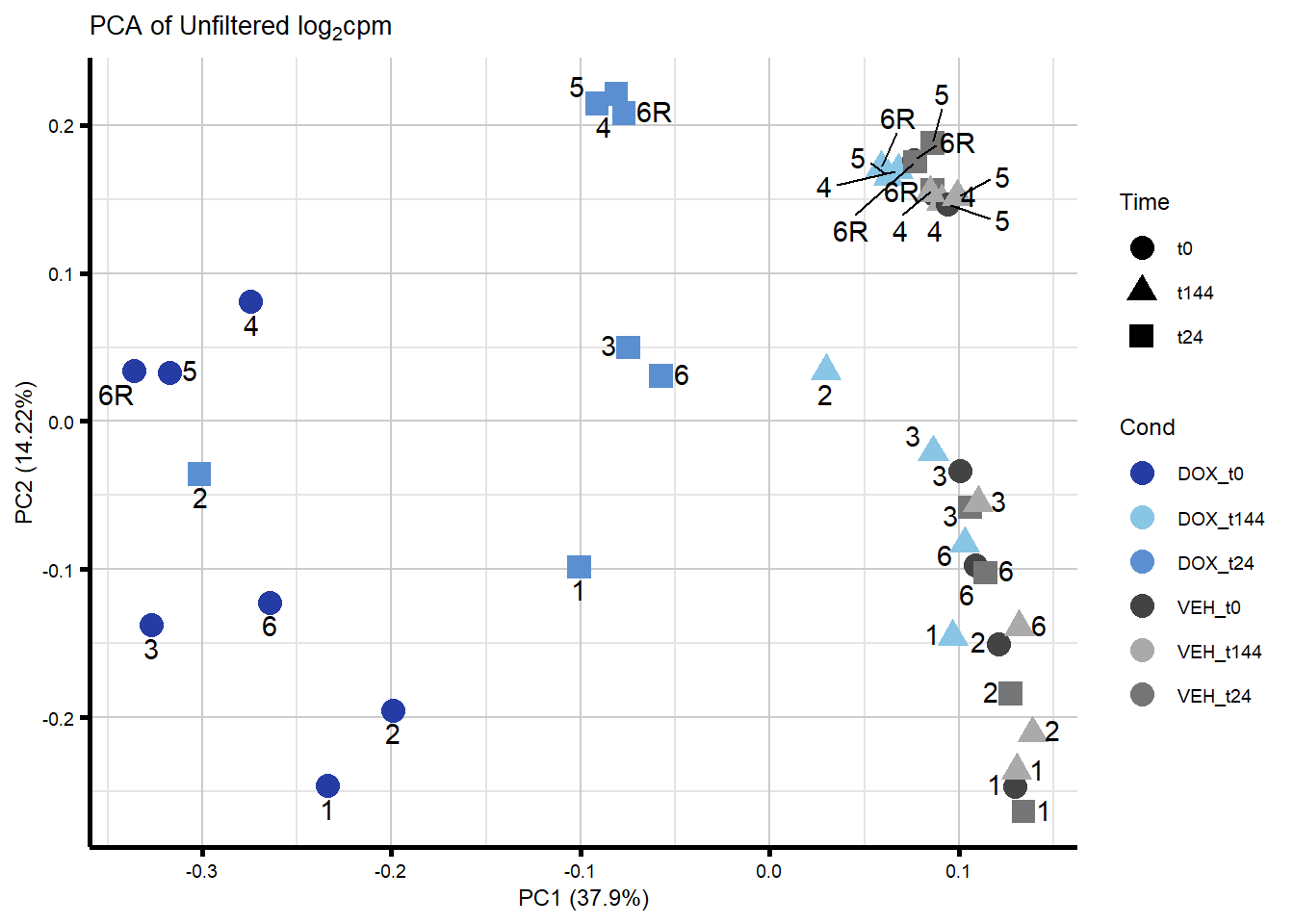
####PC2/PC3####
ggplot2::autoplot(prcomp_res_unfilt, data = Metadata, colour = "Cond"
                  , shape = "Time", size =4, x=2, y=3) +
  ggrepel::geom_text_repel(label=ind_num, vjust = -.5, max.overlaps = 30) +
  scale_color_manual(values=txtime_col) +
  ggtitle(expression("PCA of Unfiltered log"[2]*"cpm")) +
  theme_custom()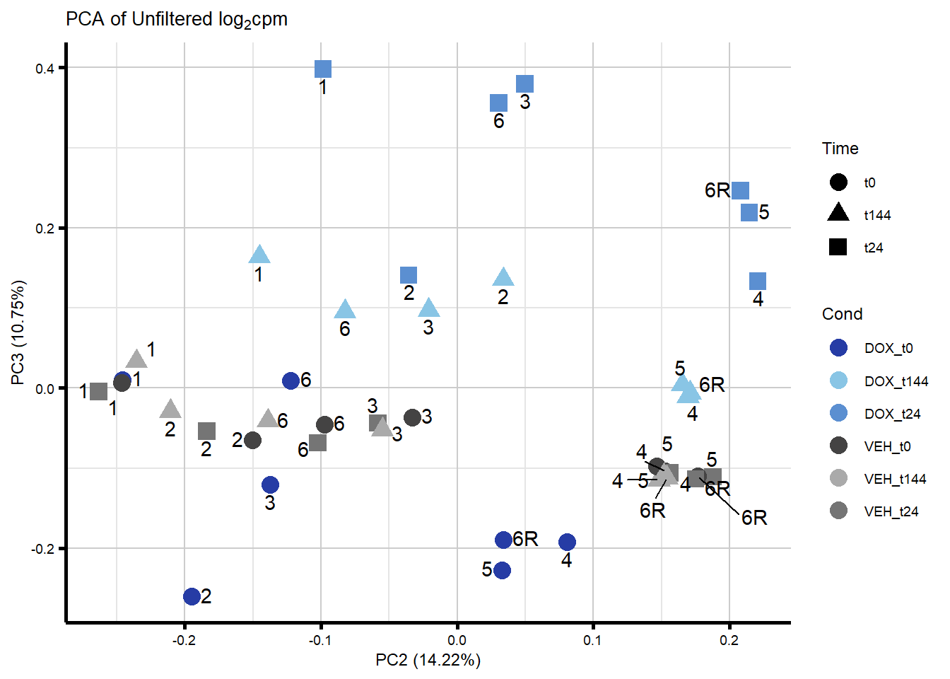
####PC3/PC4####
ggplot2::autoplot(prcomp_res_unfilt, data = Metadata, colour = "Cond", shape = "Time", size =4, x=3, y=4) +
  ggrepel::geom_text_repel(label=ind_num, vjust = -.5, max.overlaps = 30) +
  scale_color_manual(values=txtime_col) +
  ggtitle(expression("PCA of Unfiltered log"[2]*"cpm")) +
  theme_custom()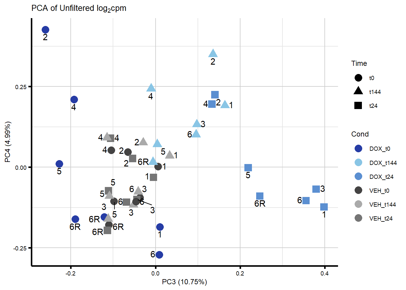
#Now plot my PCA for filtered log2cpm
####PC1/PC2####
ggplot2::autoplot(prcomp_res_filt, data = Metadata, colour = "Cond", shape = "Time", size =4, x=1, y=2) +
  ggrepel::geom_text_repel(label=ind_num, vjust = -.5, max.overlaps = 30) +
  scale_color_manual(values=txtime_col) +
  ggtitle(expression("PCA of Filtered log"[2]*"cpm")) +
  theme_custom()
ggplot2::autoplot(prcomp_res_filt, data = Metadata, colour = "Cond", shape = "Time", size =4, x=1, y=2) +
  ggrepel::geom_text_repel(label=ind_num, vjust = -.5, max.overlaps = 30) +
  scale_color_manual(values=txtime_col) +
  ggtitle(expression("PCA of Filtered log"[2]*"cpm")) +
  theme_custom()
####PC2/PC3####
ggplot2::autoplot(prcomp_res_filt, data = Metadata, colour = "Cond", shape = "Time", size =4, x=2, y=3) +
  ggrepel::geom_text_repel(label=ind_num, vjust = -.5, max.overlaps = 30) +
  scale_color_manual(values=txtime_col) +
  ggtitle(expression("PCA of Filtered log"[2]*"cpm")) +
  theme_custom()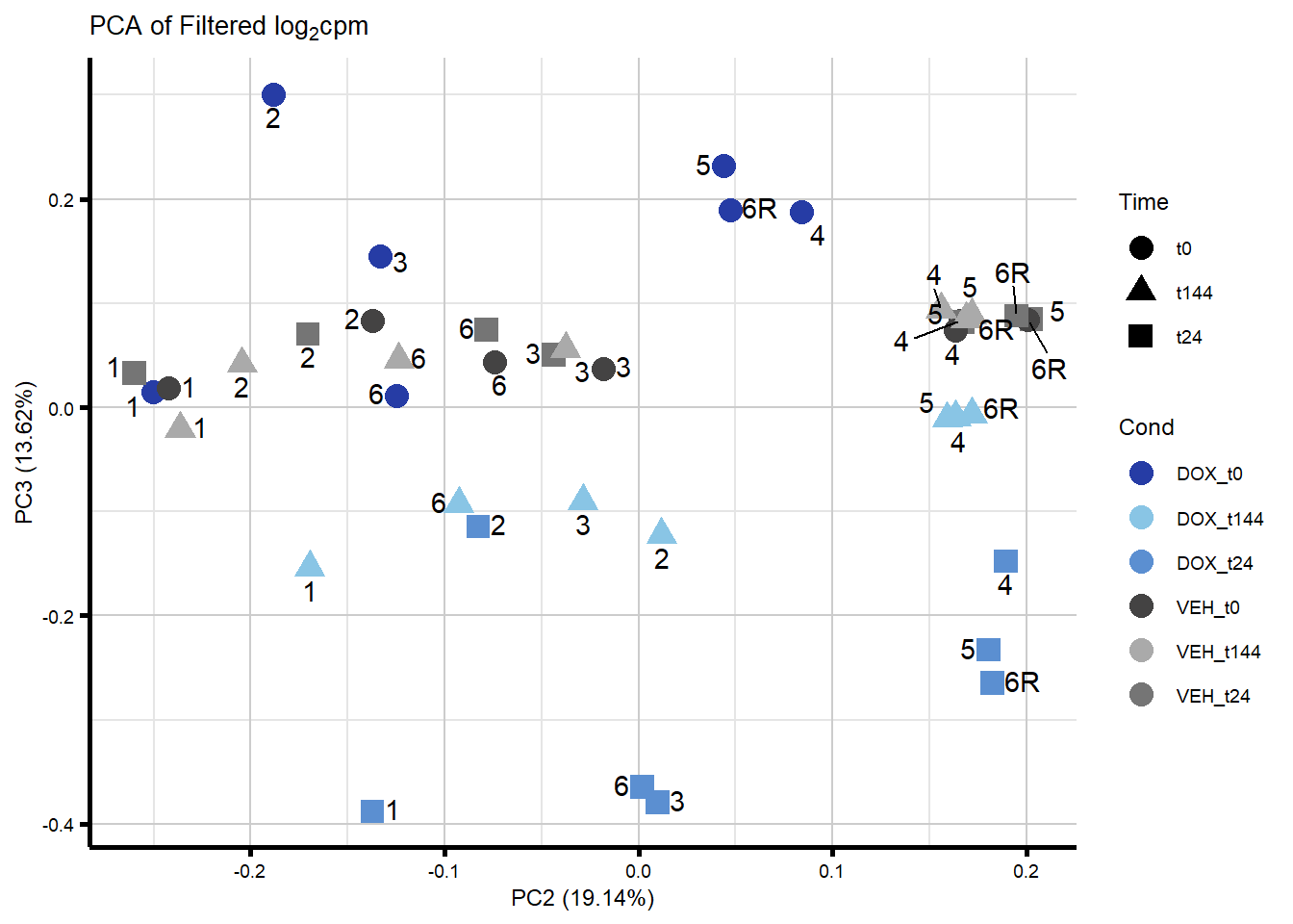
####PC3/PC4####
ggplot2::autoplot(prcomp_res_filt, data = Metadata, colour = "Cond", shape = "Time", size =4, x=3, y=4) +
  ggrepel::geom_text_repel(label=ind_num, vjust = -.5, max.overlaps = 30) +
  scale_color_manual(values=txtime_col) +
  ggtitle(expression("PCA of Filtered log"[2]*"cpm")) +
  theme_custom()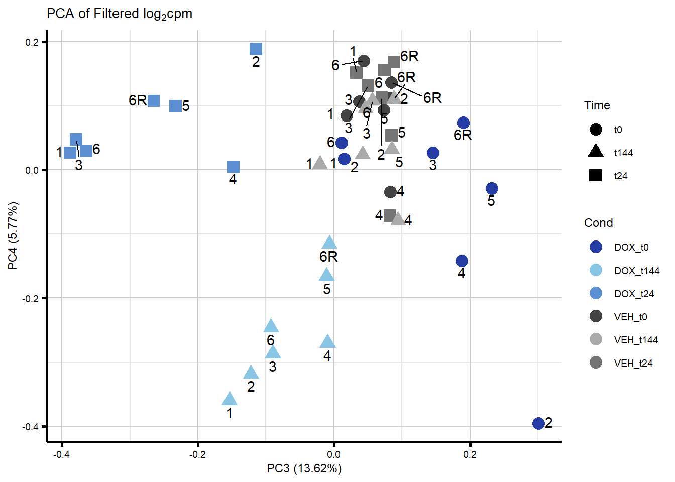
ggplot2::autoplot(prcomp_res_filt, data = Metadata, colour = "Cond", shape = "Time", size =4, x=1, y=2) +
  ggrepel::geom_text_repel(label=ind_num, vjust = -.5, max.overlaps = 30) +
  scale_color_manual(values=txtime_col) +
  ggtitle(expression("PCA of Filtered log"[2]*"cpm")) +
  theme_custom()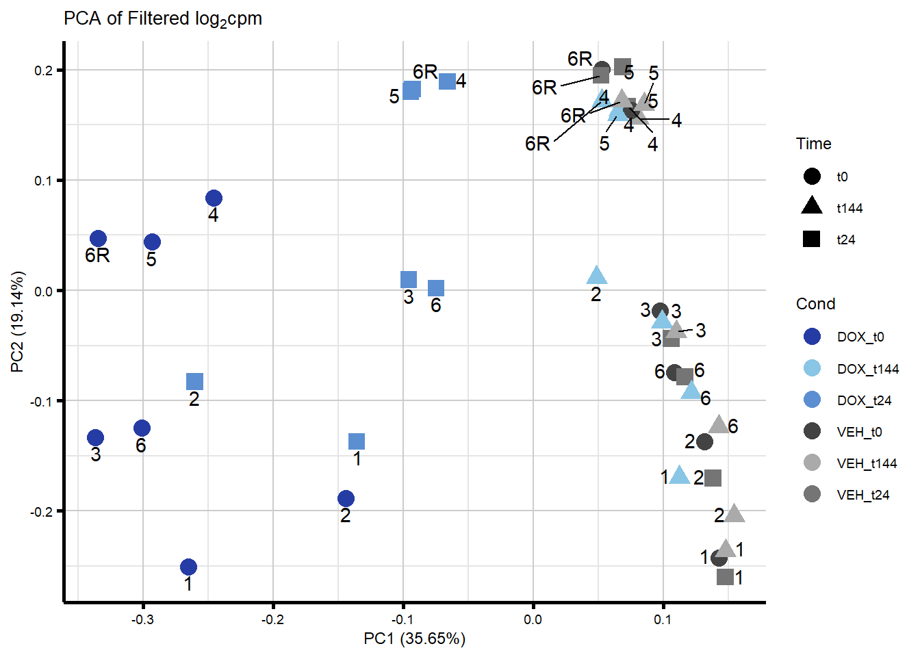
#now make a version for supplementary figure 2
autoplot(prcomp_res_filt,
         data = Metadata,
         colour = "Cond",
         shape = "Time",
         size = 5,
         x = 1,
         y = 2) +
  theme_custom() +
  scale_color_manual(values = txtime_col) +
  geom_text_repel(aes(label = ind_num),
                  nudge_y = 0.05,
                  max.overlaps = 50,
                  size = 5,
                  segment.color = "grey50") +
  ggtitle("PCA of global gene expression (pre-RUV)")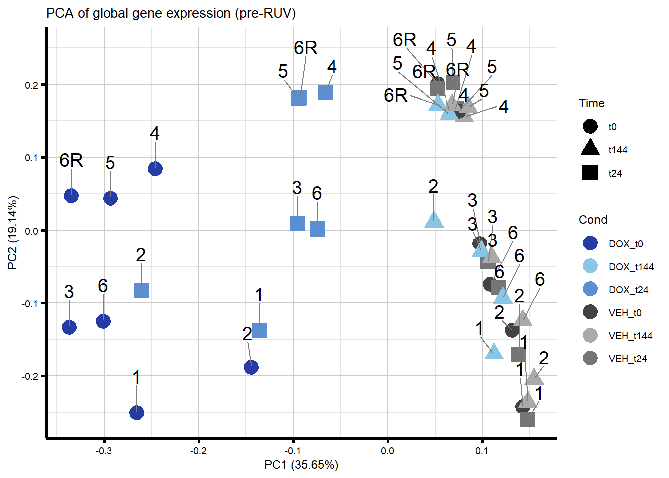
#save for figure generation

# ggsave("SuppFig2_pca_6x8_EMP.pdf", width = 8, height = 6, device = cairo_pdf,dpi = 300, path = output_folder)
Correlation Heatmaps
#check to make sure that the column names are correct
lcpm_2 <- filcpm_matrix
colnames(lcpm_2) <- Metadata$Final_sample_name

#compute the correlation matrices, one pearson and one spearman
cor_matrix_pearson <- cor(lcpm_2,
                          y = NULL,
                          use = "everything",
                          method = "pearson")
cor_matrix_spearman <- cor(lcpm_2,
                           y = NULL,
                           use = "everything",
                           method = "spearman")

# Extract metadata columns
Individual <- as.character(Metadata$Ind)
Time <- as.character(Metadata$Time)
Treatment <- as.character(Metadata$Treatment)

# Define color palettes for annotations
annot_col_cor = list(drugs = c("DOX" = "#499FBD",
                               "VEH" = "#BBBBBC"),
                     individuals = c("1" = "#FFA364",
                                     "2" = "#78EFDE",
                                     "3" = "#A4D177",
                                     "4" = "#EAD050",
                                     "5" = "#A68AC0",
                                     "6" = "#F16F90",
                                     "6R" = "#C61E4E"),
                     timepoints = c("t0" = "#005A4C",
                                    "t24" = "#328477",
                                    "t144" = "#8FB9B1"))

drug_colors <- c("DOX" = "#499FBD",
                 "VEH" = "#BBBBBC")
ind_colors <- c("1" = "#FFA364",
                "2" = "#78EFDE",
                "3" = "#A4D177",
                "4" = "#EAD050",
                "5" = "#A68AC0",
                "6" = "#F16F90",
                "6R" = "#C61E4E")
time_colors <- c("t0" = "#005A4C",
                 "t24" = "#328477",
                 "t144" = "#8FB9B1")

# Create annotations
top_annotation <- HeatmapAnnotation(
  Individual = Individual,
  Time = Time,
  Treatment = Treatment,
  col = list(
    Individual = ind_colors,
    Time = time_colors,
    Treatment = drug_colors
  )
)

####Pearson Heatmap####
heatmap_pearson <- Heatmap(cor_matrix_pearson,
                           name = "Pearson",
                           top_annotation = top_annotation,
                           show_row_names = TRUE,
                           show_column_names = TRUE,
                           cluster_rows = TRUE,
                           cluster_columns = TRUE,
                           border = TRUE)

# Draw the heatmap
draw(heatmap_pearson)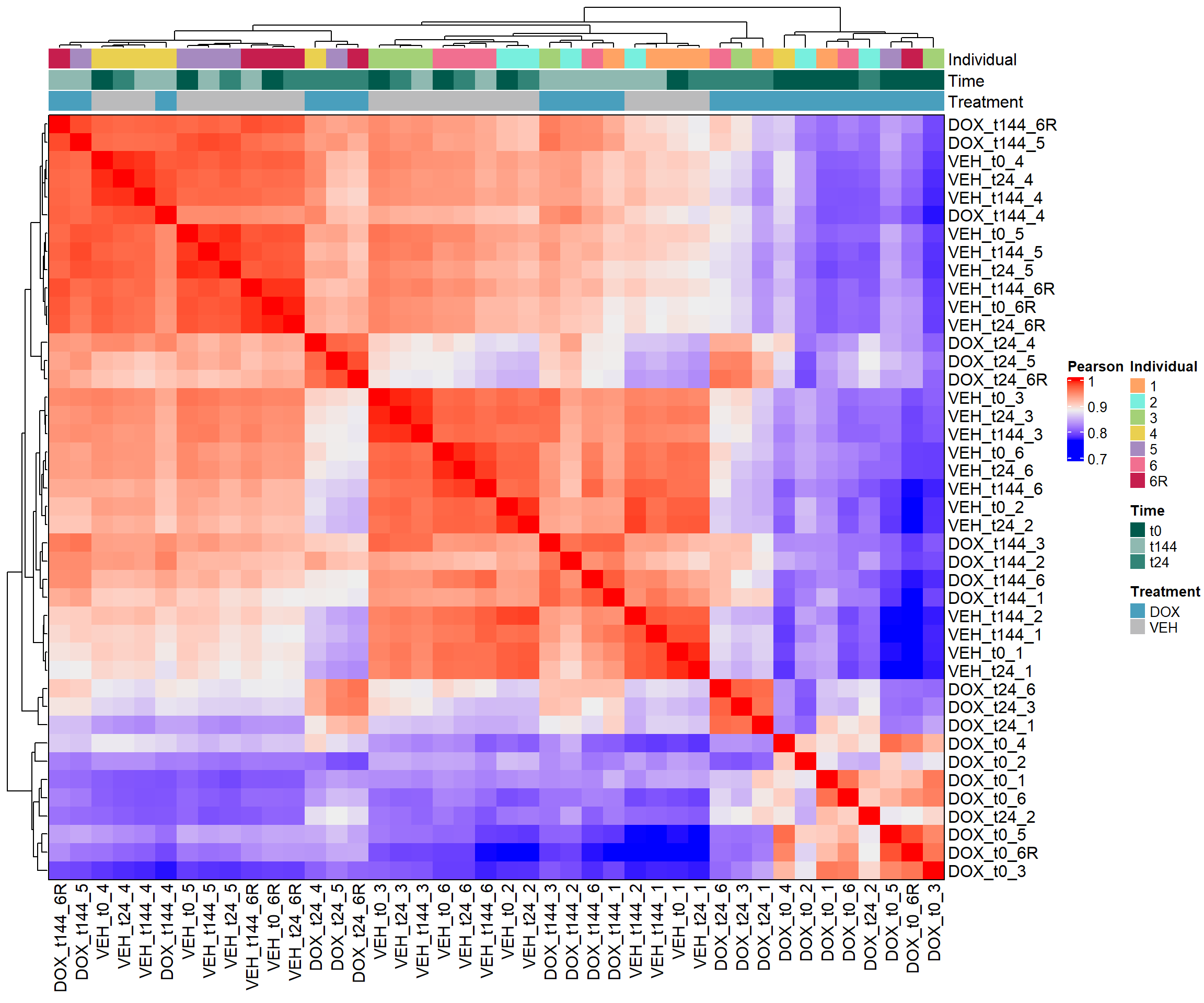
####Spearman Heatmap####
heatmap_spearman <- Heatmap(cor_matrix_spearman,
                           name = "Spearman",
                           top_annotation = top_annotation,
                           show_row_names = TRUE,
                           show_column_names = TRUE,
                           cluster_rows = TRUE,
                           cluster_columns = TRUE,
                           border = TRUE)

# Draw the heatmap
draw(heatmap_spearman)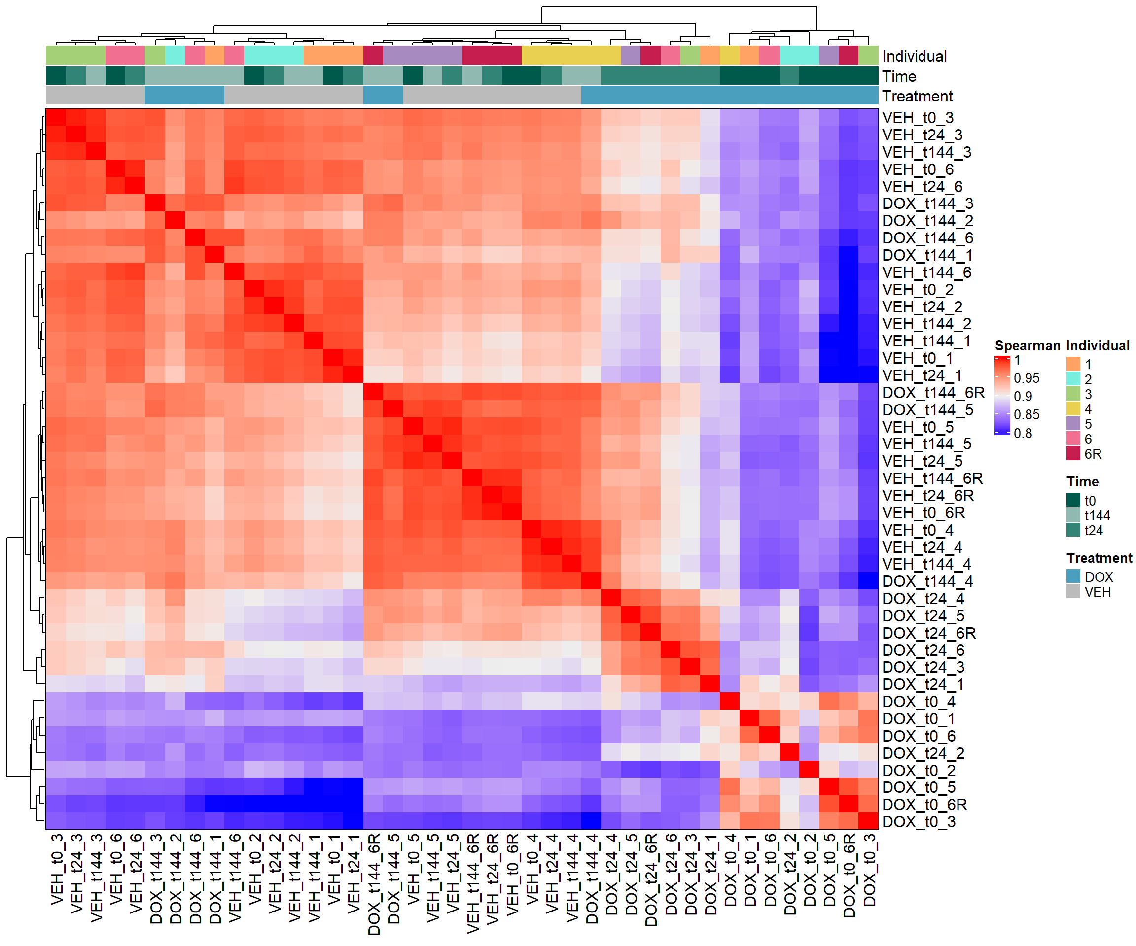
Filtered Gene List
#Now I want to make a filtered gene list (my rownames)
##I will use this to filter my counts for limma (+ Cormotif later on)

# filt_gene_list <- rownames(filcpm_matrix)
#save this filtered gene list as I'll use it to filter my counts
# saveRDS(filt_gene_list, "data/QC/filt_gene_list.RDS")

filt_gene_list <- readRDS("data/QC/filt_gene_list.RDS")
Filter Genes for Differential Expression Analysis
Perform preliminary DE analysis on non-corrected data to get a baseline for RUVs correction.
# counts_raw_matrix <- readRDS("data/QC/counts_raw_matrix.RDS")
#change column names to match samples for my raw counts matrix
#update them to the new nomenclature so I can have everything match up with Metadata new
# colnames(counts_raw_matrix) <- c("DOX_t0_1",
#                                 "VEH_t0_1",
#                                 "DOX_t24_1",
#                                 "VEH_t24_1",
#                                 "DOX_t144_1",
#                                 "VEH_t144_1",
#                                 "DOX_t0_2",
#                                 "VEH_t0_2",
#                                 "DOX_t24_2",
#                                 "VEH_t24_2",
#                                 "DOX_t144_2",
#                                 "VEH_t144_2",
#                                 "DOX_t0_3",
#                                 "VEH_t0_3",
#                                 "DOX_t24_3",
#                                 "VEH_t24_3",
#                                 "DOX_t144_3",
#                                 "VEH_t144_3",
#                                 "DOX_t0_4",
#                                 "VEH_t0_4",
#                                 "DOX_t24_4",
#                                 "VEH_t24_4",
#                                 "DOX_t144_4",
#                                 "VEH_t144_4",
#                                 "DOX_t0_5",
#                                 "VEH_t0_5",
#                                 "DOX_t24_5",
#                                 "VEH_t24_5",
#                                 "DOX_t144_5",
#                                 "VEH_t144_5",
#                                 "DOX_t0_6",
#                                 "VEH_t0_6",
#                                 "DOX_t24_6",
#                                 "VEH_t24_6",
#                                 "DOX_t144_6",
#                                 "VEH_t144_6",
#                                 "DOX_t0_6R",
#                                 "VEH_t0_6R",
#                                 "DOX_t24_6R",
#                                 "VEH_t24_6R",
#                                 "DOX_t144_6R",
#                                 "VEH_t144_6R")

# saveRDS(counts_raw_matrix, "data/QC/counts_raw_matrix.RDS")

counts_raw_matrix <- readRDS("data/QC/counts_raw_matrix.RDS")

#subset my count matrix based on filtered CPM matrix
x <- counts_raw_matrix[row.names(filcpm_matrix),]
dim(x)
[1] 14319 42# saveRDS(x, "data/DE/x_dge_counts_allind_updated.RDS")
#14319 genes as expected!
#this is still in counts form
#remove my replicate individual at this time
x_norep <- x[,1:36]
# saveRDS(x_norep, "data/DE/x_norep.RDS")
# Metadata <- read.csv("data/QC/Metadata_update.csv")
#
#modify my metadata to match
# Metadata_2 <- Metadata[1:36,]
# rownames(Metadata_2) <- Metadata_2$Sample_bam
# colnames(x_norep) <- Metadata_2$Sample_ID
# rownames(Metadata_2) <- Metadata_2$Sample_ID
# Metadata_2$Condition <- make.names(Metadata_2$Cond)
# Metadata_2$Ind <- as.character(Metadata_2$Ind)
# saveRDS(Metadata_2, "data/QC/Metadata_2_norep_update.RDS")
Metadata_2 <- readRDS("data/QC/Metadata_2_norep_update.RDS")Perform DE Analysis
#create DGEList object
dge <- DGEList(counts = x_norep)
dge$samples$group <- factor(Metadata_2$Condition)
dge <- calcNormFactors(dge, method = "TMM")

# saveRDS(dge, "data/DE/dge_matrix.RDS")

# check normalization factors from TMM normalization of LIBRARIES
dge$samples
group lib.size norm.factors
DOX_t0_1 DOX_t0 19935097 1.0526605
VEH_t0_1 VEH_t0 21302879 0.9773889
DOX_t24_1 DOX_t24 25636959 1.0751043
VEH_t24_1 VEH_t24 26319662 0.9940323
DOX_t144_1 DOX_t144 23463426 0.9003102
VEH_t144_1 VEH_t144 25840938 0.9888449
DOX_t0_2 DOX_t0 23085807 0.7676077
VEH_t0_2 VEH_t0 25610495 1.0077383
DOX_t24_2 DOX_t24 18083930 1.1682704
VEH_t24_2 VEH_t24 24331177 0.9906872
DOX_t144_2 DOX_t144 19754391 0.9941834
VEH_t144_2 VEH_t144 22641509 1.0010734
DOX_t0_3 DOX_t0 20583626 1.0676786
VEH_t0_3 VEH_t0 28166198 1.0031906
DOX_t24_3 DOX_t24 25831427 1.1530208
VEH_t24_3 VEH_t24 26081158 1.0058953
DOX_t144_3 DOX_t144 24659898 0.9261599
VEH_t144_3 VEH_t144 25412931 0.9703454
DOX_t0_4 DOX_t0 23393931 0.9745263
VEH_t0_4 VEH_t0 22853195 0.9565797
DOX_t24_4 DOX_t24 23846995 1.1659432
VEH_t24_4 VEH_t24 21299355 0.9649641
DOX_t144_4 DOX_t144 18222568 0.9913625
VEH_t144_4 VEH_t144 28115884 0.9653464
DOX_t0_5 DOX_t0 22518848 0.9766893
VEH_t0_5 VEH_t0 24589534 0.9612345
DOX_t24_5 DOX_t24 24797547 1.1703079
VEH_t24_5 VEH_t24 25977536 0.9509690
DOX_t144_5 DOX_t144 27447106 0.9422729
VEH_t144_5 VEH_t144 24893583 0.9356377
DOX_t0_6 DOX_t0 25187428 1.0311957
VEH_t0_6 VEH_t0 25630519 1.0283437
DOX_t24_6 DOX_t24 26138399 1.1183471
VEH_t24_6 VEH_t24 24430396 0.9988688
DOX_t144_6 DOX_t144 23323463 0.9496884
VEH_t144_6 VEH_t144 25424152 0.9872926#create my design matrix for DE
design <- model.matrix(~ 0 + Metadata_2$Condition)
colnames(design) <- gsub("Metadata_2\\$Condition", "", colnames(design))
#take care that the matrix automatically sorts cols alphabetically
##currently DOX_t0, DOX_t144, DOX_t24, VEH_t0, VEH_t144, VEH_t24
#run duplicate correlation for individual effect
corfit <- duplicateCorrelation(object = dge$counts, design = design, block = Metadata_2$Ind)
#voom transformation and plot
v <- voom(dge, design, block = Metadata_2$Ind, correlation = corfit$consensus.correlation, plot = TRUE)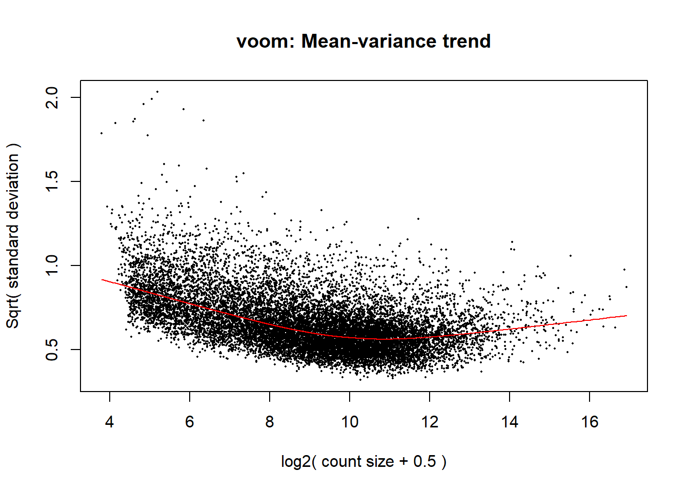
#fit my linear model
fit <- lmFit(v, design, block = Metadata_2$Ind, correlation = corfit$consensus.correlation)

#make my contrast matrix to compare across tx and veh
contrast_matrix <- makeContrasts(
  V.D24T = DOX_t0 - VEH_t0,
  V.D24R = DOX_t24 - VEH_t24,
  V.D144R = DOX_t144 - VEH_t144,
  levels = design
)

#apply these contrasts to compare DOX to DMSO VEH
fit2 <- contrasts.fit(fit, contrast_matrix)
fit2 <- eBayes(fit2)

#plot the mean-variance trend
plotSA(fit2, main = "Final model: Mean-Variance trend")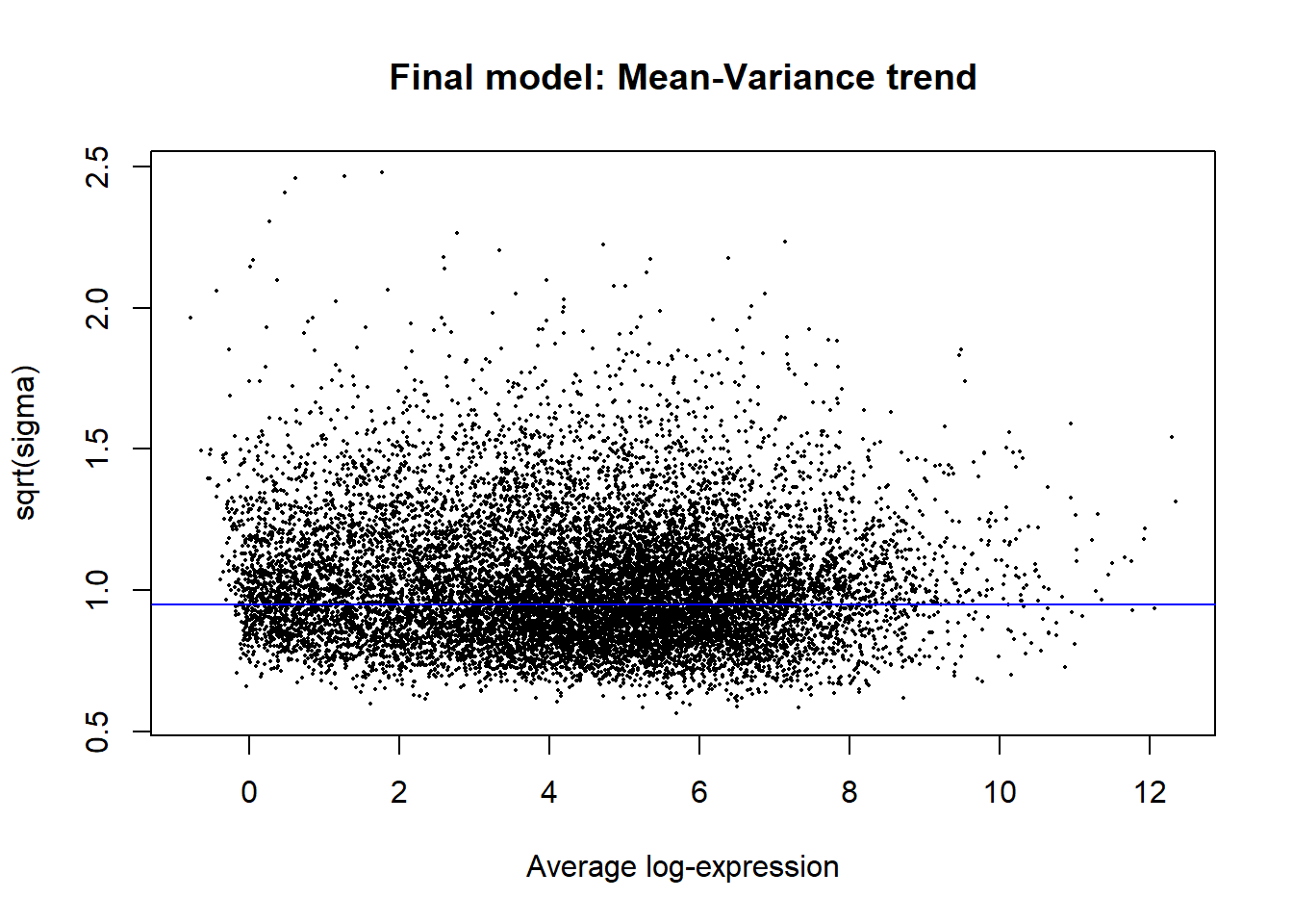
#look at the summary of your results
##this tells you the number of DEGs in each condition
results_summary <- decideTests(fit2, adjust.method = "BH", p.value = 0.05)
summary(results_summary)
V.D24T V.D24R V.D144R
Down 4723 3593 359
NotSig 5076 7151 13810
Up 4520 3575 150# V.D24 V.D24r V.D144r
# Down 4723 3593 359
# NotSig 5076 7151 13810
# Up 4520 3575 150Create Prelim Toptables
These toptables will not be used later as they need to be corrected, but let’s look at what the data looks like before RUVs correction.
# Generate Top Table for Specific Comparisons

Toptable_V.D24T <- topTable(fit = fit2, coef = "V.D24T", number = nrow(x), adjust.method = "BH", p.value = 1, sort.by = "none")
# write.csv(Toptable_V.D24T, "data/DE/Toptable_V.D24T_noRUV.csv")

Toptable_V.D24R <- topTable(fit = fit2, coef = "V.D24R", number = nrow(x), adjust.method = "BH", p.value = 1, sort.by = "none")
# write.csv(Toptable_V.D24R, "data/DE/Toptable_V.D24R_noRUV.csv")

Toptable_V.D144R <- topTable(fit = fit2, coef = "V.D144R", number = nrow(x), adjust.method = "BH", p.value = 1, sort.by = "none")
# write.csv(Toptable_V.D144R, "data/DE/Toptable_V.D144R_noRUV.csv")

#save all of these toptables as R objects
# saveRDS(list(
#   V.D24T = Toptable_V.D24T,
#   V.D24R = Toptable_V.D24R,
#   V.D144R = Toptable_V.D144R
# ), file = "data/DE/Toptable_list_noRUV.RDS")

Toptable_list_noRUV <- readRDS("data/DE/Toptable_list_noRUV.RDS")
logFC Boxplots of DE by Timepoint
# Load DEGs Data
DOX_24T <- read.csv("data/DE/Toptable_V.D24T_noRUV.csv", row.names = 1)
DOX_24R <- read.csv("data/DE/Toptable_V.D24R_noRUV.csv", row.names = 1)
DOX_144R <- read.csv("data/DE/Toptable_V.D144R_noRUV.csv", row.names = 1)

#make a list of all of the genes in this set so I can plot the logFC in other sets
D24T_DEGs <- rownames(DOX_24T)[DOX_24T$adj.P.Val < 0.05]
length(D24T_DEGs)
[1] 9243#9243 genes in length after adj. p value cutoff
#now that I have a list of my DEGs from D24T - pull these genes out from the other DEG lists
D24R_DEGs <- rownames(DOX_24R)[DOX_24R$adj.P.Val < 0.05]
length(D24R_DEGs)[1] 7168#7168 genes here
D144R_DEGs <- rownames(DOX_144R)[DOX_144R$adj.P.Val < 0.05]
length(D144R_DEGs)[1] 509#509 genes in 144R
#Combine the toptables I have from pairwise analysis into a single dataframe
d0_toptable_dxr <- Toptable_V.D24T %>%
rownames_to_column(var = "Entrez_ID") %>%
mutate(Time = "t0")
d24_toptable_dxr <- Toptable_V.D24R %>%
rownames_to_column(var = "Entrez_ID") %>%
mutate(Time = "t24")
d144_toptable_dxr <- Toptable_V.D144R %>%
rownames_to_column(var = "Entrez_ID") %>%
mutate(Time = "t144")
combined_toptables_dxr <- bind_rows(
d0_toptable_dxr,
d24_toptable_dxr,
d144_toptable_dxr)
# saveRDS(combined_toptables_dxr, "data/DE/combined_toptables_dxr.RDS")
#Filter the data based on each timepoint
filt_toptable_dxr_t0 <- combined_toptables_dxr %>%
dplyr::filter(Entrez_ID %in% D24T_DEGs) %>%
mutate(absFC = abs(logFC)) %>%
mutate(time = factor(Time, levels = c("t0", "t24", "t144"), labels = c("t0", "t24", "t144"))) %>%
ggplot(., aes(x = time, y = logFC)) +
geom_boxplot(aes(fill = time)) +
scale_fill_manual(values = time_col) +
guides(fill = guide_legend(title = "Time")) +
xlab(" ") +
ylab("logFC") +
theme_custom() +
ggtitle("LogFC for t0 DEGs Across Conditions")
filt_toptable_dxr_t24 <- combined_toptables_dxr %>%
dplyr::filter(Entrez_ID %in% D24R_DEGs) %>%
mutate(absFC = abs(logFC)) %>%
mutate(time = factor(Time, levels = c("t0", "t24", "t144"), labels = c("t0", "t24", "t144"))) %>%
ggplot(., aes(x = time, y = logFC)) +
geom_boxplot(aes(fill = time)) +
scale_fill_manual(values = time_col) +
guides(fill = guide_legend(title = "Time")) +
theme_custom() +
xlab(" ") +
ylab("logFC") +
theme_custom() +
ggtitle("LogFC for t24 DEGs Across Conditions")
#D144R
filt_toptable_dxr_t144 <- combined_toptables_dxr %>%
dplyr::filter(Entrez_ID %in% D144R_DEGs) %>%
mutate(absFC = abs(logFC)) %>%
mutate(time = factor(Time, levels = c("t0", "t24", "t144"), labels = c("t0", "t24", "t144"))) %>%
ggplot(., aes(x = time, y = logFC))+
geom_boxplot(aes(fill = time))+
scale_fill_manual(values = time_col)+
guides(fill = guide_legend(title = "Time"))+
theme_custom()+
xlab(" ")+
ylab("logFC")+
theme_custom()+
ggtitle("LogFC for t144 DEGs Across Conditions")
#now put the names of these graphs to print them
filt_toptable_dxr_t0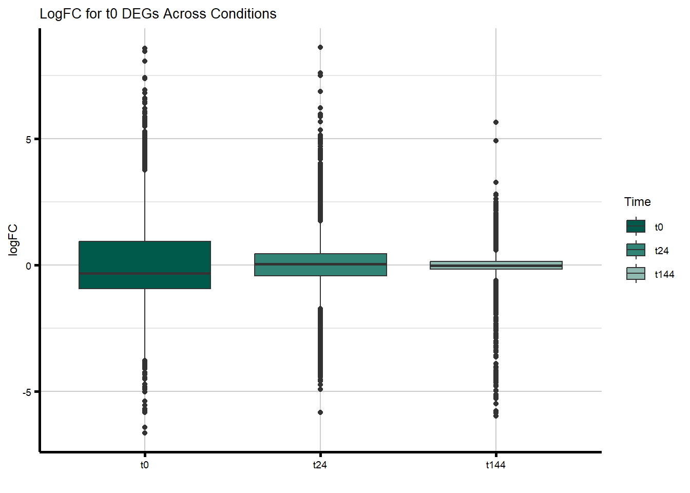
filt_toptable_dxr_t24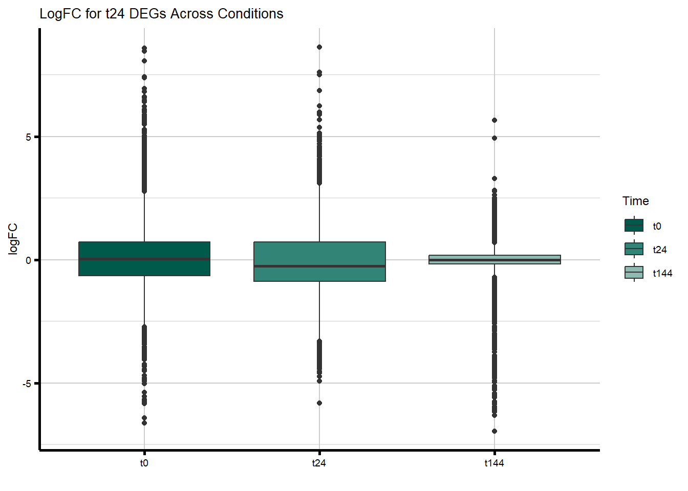
filt_toptable_dxr_t144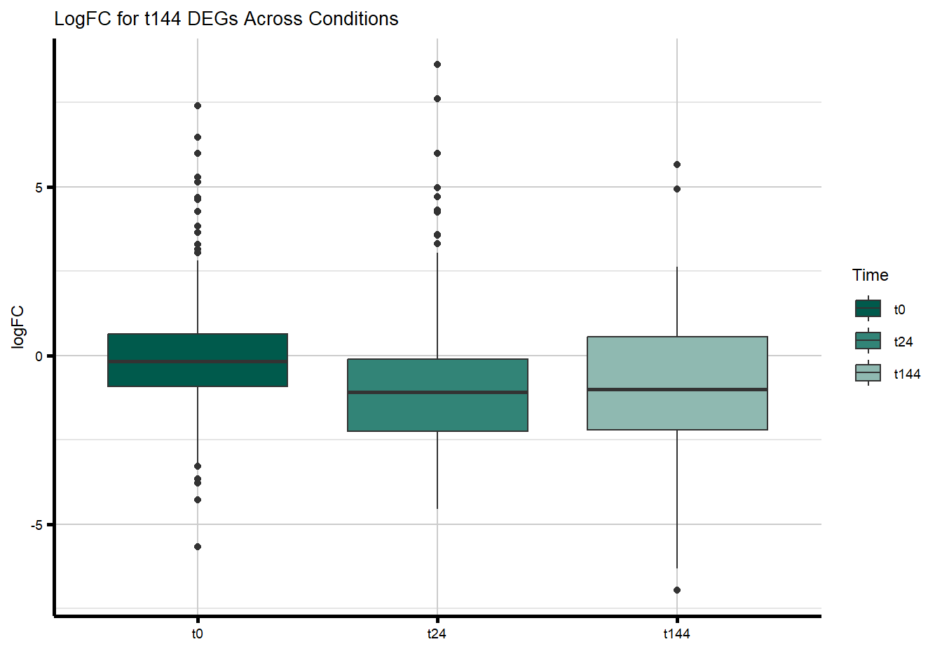
RUVs Correction
Correct for unwanted variation using RUVs, which uses a set of replicates to correct for variation.
Set Up Data Workflow
filt_gene_list <- rownames(filcpm_matrix)
#14319 genes as usual

#in order to make this match with annot later down the line, change the col names for counts_raw_matrix to match final_sample_names in annot

#i'll also want to make sure I keep the replicate for this set

colnames(counts_raw_matrix) <- Metadata$Final_sample_name

RUV_filt_counts <- counts_raw_matrix %>%
  as.data.frame() %>%
  dplyr::filter(., row.names(.)%in% filt_gene_list)
# saveRDS(RUV_filt_counts, "data/DE/RUV_filt_counts.RDS")

#add in the annotation files
ind_num <- readRDS("data/QC/ind_num.RDS")
annot <- read.csv("data/QC/Metadata_update.csv")
#same as Metadata


#  counts need to be integer values and in a numeric matrix
# note: the log transformation needs to be accounted for in the isLog argument in RUVs function.
counts <- as.matrix(RUV_filt_counts)

# saveRDS(counts, "data/new/RUV/filt_counts_matrix.RDS")

# Create a DataFrame for the phenoData
phenoData <- DataFrame(annot)

# Now create the RangedSummarizedExperiment necessary for RUVs input
# looks like it did need both the phenodata and the counts.
set <- SummarizedExperiment(assays =  counts, metadata = phenoData)

# Generate a background matrix
# The column "Cond" holds the comparisons that you actually want to make. DOX_24, DMSO_24,5FU_24, DOX_3,etc.
scIdx <- RUVSeq::makeGroups(phenoData$Cond)
scIdx
[,1] [,2] [,3] [,4] [,5] [,6] [,7]
[1,] 1 7 13 19 25 31 37
[2,] 5 11 17 23 29 35 41
[3,] 3 9 15 21 27 33 39
[4,] 2 8 14 20 26 32 38
[5,] 6 12 18 24 30 36 42
[6,] 4 10 16 22 28 34 40#now I've made all of the data I need for this - they are located in each section for k values
#DO NOT USE THESE COUNTS FOR LINEAR MODELING
#colors for all of the plots
# txtime_col
# ind_col
# time_col
# tx_col
# before ruv (counts PCA)
prcomp_res_counts <- prcomp(t(counts), scale. = FALSE, center = TRUE)
annot_prcomp_res <- prcomp_res_counts$x %>% cbind(., annot)
group_2 <- annot$Cond
#now plot my PCA for filtered counts
####PC1/PC2####
ggplot2::autoplot(prcomp_res_counts,
data = annot,
colour = "Cond",
shape = "Time",
size = 4,
x = 1,
y = 2) +
ggrepel::geom_text_repel(label = ind_num,
vjust = -0.5,
max.overlaps = 30) +
scale_color_manual(values = txtime_col) +
ggtitle(expression("PCA of Filtered Counts")) +
theme_custom()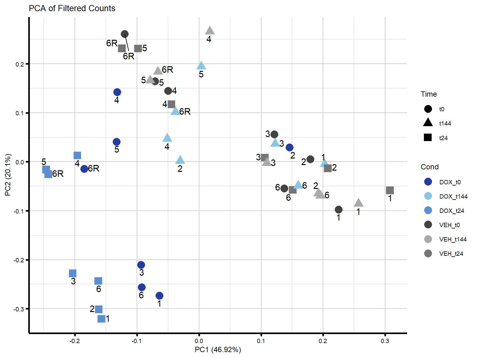
####PC2/PC3####
ggplot2::autoplot(prcomp_res_counts,
                  data = annot,
                  colour = "Cond",
                  shape = "Time",
                  size = 4,
                  x = 2,
                  y = 3) +
  ggrepel::geom_text_repel(label = ind_num,
                           vjust = -0.5,
                           max.overlaps = 30) +
  scale_color_manual(values = txtime_col) +
  ggtitle(expression("PCA of Filtered Counts")) +
  theme_custom()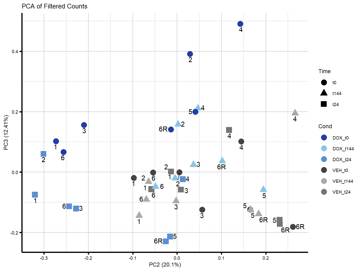
#go ahead and plot PCA of log2cpm to compare (somewhat) later since the norm counts output isn't possible with these data since they don't undergo correction

prcomp_res_cpm <- prcomp(t(filcpm_matrix %>% as.matrix()), center =  TRUE)

####PC1/PC2####
ggplot2::autoplot(prcomp_res_cpm,
                  data = annot,
                  colour = "Cond",
                  shape = "Time",
                  size = 4,
                  x = 1,
                  y = 2) +
  ggrepel::geom_text_repel(label = ind_num,
                           vjust = -0.5,
                           max.overlaps = 30) +
  scale_color_manual(values = txtime_col) +
  ggtitle(expression("PCA of log2cpm no RUVs")) +
  theme_custom()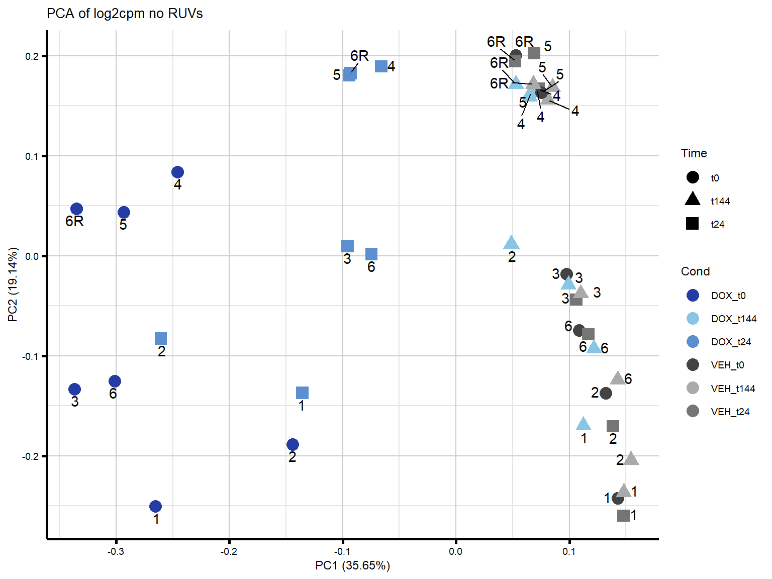
####PC2/PC3####
ggplot2::autoplot(prcomp_res_cpm,
                  data = annot,
                  colour = "Cond",
                  shape = "Time",
                  size = 4,
                  x = 2,
                  y = 3) +
  ggrepel::geom_text_repel(label = ind_num,
                           vjust = -0.5,
                           max.overlaps = 30) +
  scale_color_manual(values = txtime_col) +
  ggtitle(expression("PCA of log2cpm no RUVs")) +
  theme_custom()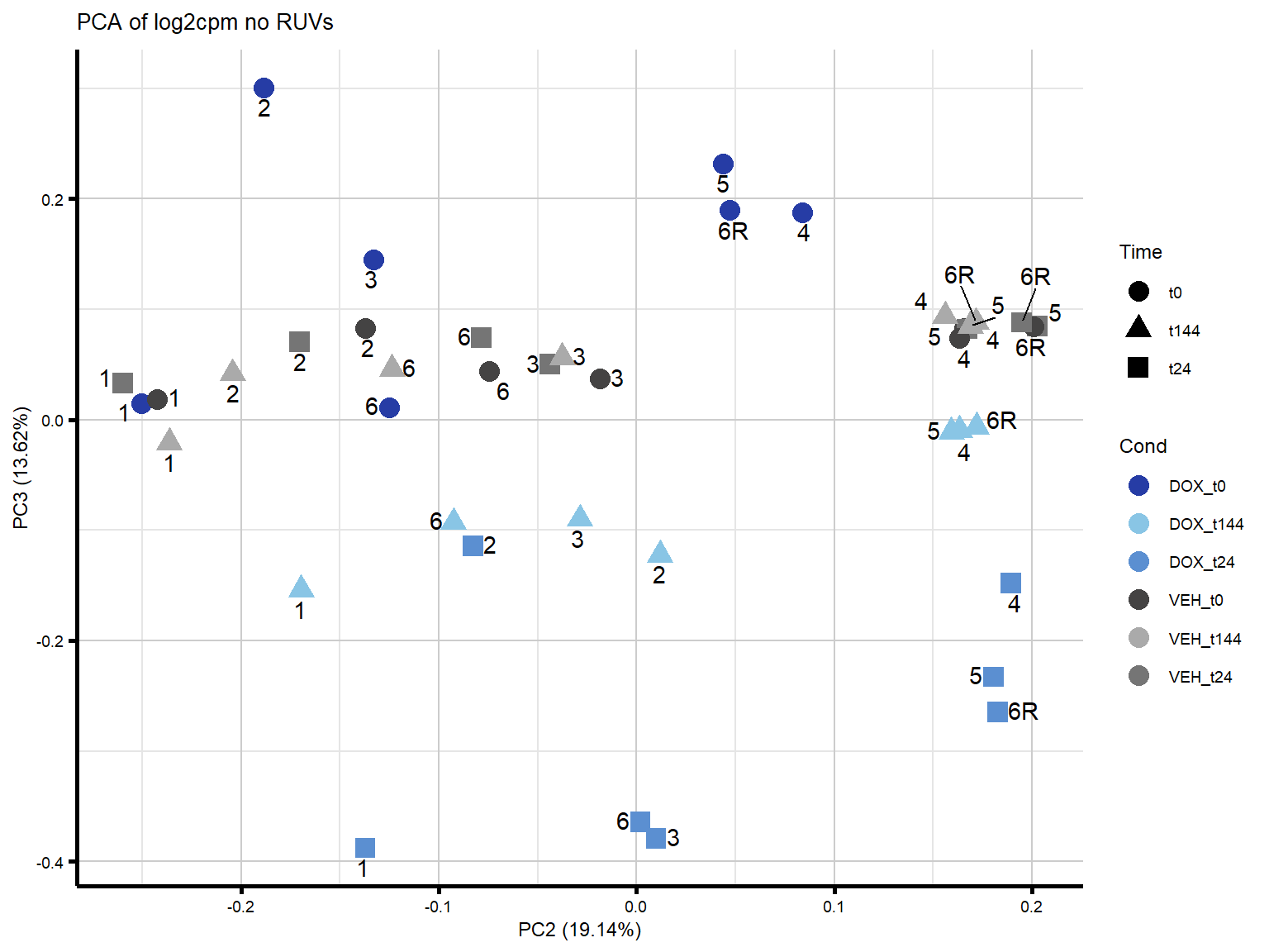
RUVs k=1, 1 factor of unwanted variation
#Apply RUVs function from RUVSeq
#"k" can be iteratively adjusted over time depending on PCA.
set1 <- RUVSeq::RUVs(x = counts, k =1, scIdx = scIdx, isLog = FALSE)
# saveRDS(set1, "data/DE/set1.RDS")
#get the ruv weights to put into the linear model. n weights = k.
#k=1
RUV_df1 <- set1$W %>% as.data.frame()
RUV_df1$Names <- rownames(RUV_df1)

#Check that the names match
#k=1
RUV_df_rm1 <- RUV_df1[RUV_df1$Names %in% annot$Final_sample_name, ]
RUV_1 <-  RUV_df_rm1$W_1

# saveRDS(RUV_df_rm1, "data/DE/RUV_df_rm1.RDS")
# saveRDS(RUV_1, "data/DE/RUV_1.RDS")

#PCA checks
#k=1
prcomp_res_1 <- prcomp(t(set1$normalizedCounts), scale. = FALSE, center = TRUE)
annot_prcomp_res_1 <- prcomp_res_1$x %>% cbind(., annot)

ggplot2::autoplot(prcomp_res_1,
                  data = annot,
                  colour = "Cond",
                  shape = "Time",
                  size =4,
                  x = 1,
                  y = 2)+
  theme_custom()+
  scale_color_manual(values = txtime_col)+
  ggrepel::geom_text_repel(label = ind_num,
                           vjust = -0.5,
                           max.overlaps = 30)+
  ggtitle("RUVs Correction k=1 NormCounts")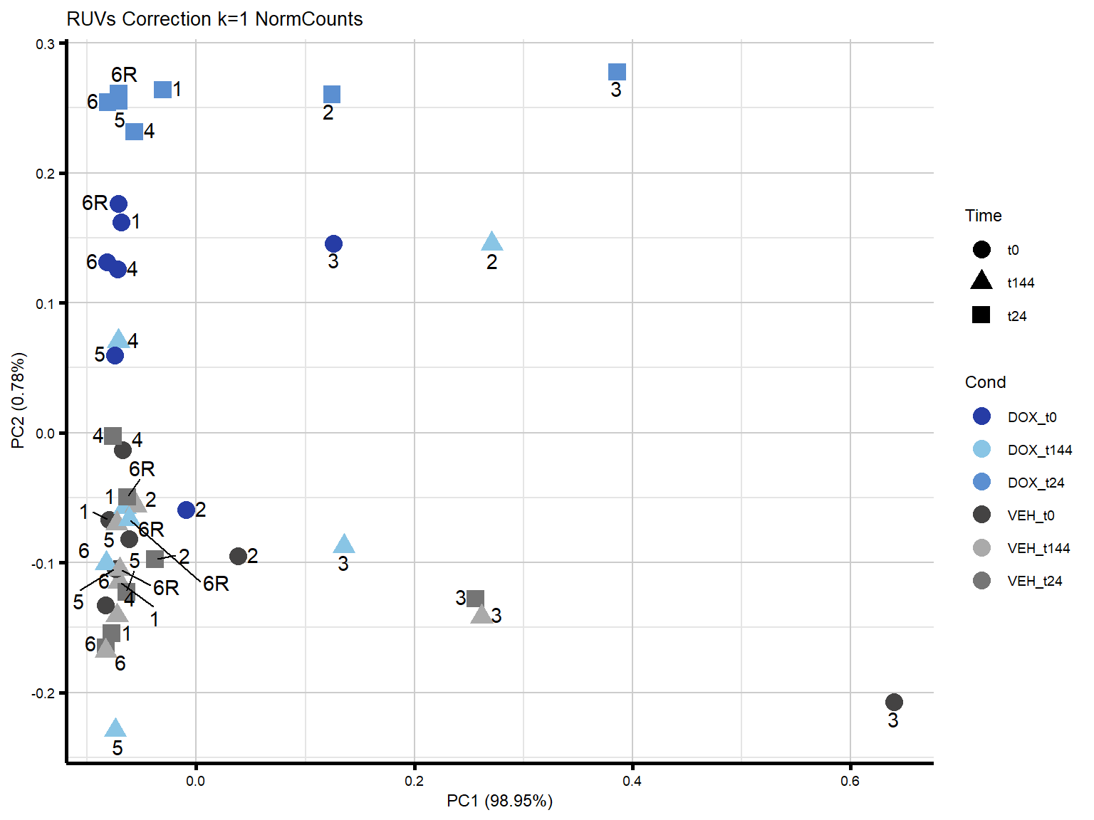
ggplot2::autoplot(prcomp_res_1,
                  data = annot,
                  colour = "Cond",
                  shape = "Time",
                  size = 4,
                  x = 2,
                  y = 3)+
  theme_custom()+
  scale_color_manual(values = txtime_col)+
  ggrepel::geom_text_repel(label = ind_num,
                           vjust = -0.5,
                           max.overlaps = 30)+
  ggtitle("RUVs Correction k=1 NormCounts")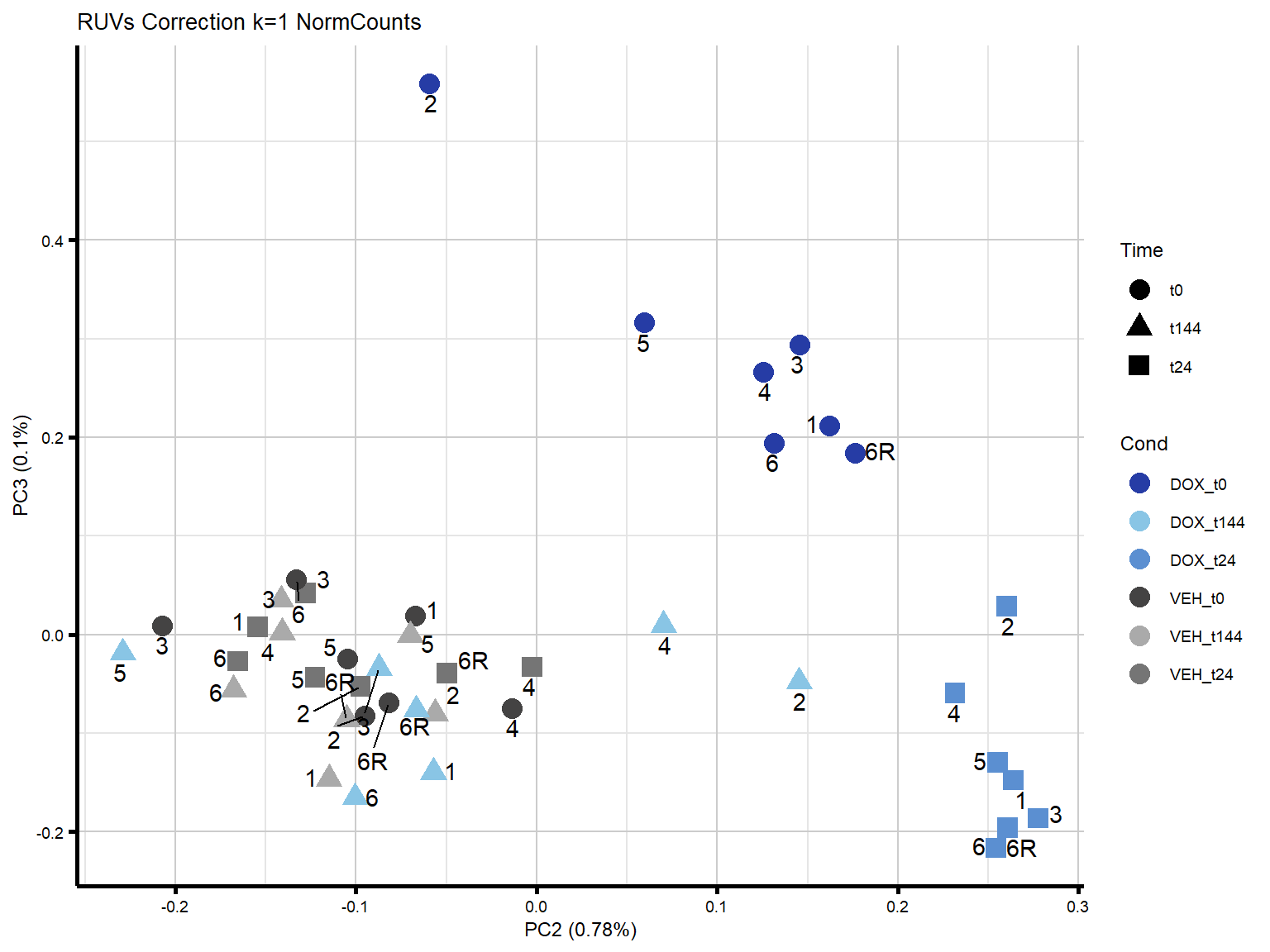
#also try by converting these values to log2cpm

RUV_df_rm1_cpm <- cpm(set1$normalizedCounts, log = TRUE)

prcomp_res_1_cpm <- prcomp(t(RUV_df_rm1_cpm), scale. = FALSE, center = TRUE)
annot_prcomp_res_1_cpm <- prcomp_res_1_cpm$x %>% cbind(., annot)

##PC1/2
ggplot2::autoplot(prcomp_res_1_cpm,
                  data = annot,
                  colour = "Cond",
                  shape = "Time",
                  size = 4,
                  x = 1,
                  y = 2)+
  theme_custom()+
  scale_color_manual(values = txtime_col)+
  ggrepel::geom_text_repel(label = ind_num,
                           vjust = -0.5,
                           max.overlaps = 50)+
  ggtitle("RUVs Correction k=1 log2cpm")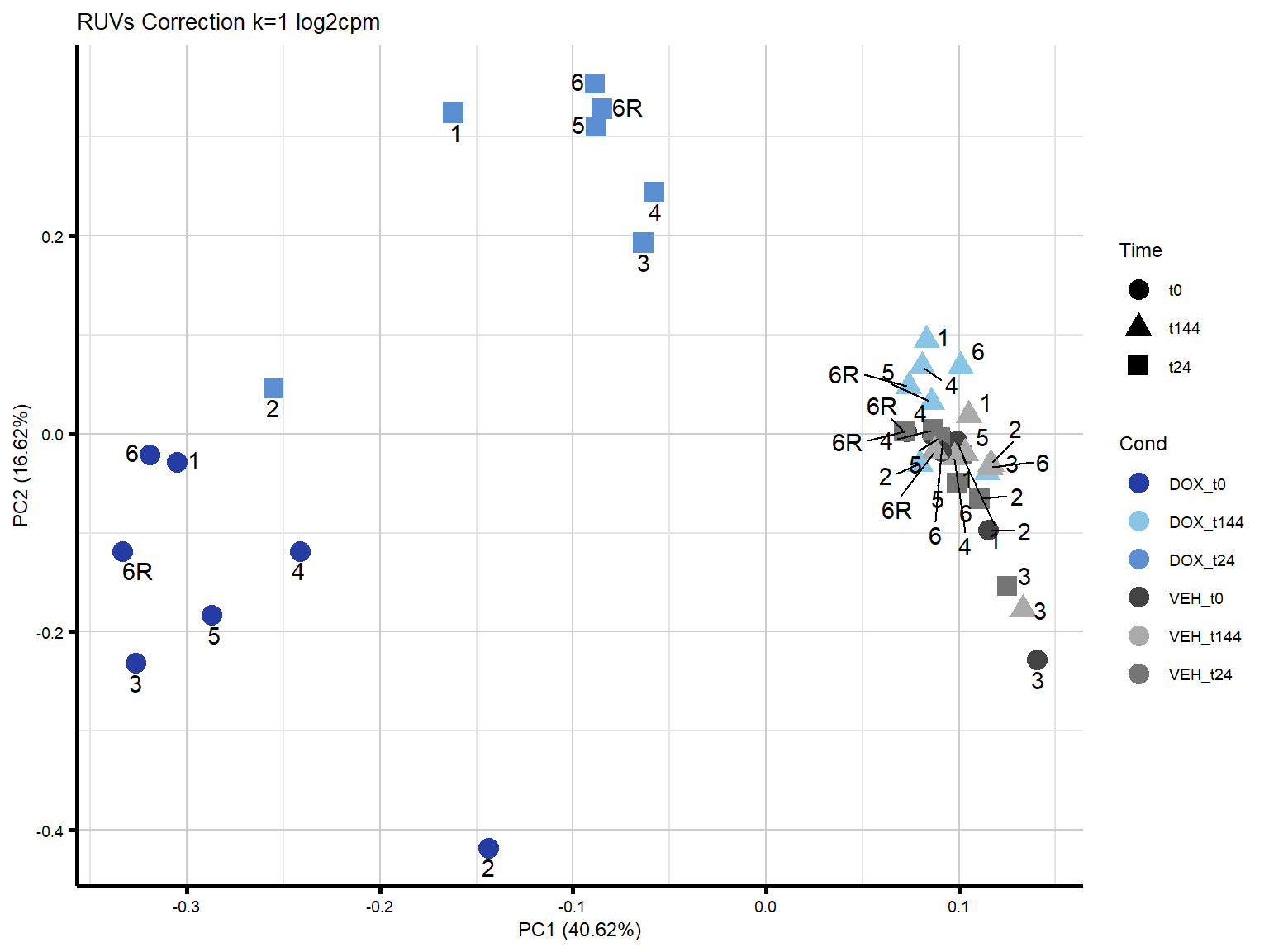
###PC2/3
ggplot2::autoplot(prcomp_res_1_cpm,
                  data = annot,
                  colour = "Cond",
                  shape = "Time",
                  size = 4,
                  x = 2,
                  y = 3)+
  theme_custom()+
  scale_color_manual(values = txtime_col)+
  ggrepel::geom_text_repel(label = ind_num,
                           vjust = -0.5,
                           max.overlaps = 30)+
  ggtitle("RUVs Correction k=1 log2cpm")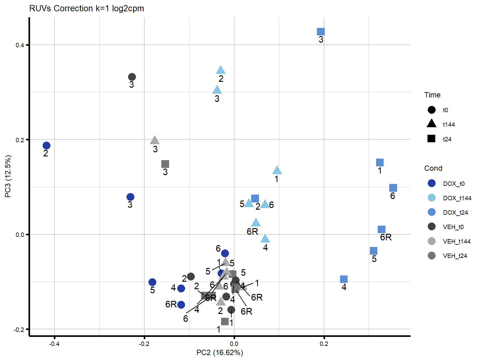
Spearman Correlation Heatmaps RUVs
#Now that I've put together the PCA plots for both normalized counts and log2cpm
#I want to make these into heatmaps

#first change your Metadata to have the new names for my supp figures
# Metadata <- Metadata %>%
#    mutate(
#     # Map time labels to standard timepoints
#     Timepoint = case_when(
#       Time == "24T" ~ "t0",
#       Time == "24R" ~ "t24",
#       Time == "144R" ~ "t144",
#       TRUE ~ NA_character_
#     ),
#
#     # Map drug labels to treatment shorthand
#     Treatment = case_when(
#       Drug == "DOX" ~ "DOX",
#       Drug == "DMSO" ~ "VEH",
#       TRUE ~ NA_character_
#     ),
#
#     # Combine them into a unified condition string
#     Condition = paste(Treatment, Timepoint, Ind, sep = "_")
#   ) %>%
#   mutate(
#     # Factorize Ind, Timepoint, Treatment, and Condition for plotting consistency
#     Ind = factor(Ind,
#                  levels = c("1", "2", "3", "4", "5", "6", "6R"),
#                  ordered = TRUE),
#     Timepoint = factor(Timepoint, levels = c("t0", "t24", "t144"),
#                        ordered = TRUE),
#     Treatment = factor(Treatment, levels = c("DOX", "VEH"),
#                        ordered = TRUE),
#     Condition = factor(
#       Condition,
#       levels = expand.grid(
#         Treatment = levels(Treatment),
#         Timepoint = levels(Timepoint),
#         Ind = levels(Ind)
#       ) %>%
#         transmute(Condition = paste(Treatment, Timepoint, Ind, sep = "_")) %>%
#         pull(Condition),
#       ordered = TRUE
#     )
#   )
#also change Ind 1 to Ind4 to keep all F and all M together
# line_to_ind <- c(
#   "87-1"  = "Ind1",   #originally Ind2
#   "78-1"  = "Ind2",   #originally Ind3
#   "75-1"  = "Ind3",   #originally Ind4
#   "84-1"  = "Ind4",   #renamed from Ind1 to Ind4
#   "17-3"  = "Ind5",   #unchanged
#   "90-1"  = "Ind6",   #unchanged
#   "90-1REP" = "Ind6R"   #unchanged
# )

# Update Ind column in Metadata
# Metadata$Old_Ind <- Metadata$Ind

# Metadata$Ind <- line_to_ind[Metadata$Line]
# Metadata$Ind <- gsub("Ind", "", Metadata$Ind)

#update sample names columns in csv

#I am also going to add the final sample names for the plots with an updated Timepoint column

# Metadata <- Metadata %>%
#   mutate(
#     # create new timepoint naming
#     Timepoint = case_when(
#       Time == "t0"   ~ "tx+0",
#       Time == "t24"  ~ "tx+24",
#       Time == "t144" ~ "tx+144",
#       TRUE ~ as.character(Time)
#     ),
#
#     #create plot sample names
#     Sample_name_plots = paste(
#       Treatment,
#       Timepoint,
#       Ind,
#       sep = "_"
#     )
#   )

# saveRDS(Metadata, "data/QC/Metadata_update.RDS")
# write.csv(Metadata, "data/QC/Metadata_update.csv")
# Metadata <- read.csv("data/QC/Metadata_update.csv")


Metadata <- read.csv("data/QC/Metadata_update.csv")
set1 <- readRDS("data/DE/set1.RDS")
RUV_filt_counts <- readRDS("data/DE/RUV_filt_counts.RDS")

####RUVs k=1
#check to make sure that the column names are correct
dim(RUV_filt_counts)
[1] 14319 42colnames(RUV_filt_counts) <- Metadata$Sample_name_plots
dim(set1$normalizedCounts)[1] 14319 42colnames(set1$normalizedCounts) <- Metadata$Sample_name_plots
#take the normalized counts from k=1 and put together a dataframe with the correct columns
normcounts_k0 <- RUV_filt_counts
normcounts_k1 <- set1$normalizedCounts %>% as.data.frame()
#do the same with the log2cpm conversion
cpm_k0 <- cpm(normcounts_k0, log = TRUE) %>% as.data.frame()
cpm_k1 <- cpm(set1$normalizedCounts, log = TRUE) %>% as.data.frame()
#compute the correlation matrices for RUVs 1-3 with normalized counts
#k=0
cor_matrix_spmn_k0 <- cor(normcounts_k0,
y = NULL,
use = "everything",
method = "spearman")
#k=1
cor_matrix_spmn_k1 <- cor(normcounts_k1,
y = NULL,
use = "everything",
method = "spearman")
#Do the same with the log2cpm converted versions
#k=0
cor_matrix_spmn_k0_cpm <- cor(cpm_k0,
y = NULL,
use = "everything",
method = "spearman")
#k=1
cor_matrix_spmn_k1_cpm <- cor(cpm_k1,
y = NULL,
use = "everything",
method = "spearman")
#extract metadata columns
Individual <- as.character(Metadata$Ind)
Timepoint <- as.character(Metadata$Timepoint)
Treatment <- as.character(Metadata$Treatment)
#Define color palettes for annotations
annot_col_cor = list(Treatment = c("DOX" = "#499FBD",
"VEH" = "#BBBBBC"),
Individual = c("1" = "#FFA364",
"2" = "#78EFDE",
"3" = "#A4D177",
"4" = "#EAD050",
"5" = "#A68AC0",
"6" = "#F16F90",
"6R" = "#C61E4E"),
Timepoint = c("tx+0" = "#005A4C",
"tx+24" = "#328477",
"tx+144" = "#8FB9B1"))
tx_colors <- c("DOX" = "#499FBD",
"VEH" = "#BBBBBC")
ind_colors <- c("1" = "#FFA364",
"2" = "#78EFDE",
"3" = "#A4D177",
"4" = "#EAD050",
"5" = "#A68AC0",
"6" = "#F16F90",
"6R" = "#C61E4E")
time_colors <- c("tx+0" = "#005A4C",
"tx+24" = "#328477",
"tx+144" = "#8FB9B1")
# Create annotations
top_annotation <- HeatmapAnnotation(
Individual = Individual,
Timepoint = Timepoint,
Treatment = Treatment,
col = list(
Individual = ind_colors,
Timepoint = time_colors,
Treatment = tx_colors
)
)
####ANNOTATED HEATMAPS####
###Spearman Heatmap k=0 ####
heatmap_spmn_k0 <- Heatmap(cor_matrix_spmn_k0,
name = "Spearman",
top_annotation = top_annotation,
show_row_names = TRUE,
show_column_names = TRUE,
cluster_rows = TRUE,
cluster_columns = TRUE,
border = TRUE,
column_title = "Filtered Counts no RUVs")
# Draw the heatmap k=0
draw(heatmap_spmn_k0)
####Spearman Heatmap k=1 ####
heatmap_spmn_k1 <- Heatmap(cor_matrix_spmn_k1,
                           name = "Spearman",
                           top_annotation = top_annotation,
                           show_row_names = TRUE,
                           show_column_names = TRUE,
                           cluster_rows = TRUE,
                           cluster_columns = TRUE,
                           border = TRUE,
                           column_title = "Normalized Counts k=1")

# Draw the heatmap k=1
draw(heatmap_spmn_k1)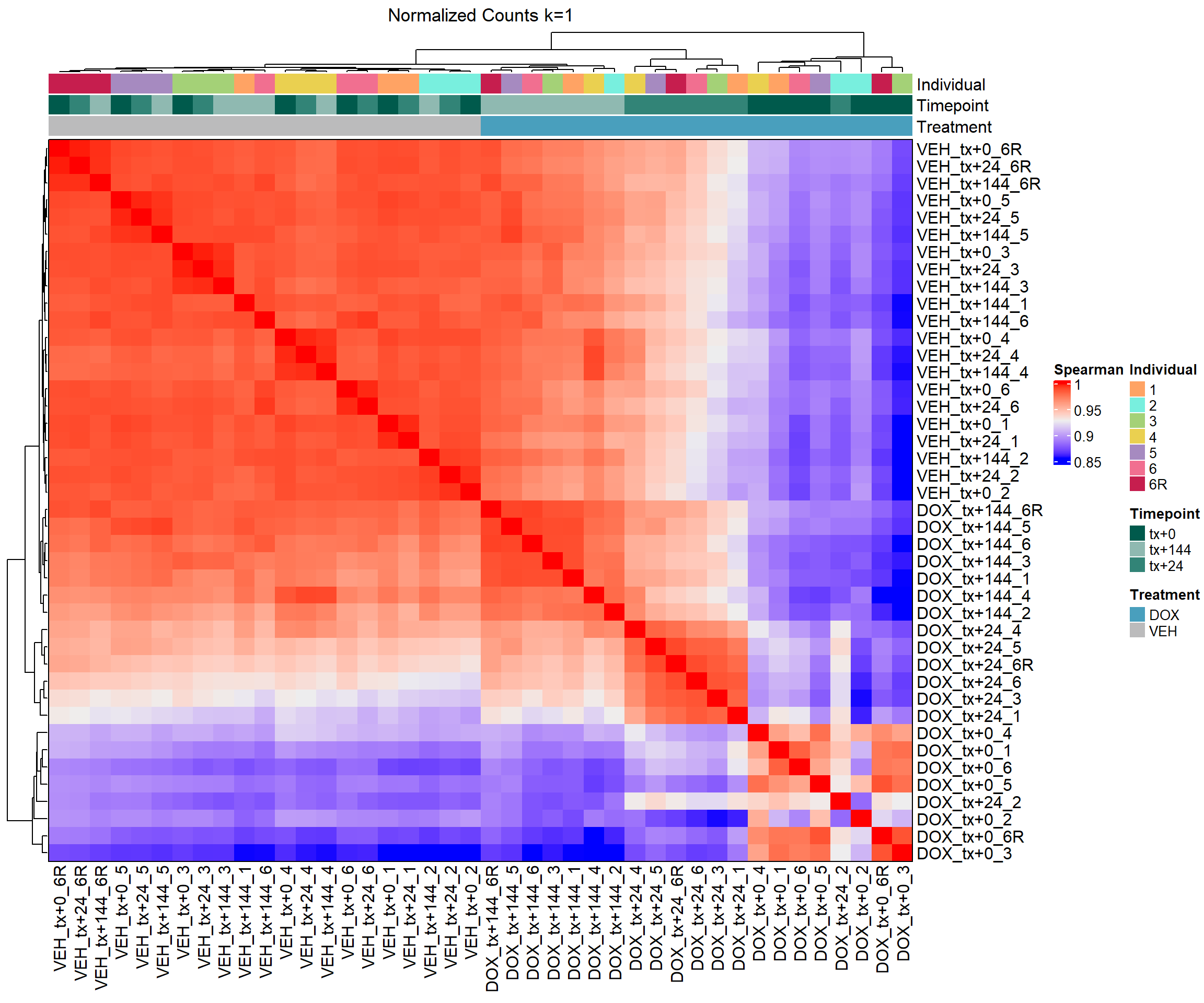
####Spearman Heatmap k=0 log2cpm####
heatmap_spmn_k0_cpm <- Heatmap(cor_matrix_spmn_k0_cpm,
                           name = "Spearman",
                           top_annotation = top_annotation,
                           show_row_names = TRUE,
                           show_column_names = TRUE,
                           cluster_rows = TRUE,
                           cluster_columns = TRUE,
                           border = TRUE,
                           column_title = "log2cpm of Filtered Counts no RUVs")

# Draw the heatmap k=0 log2cpm
draw(heatmap_spmn_k0_cpm)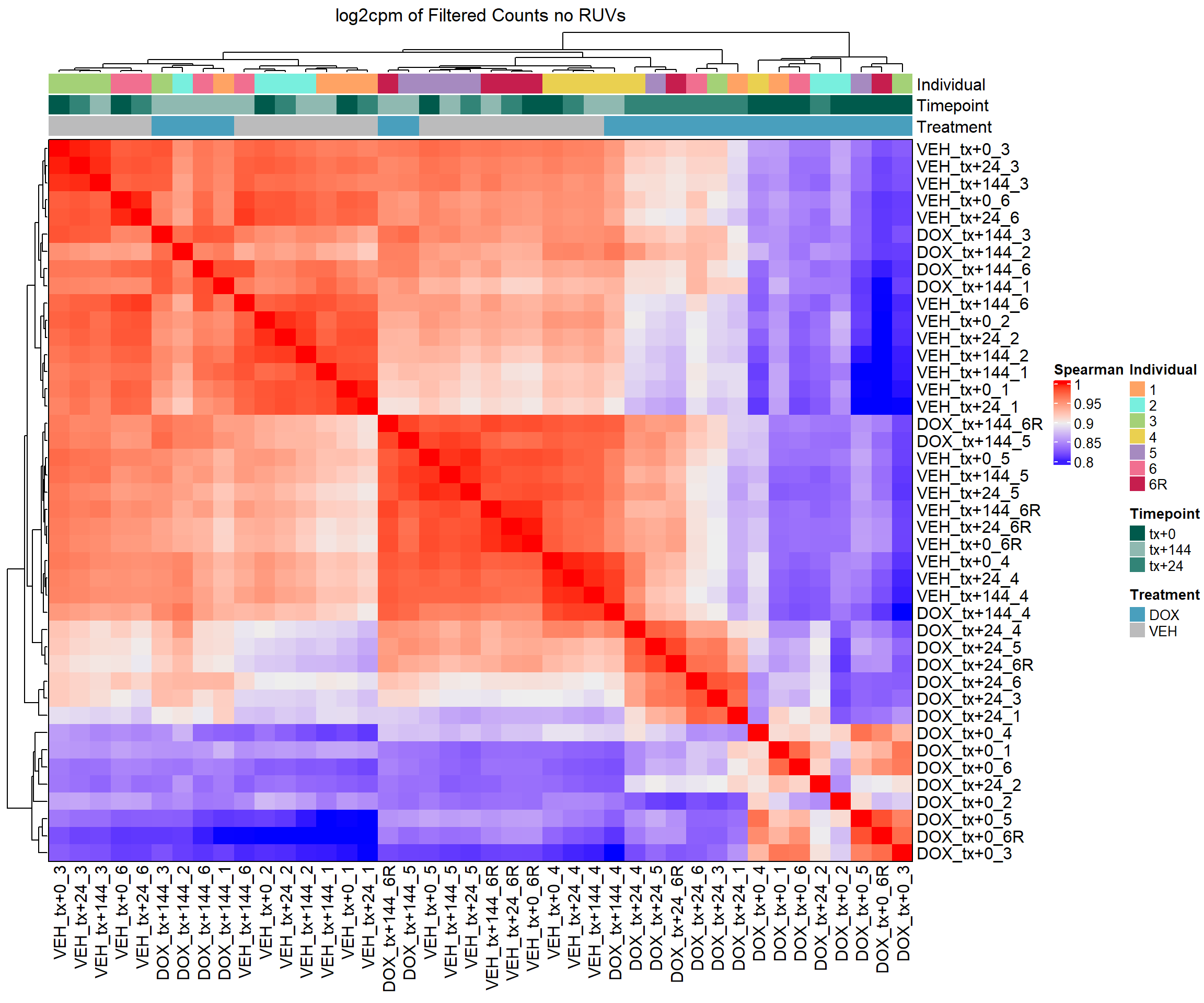
####Spearman Heatmap k=1 log2cpm####
heatmap_spmn_k1_cpm <- Heatmap(cor_matrix_spmn_k1_cpm,
                           name = "Spearman",
                           top_annotation = top_annotation,
                           show_row_names = TRUE,
                           show_column_names = TRUE,
                           cluster_rows = TRUE,
                           cluster_columns = TRUE,
                           border = TRUE,
                           column_title = "log2cpm of Normalized Counts k=1")

#draw the heatmap k=1 log2cpm
draw(heatmap_spmn_k1_cpm)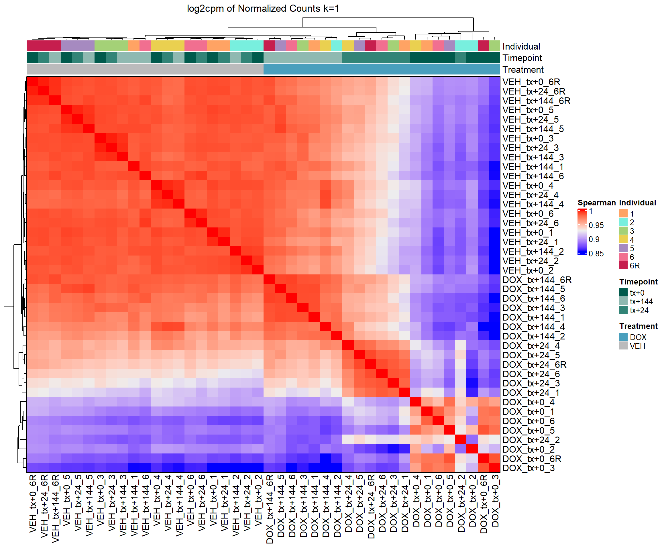
#find the median for all comparisons and also do a sign test to see significance
#remove diagonal (self-correlations) and get lower triangle only
spearman_vals <- cor_matrix_spmn_k1_cpm[lower.tri(cor_matrix_spmn_k1_cpm, diag = FALSE)]

#median of Spearman correlation coefficients
median_spearman <- median(spearman_vals, na.rm = TRUE)

#sign test: number of positive vs negative correlations
#H0: median = 0, HA: median > 0 (one-sided test)

#count number of positive and negative values
n_pos <- sum(spearman_vals > 0, na.rm = TRUE)
n_neg <- sum(spearman_vals < 0, na.rm = TRUE)
n_total <- n_pos + n_neg

#perform a binomial test (sign test)
sign_test <- binom.test(x = n_pos, n = n_total, p = 0.5, alternative = "greater")

#output results
cat("Median Spearman correlation:", median_spearman, "\n")
Median Spearman correlation: 0.9547968 cat("Sign test p-value (greater than 0):", sign_test$p.value, "\n")Sign test p-value (greater than 0): 6.503898e-260 #Median Spearman correlation: 0.9547968
#Sign test p-value (greater than 0): 6.503898e-260
#now I want to test correlations by timepoint with DOX vs DMSO
#list your timepoints
cor_time_sp <- c("tx+0", "tx+24", "tx+144")
for (tp in cor_time_sp) {
#match DOX and DMSO samples at this timepoint
dox_samples <- grep(paste0("^DOX_", tp), colnames(cor_matrix_spmn_k1_cpm), value = TRUE)
dmso_samples <- grep(paste0("^VEH_", tp), colnames(cor_matrix_spmn_k1_cpm), value = TRUE)
#extract Spearman correlations between DOX and DMSO at this timepoint
cor_vals <- as.vector(cor_matrix_spmn_k1_cpm[dox_samples, dmso_samples])
#calculate median
median_cor <- median(cor_vals, na.rm = TRUE)
#sign test (are most correlations > 0?)
n_pos <- sum(cor_vals > 0, na.rm = TRUE)
n_neg <- sum(cor_vals < 0, na.rm = TRUE)
n_total <- n_pos + n_neg
#perform binomial test if valid
if (n_total > 0) {
sign_test <- binom.test(x = n_pos, n = n_total, p = 0.5,
alternative = "greater")
p_val <- sign_test$p.value
} else {
p_val <- NA
}
#output
cat("====", tp, "====\n")
cat("Median Spearman correlation (DOX vs VEH):", round(median_cor, 4), "\n")
cat("Sign test p-value:", p_val, "\n\n")
}==== tx+0 ====
Median Spearman correlation (DOX vs VEH): NA
Sign test p-value: NA
==== tx+24 ====
Median Spearman correlation (DOX vs VEH): NA
Sign test p-value: NA
==== tx+144 ====
Median Spearman correlation (DOX vs VEH): NA
Sign test p-value: NA # output
# t0
# Median Spearman correlation (DOX vs VEH): 0.8899
# Sign test p-value: 1.776357e-15
#
# t24
# Median Spearman correlation (DOX vs VEH): 0.9347
# Sign test p-value: 1.776357e-15
#
# t144
# Median Spearman correlation (DOX vs VEH): 0.9767
# Sign test p-value: 1.776357e-15
#this means that my DOX and VEH are highly similar and significant according to P valuesSupplementary Figure 3 - Spearman Correlation Heatmap RUVs log2cpm
#Make your supplement heatmap
#rename your columns for your matrix cpm_k1 to be correct
# I RENAMED THESE EARLIER
# new_colname <- colnames(cpm_k1) %>%
# gsub("t0", "tx+0", .) %>%
# gsub("t24", "tx+24", .) %>%
# gsub("t144", "tx+144", .) %>%
# gsub("DMSO", "VEH", .)
# cpm_k1_rename <- cpm_k1
# colnames(cpm_k1_rename) <- new_colname
# cpm_k1 <- cpm_k1_rename
# saveRDS(cpm_k1, "data/QC/cpm_k1_renamedcols.RDS")
cor_matrix_spmn_k1_cpm_new <- cor(cpm_k1,
y = NULL,
use = "everything",
method = "spearman")
#create ComplexHeatmap
heatmap_spmn_supp <- Heatmap(
cor_matrix_spmn_k1_cpm,
name = "Spearman",
top_annotation = top_annotation,
show_row_names = TRUE,
show_column_names = TRUE,
cluster_rows = TRUE,
cluster_columns = TRUE,
show_row_dend = FALSE,
show_column_dend = TRUE,
row_names_gp = gpar(fontsize = 7),
column_names_gp = gpar(fontsize = 7),
column_names_centered = FALSE,
row_names_centered = FALSE,
rect_gp = gpar(col = "black", lwd = 0.5),
border = gpar(col = "black", lwd = 1),
column_title = "log2cpm of normalized counts RUVs corrected",
column_title_gp = gpar(fontsize = 10, fontface = "plain"),
heatmap_legend_param = list(
title_gp = gpar(fontsize = 9, fontface = "plain"),
labels_gp = gpar(fontsize = 8)
)
)
#make a function to save complex heatmaps
save_complex_heatmap <- function(plot, filename, folder, width = 6, height = 8) {
if (!dir.exists(folder)) dir.create(folder, recursive = TRUE)
path <- file.path(folder, filename)
pdf(path, width = width, height = height)
draw(plot, heatmap_legend_side = "right")
dev.off()
message("Saved heatmap to: ", path)
}
# Save to PDF in your output folder
save_complex_heatmap(
plot = heatmap_spmn_supp,
filename = "SuppFig3_SpearmanCorHM_RUV_log2cpm_EMP.pdf",
folder = output_folder,
width = 8,
height = 7
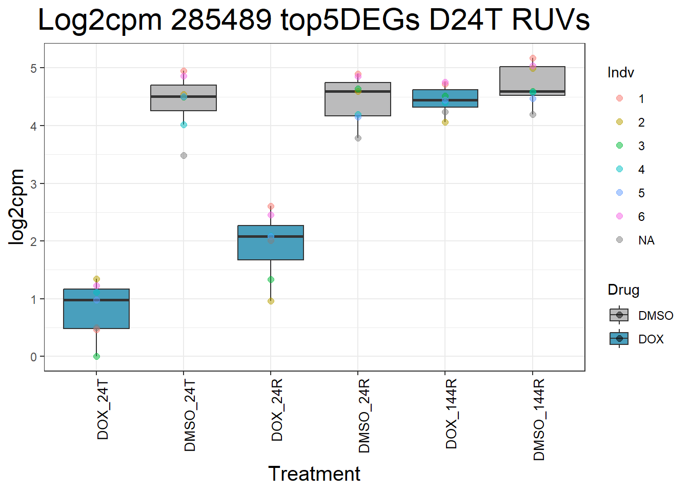
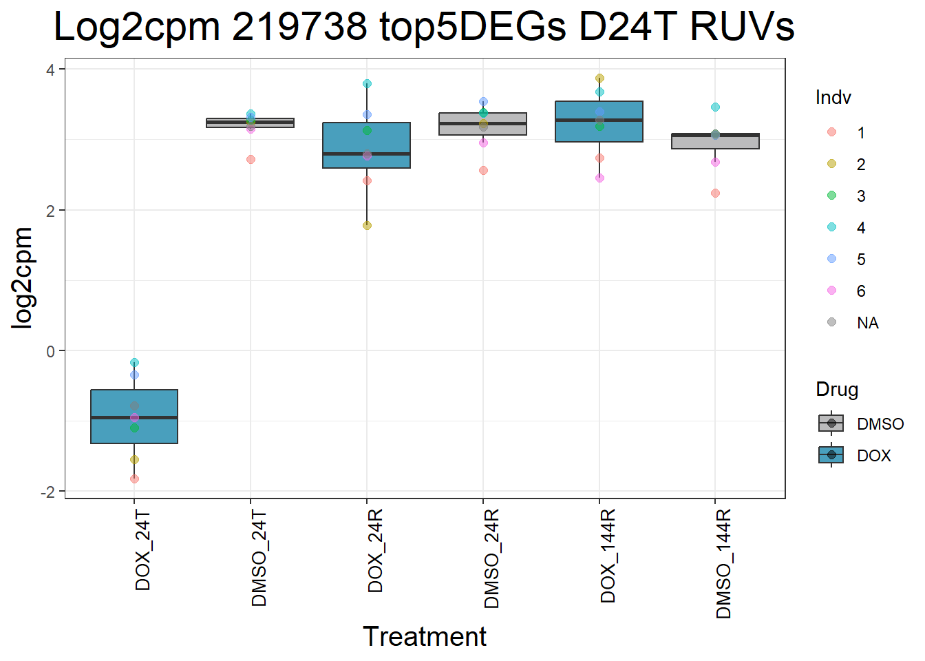
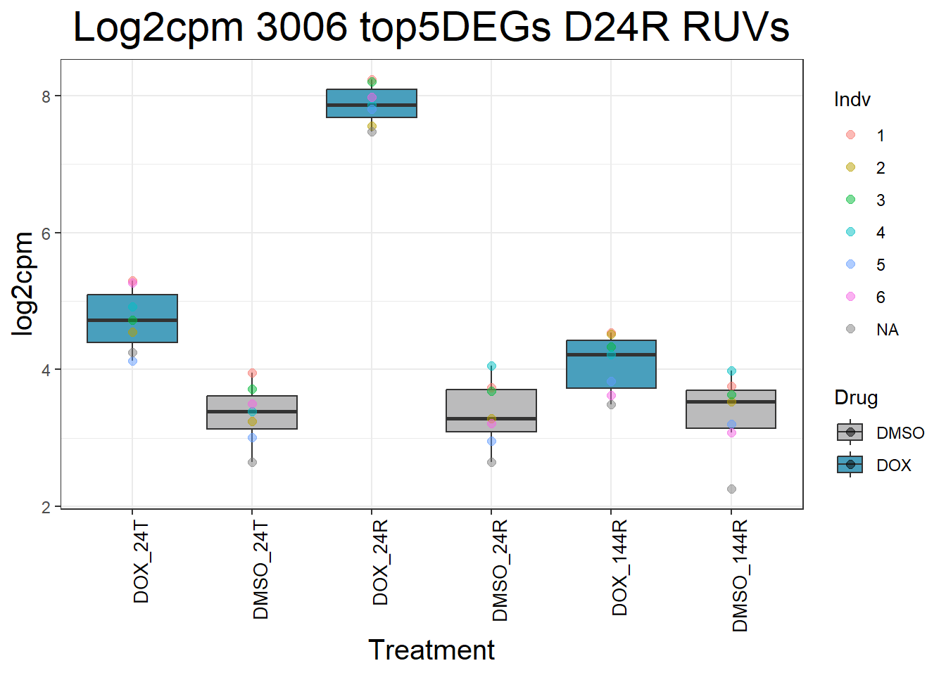
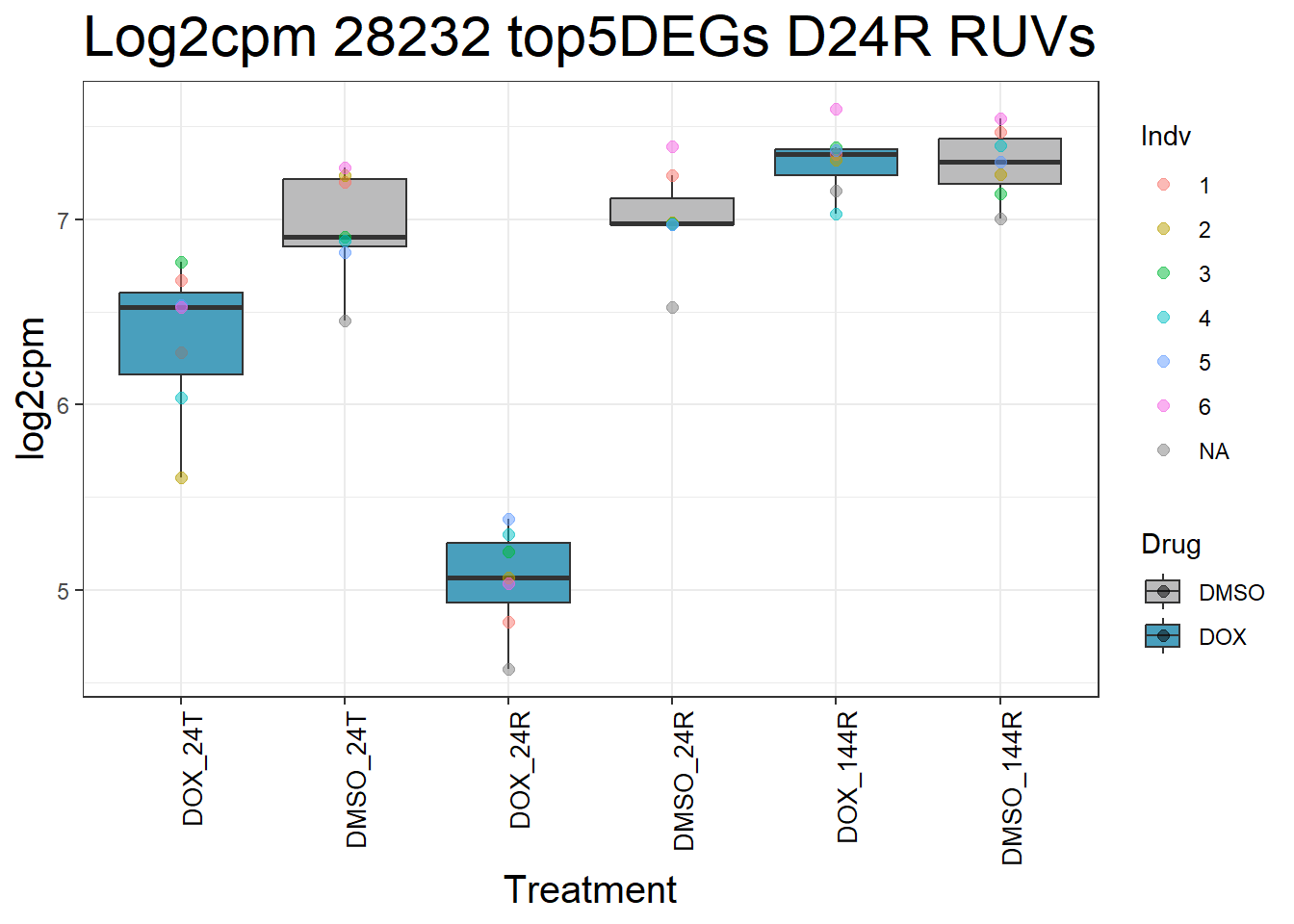
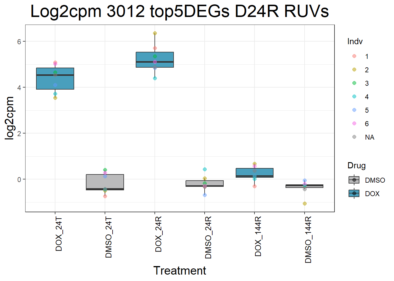
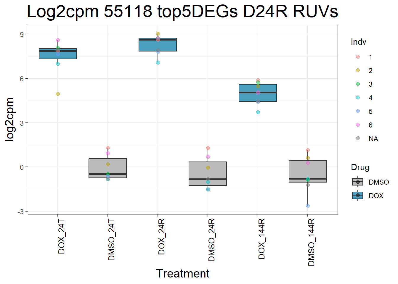
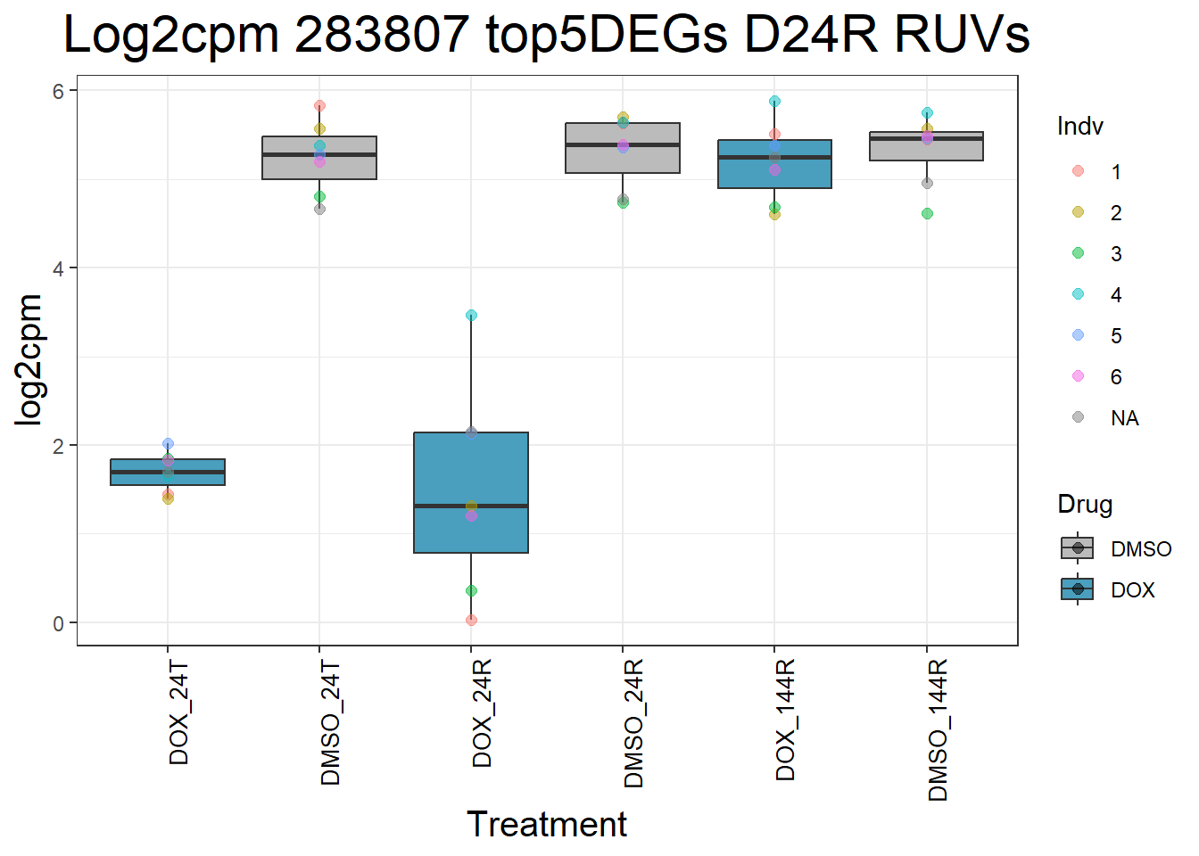
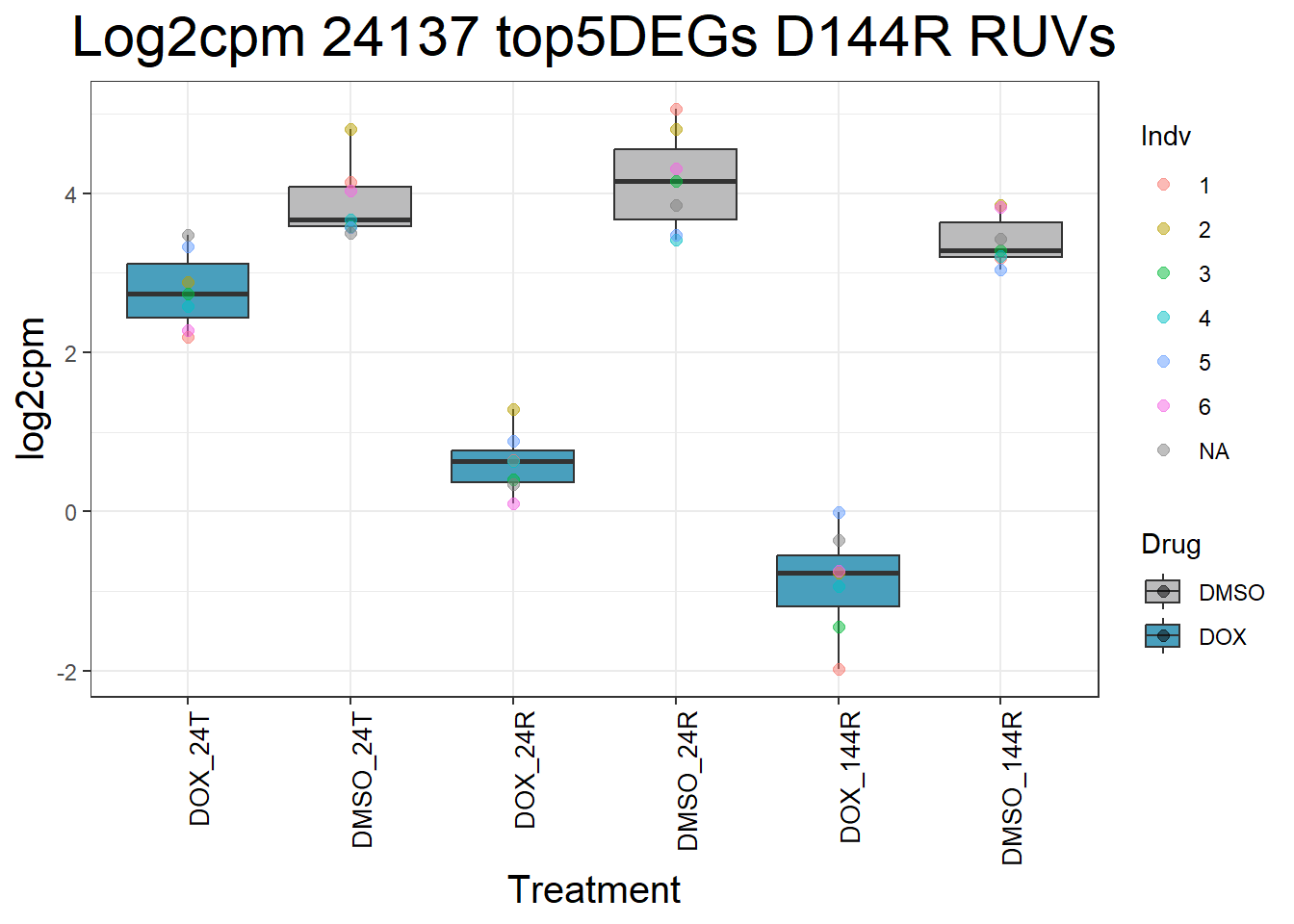
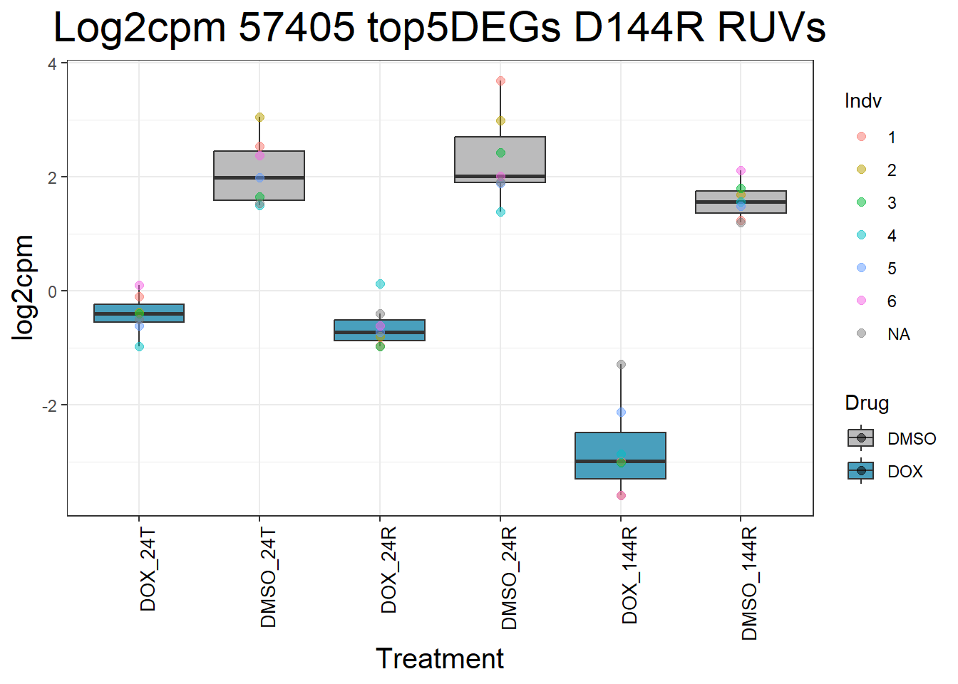
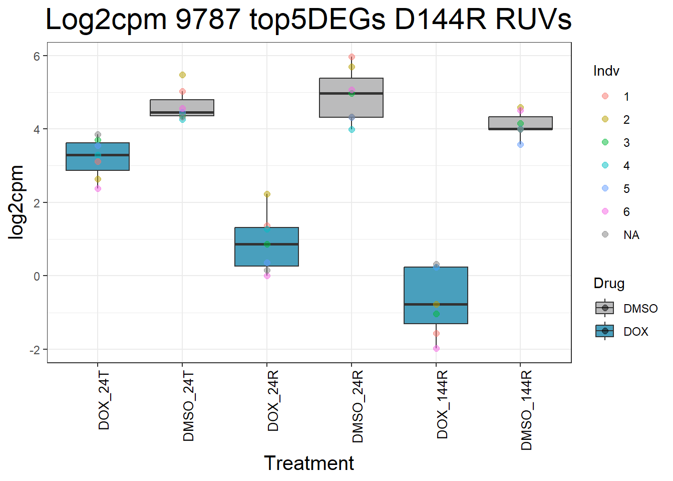
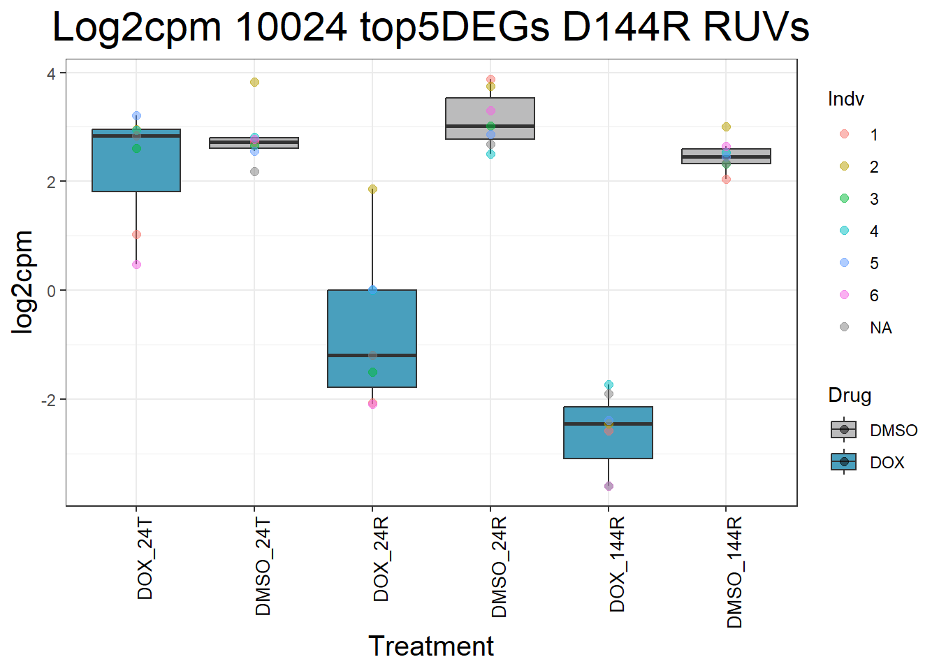
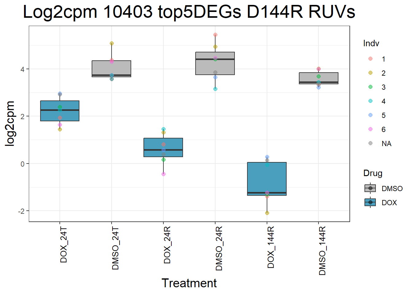
)Top 5 DEGs RUVs
#use your three toptables so I can pull out top 5 genes from each based on adj. p val

Toptable_RUV_24T <- read.csv("data/DE/Toptable_RUV_24T_final.csv")
Toptable_RUV_24R <- read.csv("data/DE/Toptable_RUV_24R_final.csv")
Toptable_RUV_144R <- read.csv("data/DE/Toptable_RUV_144R_final.csv")

top5_D24T_1 <- Toptable_RUV_24T[order(Toptable_RUV_24T$adj.P.Val), ][1:5,]
top5_D24R_1 <- Toptable_RUV_24R[order(Toptable_RUV_24R$adj.P.Val), ][1:5,]
top5_D144R_1 <- Toptable_RUV_144R[order(Toptable_RUV_144R$adj.P.Val), ][1:5,]

#now that I've pulled the top 5 DEGs from each, make a list to pull them from my log2cpm data

boxplot1 <- readRDS("data/QC/filcpm_matrix_genes.RDS") %>%
  as.data.frame()

#Define gene list
#these are the top 5 genes pulled from my toptables
top5_D24T_geneslist_1 <- c(top5_D24T_1$Entrez_ID)
top5_D24R_geneslist_1 <- c(top5_D24R_1$Entrez_ID)
top5_D144R_geneslist_1 <- c(top5_D144R_1$Entrez_ID)
#Add more gene symbols as needed or add more categories

#now pull these from my log2cpm matrix
top5_D24T_genes_1 <- boxplot1[boxplot1$Entrez_ID %in% top5_D24T_geneslist_1,]
dim(top5_D24T_genes_1)
[1] 5 44#5 genes in 44 cols
top5_D24R_genes_1 <- boxplot1[boxplot1$Entrez_ID %in% top5_D24R_geneslist_1,]
dim(top5_D24R_genes_1)[1] 5 44#5 genes in 44 cols
top5_D144R_genes_1 <- boxplot1[boxplot1$Entrez_ID %in% top5_D144R_geneslist_1,]
dim(top5_D144R_genes_1)[1] 5 44#5 genes in 44 cols
#Now put in the function I want to use to generate boxplots of genes
#####D24T#####
process_top5_D24T_1 <- function(gene) {
gene_data <- top5_D24T_genes_1 %>% filter(Entrez_ID == gene)
long_data <- gene_data %>%
pivot_longer(cols = -c(Entrez_ID, SYMBOL), names_to = "Sample", values_to = "log2cpm") %>%
mutate(
Drug = case_when(
grepl("DOX", Sample) ~ "DOX",
grepl("DMSO", Sample) ~ "DMSO",
TRUE ~ NA_character_
),
Timepoint = case_when(
grepl("_24T_", Sample) ~ "24T",
grepl("_24R_", Sample) ~ "24R",
grepl("_144R_", Sample) ~ "144R",
TRUE ~ NA_character_
),
Indv = case_when(
grepl("Ind1$", Sample) ~ "1",
grepl("Ind2$", Sample) ~ "2",
grepl("Ind3$", Sample) ~ "3",
grepl("Ind4$", Sample) ~ "4",
grepl("Ind5$", Sample) ~ "5",
grepl("Ind6$", Sample) ~ "6",
grepl("Ind6R$", Sample) ~ "6R",
TRUE ~ NA_character_
),
Condition = paste(Drug, Timepoint, sep = "_")
)
long_data$Condition <- factor(
long_data$Condition,
levels = c(
"DOX_24T",
"DMSO_24T",
"DOX_24R",
"DMSO_24R",
"DOX_144R",
"DMSO_144R"
)
)
return(long_data)
}
#Generate Boxplots from the above function using our gene list above
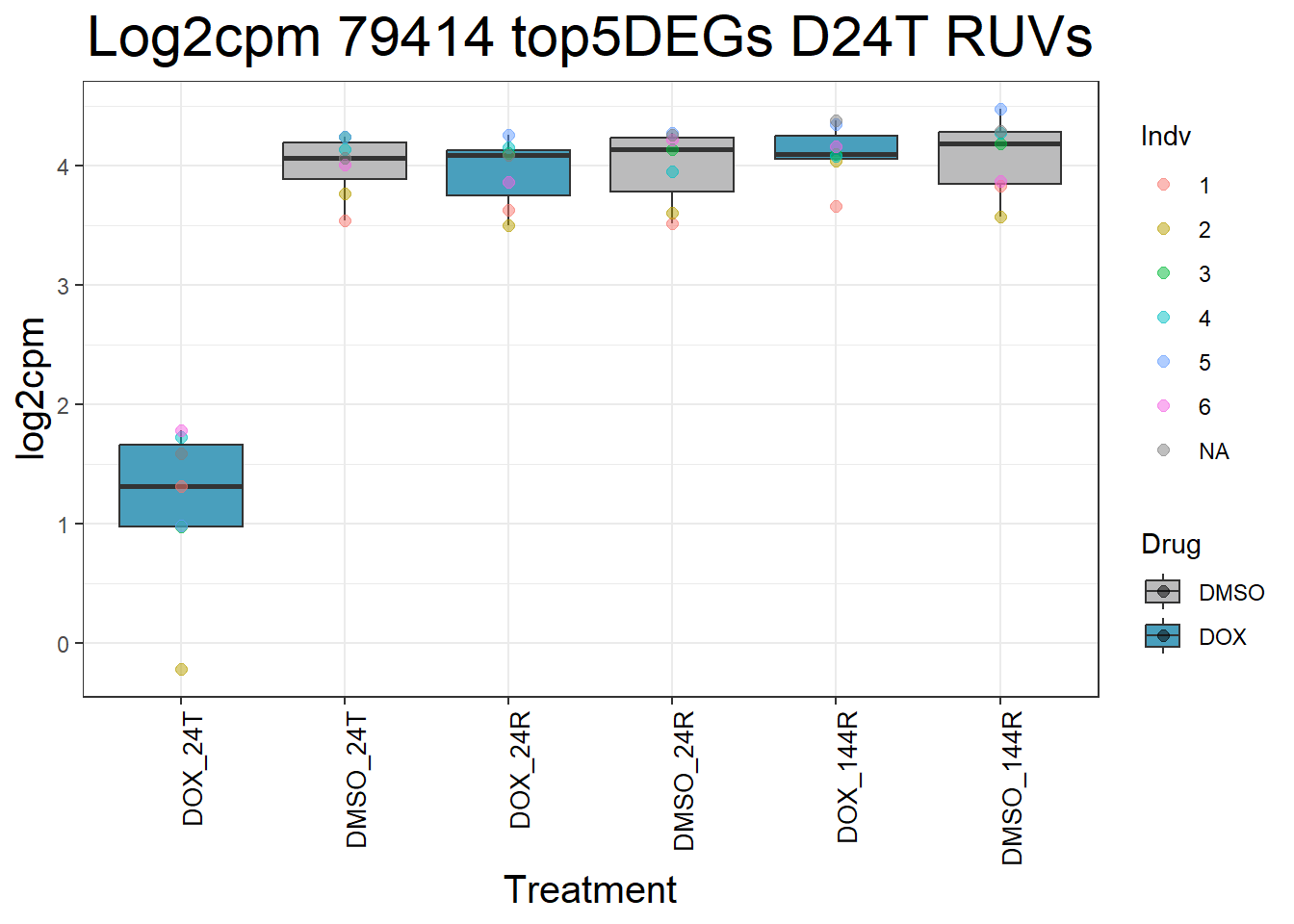
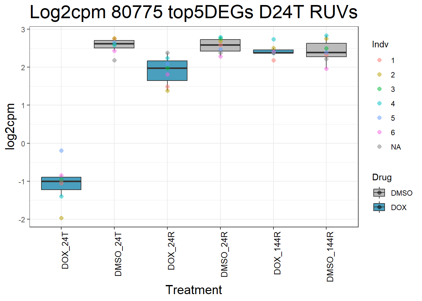
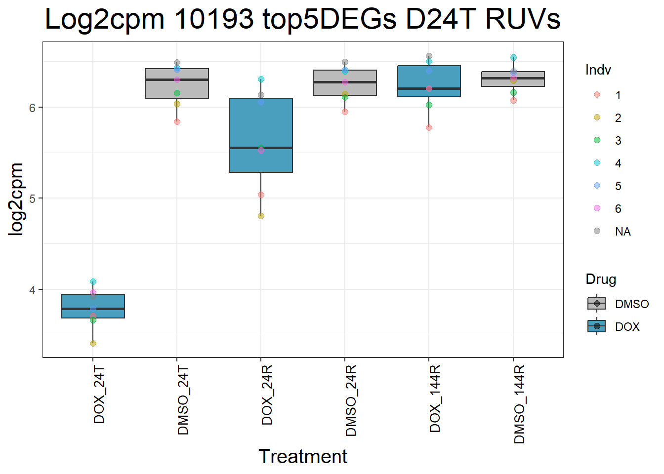
for (gene in top5_D24T_geneslist_1) {
gene_data <- process_top5_D24T_1(gene)
p <- ggplot(gene_data, aes(x = Condition, y = log2cpm, fill = Drug)) +
geom_boxplot(outlier.shape = NA) +
geom_point(aes(color = Indv), size = 2, alpha = 0.5, position = position_jitter(width = -1, height = 0)) +
scale_fill_manual(values = c("DOX" = "#499FBD", "DMSO" = "#BBBBBC")) +
ggtitle(paste("Log2cpm", gene, "top5DEGs D24T RUVs")) +
labs(x = "Treatment", y = "log2cpm") +
theme_bw() +
theme(
plot.title = element_text(size = rel(2), hjust = 0.5),
axis.title = element_text(size = 15, color = "black"),
axis.text.x = element_text(size = 10, color = "black", angle = 90, hjust = 1)
)
print(p)
}
#####D24R#####
process_top5_D24R_1 <- function(gene) {
  gene_data <- top5_D24R_genes_1 %>% filter(Entrez_ID == gene)
  long_data <- gene_data %>%
    pivot_longer(cols = -c(Entrez_ID, SYMBOL), names_to = "Sample", values_to = "log2cpm") %>%
    mutate(
      Drug = case_when(
        grepl("DOX", Sample) ~ "DOX",
        grepl("DMSO", Sample) ~ "DMSO",
        TRUE ~ NA_character_
      ),
      Timepoint = case_when(
        grepl("_24T_", Sample) ~ "24T",
        grepl("_24R_", Sample) ~ "24R",
        grepl("_144R_", Sample) ~ "144R",
        TRUE ~ NA_character_
      ),
      Indv = case_when(
        grepl("Ind1$", Sample) ~ "1",
        grepl("Ind2$", Sample) ~ "2",
        grepl("Ind3$", Sample) ~ "3",
        grepl("Ind4$", Sample) ~ "4",
        grepl("Ind5$", Sample) ~ "5",
        grepl("Ind6$", Sample) ~ "6",
        grepl("Ind6R$", Sample) ~ "6R",
        TRUE ~ NA_character_
      ),
      Condition = paste(Drug, Timepoint, sep = "_")
    )
  long_data$Condition <- factor(
    long_data$Condition,
    levels = c(
      "DOX_24T",
      "DMSO_24T",
      "DOX_24R",
      "DMSO_24R",
      "DOX_144R",
      "DMSO_144R"
    )
  )
  return(long_data)
}


#Generate Boxplots from the above function using our gene list above
for (gene in top5_D24R_geneslist_1) {
  gene_data <- process_top5_D24R_1(gene)
  p <- ggplot(gene_data, aes(x = Condition, y = log2cpm, fill = Drug)) +
    geom_boxplot(outlier.shape = NA) +
    geom_point(aes(color = Indv), size = 2, alpha = 0.5, position = position_jitter(width = -1, height = 0)) +
    scale_fill_manual(values = c("DOX" = "#499FBD", "DMSO" = "#BBBBBC")) +
    ggtitle(paste("Log2cpm", gene, "top5DEGs D24R RUVs")) +
    labs(x = "Treatment", y = "log2cpm") +
    theme_bw() +
    theme(
      plot.title = element_text(size = rel(2), hjust = 0.5),
      axis.title = element_text(size = 15, color = "black"),
      axis.text.x = element_text(size = 10, color = "black", angle = 90, hjust = 1)
    )
  print(p)
}
#####D144R#####
process_top5_D144R_1 <- function(gene) {
  gene_data <- top5_D144R_genes_1 %>% filter(Entrez_ID == gene)
  long_data <- gene_data %>%
    pivot_longer(cols = -c(Entrez_ID, SYMBOL), names_to = "Sample", values_to = "log2cpm") %>%
    mutate(
      Drug = case_when(
        grepl("DOX", Sample) ~ "DOX",
        grepl("DMSO", Sample) ~ "DMSO",
        TRUE ~ NA_character_
      ),
      Timepoint = case_when(
        grepl("_24T_", Sample) ~ "24T",
        grepl("_24R_", Sample) ~ "24R",
        grepl("_144R_", Sample) ~ "144R",
        TRUE ~ NA_character_
      ),
      Indv = case_when(
        grepl("Ind1$", Sample) ~ "1",
        grepl("Ind2$", Sample) ~ "2",
        grepl("Ind3$", Sample) ~ "3",
        grepl("Ind4$", Sample) ~ "4",
        grepl("Ind5$", Sample) ~ "5",
        grepl("Ind6$", Sample) ~ "6",
        grepl("Ind6R$", Sample) ~ "6R",
        TRUE ~ NA_character_
      ),
      Condition = paste(Drug, Timepoint, sep = "_")
    )
  long_data$Condition <- factor(
    long_data$Condition,
    levels = c(
      "DOX_24T",
      "DMSO_24T",
      "DOX_24R",
      "DMSO_24R",
      "DOX_144R",
      "DMSO_144R"
    )
  )
  return(long_data)
}


#Generate Boxplots from the above function using our gene list above
for (gene in top5_D144R_geneslist_1) {
  gene_data <- process_top5_D144R_1(gene)
  p <- ggplot(gene_data, aes(x = Condition, y = log2cpm, fill = Drug)) +
    geom_boxplot(outlier.shape = NA) +
    geom_point(aes(color = Indv), size = 2, alpha = 0.5, position = position_jitter(width = -1, height = 0)) +
    scale_fill_manual(values = c("DOX" = "#499FBD", "DMSO" = "#BBBBBC")) +
    ggtitle(paste("Log2cpm", gene, "top5DEGs D144R RUVs")) +
    labs(x = "Treatment", y = "log2cpm") +
    theme_bw() +
    theme(
      plot.title = element_text(size = rel(2), hjust = 0.5),
      axis.title = element_text(size = 15, color = "black"),
      axis.text.x = element_text(size = 10, color = "black", angle = 90, hjust = 1)
    )
  print(p)
}
sessionInfo()R version 4.4.2 (2024-10-31 ucrt)
Platform: x86_64-w64-mingw32/x64
Running under: Windows 11 x64 (build 22000)
Matrix products: default
locale:
[1] LC_COLLATE=English_United States.utf8
[2] LC_CTYPE=English_United States.utf8
[3] LC_MONETARY=English_United States.utf8
[4] LC_NUMERIC=C
[5] LC_TIME=English_United States.utf8
time zone: America/Chicago
tzcode source: internal
attached base packages:
[1] grid stats4 stats graphics grDevices utils datasets
[8] methods base
other attached packages:
[1] ggrepel_0.9.6 ComplexHeatmap_2.22.0
[3] ggfortify_0.4.17 readxl_1.4.5
[5] lubridate_1.9.4 forcats_1.0.0
[7] stringr_1.5.1 dplyr_1.1.4
[9] purrr_1.0.4 readr_2.1.5
[11] tidyr_1.3.1 tibble_3.2.1
[13] ggplot2_3.5.2 tidyverse_2.0.0
[15] RUVSeq_1.40.0 edgeR_4.4.0
[17] limma_3.62.1 EDASeq_2.40.0
[19] ShortRead_1.64.0 GenomicAlignments_1.42.0
[21] SummarizedExperiment_1.36.0 MatrixGenerics_1.18.1
[23] matrixStats_1.5.0 Rsamtools_2.22.0
[25] GenomicRanges_1.58.0 Biostrings_2.74.0
[27] GenomeInfoDb_1.42.3 XVector_0.46.0
[29] IRanges_2.40.0 S4Vectors_0.44.0
[31] BiocParallel_1.40.0 Biobase_2.66.0
[33] BiocGenerics_0.52.0 workflowr_1.7.1
loaded via a namespace (and not attached):
[1] RColorBrewer_1.1-3 shape_1.4.6.1 rstudioapi_0.17.1
[4] jsonlite_2.0.0 magrittr_2.0.3 magick_2.9.0
[7] GenomicFeatures_1.58.0 farver_2.1.2 rmarkdown_2.29
[10] GlobalOptions_0.1.2 fs_1.6.6 BiocIO_1.16.0
[13] zlibbioc_1.52.0 vctrs_0.6.5 Cairo_1.6-5
[16] memoise_2.0.1 RCurl_1.98-1.17 htmltools_0.5.8.1
[19] S4Arrays_1.6.0 progress_1.2.3 curl_6.0.1
[22] cellranger_1.1.0 SparseArray_1.6.0 sass_0.4.10
[25] bslib_0.9.0 httr2_1.1.2 cachem_1.1.0
[28] whisker_0.4.1 iterators_1.0.14 lifecycle_1.0.4
[31] pkgconfig_2.0.3 Matrix_1.7-1 R6_2.6.1
[34] fastmap_1.2.0 clue_0.3-66 GenomeInfoDbData_1.2.13
[37] digest_0.6.37 colorspace_2.1-1 AnnotationDbi_1.68.0
[40] ps_1.9.1 rprojroot_2.0.4 RSQLite_2.3.9
[43] hwriter_1.3.2.1 labeling_0.4.3 filelock_1.0.3
[46] timechange_0.3.0 httr_1.4.7 abind_1.4-8
[49] compiler_4.4.2 doParallel_1.0.17 bit64_4.5.2
[52] withr_3.0.2 DBI_1.2.3 R.utils_2.13.0
[55] biomaRt_2.62.1 MASS_7.3-61 rappdirs_0.3.3
[58] DelayedArray_0.32.0 rjson_0.2.23 tools_4.4.2
[61] httpuv_1.6.16 R.oo_1.27.1 glue_1.8.0
[64] restfulr_0.0.15 callr_3.7.6 promises_1.3.2
[67] getPass_0.2-4 cluster_2.1.6 generics_0.1.4
[70] gtable_0.3.6 tzdb_0.5.0 R.methodsS3_1.8.2
[73] hms_1.1.3 xml2_1.3.8 foreach_1.5.2
[76] pillar_1.10.2 later_1.4.2 circlize_0.4.16
[79] BiocFileCache_2.14.0 lattice_0.22-6 aroma.light_3.36.0
[82] rtracklayer_1.66.0 bit_4.5.0 deldir_2.0-4
[85] tidyselect_1.2.1 locfit_1.5-9.12 knitr_1.50
[88] git2r_0.36.2 gridExtra_2.3 xfun_0.52
[91] statmod_1.5.0 stringi_1.8.7 UCSC.utils_1.2.0
[94] yaml_2.3.10 evaluate_1.0.3 codetools_0.2-20
[97] interp_1.1-6 cli_3.6.3 processx_3.8.6
[100] jquerylib_0.1.4 Rcpp_1.0.14 dbplyr_2.5.0
[103] png_0.1-8 XML_3.99-0.18 parallel_4.4.2
[106] blob_1.2.4 prettyunits_1.2.0 latticeExtra_0.6-30
[109] jpeg_0.1-11 bitops_1.0-9 pwalign_1.2.0
[112] scales_1.4.0 crayon_1.5.3 GetoptLong_1.0.5
[115] rlang_1.1.6 KEGGREST_1.46.0