Figure 2 Analysis
Last updated: 2026-01-06
Checks: 7 0
Knit directory: DXR_website/
This reproducible R Markdown analysis was created with workflowr (version 1.7.1). The Checks tab describes the reproducibility checks that were applied when the results were created. The Past versions tab lists the development history.
Great! Since the R Markdown file has been committed to the Git repository, you know the exact version of the code that produced these results.
Great job! The global environment was empty. Objects defined in the global environment can affect the analysis in your R Markdown file in unknown ways. For reproduciblity it’s best to always run the code in an empty environment.
The command set.seed(20251201) was run prior to running
the code in the R Markdown file. Setting a seed ensures that any results
that rely on randomness, e.g. subsampling or permutations, are
reproducible.
Great job! Recording the operating system, R version, and package versions is critical for reproducibility.
Nice! There were no cached chunks for this analysis, so you can be confident that you successfully produced the results during this run.
Great job! Using relative paths to the files within your workflowr project makes it easier to run your code on other machines.
Great! You are using Git for version control. Tracking code development and connecting the code version to the results is critical for reproducibility.
The results in this page were generated with repository version e4705f6. See the Past versions tab to see a history of the changes made to the R Markdown and HTML files.
Note that you need to be careful to ensure that all relevant files for
the analysis have been committed to Git prior to generating the results
(you can use wflow_publish or
wflow_git_commit). workflowr only checks the R Markdown
file, but you know if there are other scripts or data files that it
depends on. Below is the status of the Git repository when the results
were generated:
Ignored files:
    Ignored:    .Rhistory
    Ignored:    .Rproj.user/
    Ignored:    DXR_website/data/
    Ignored:    code/Flow_Purity_Stressor_Boxplots_EMP_250226.R
    Ignored:    data/CDKN1A_geneplot_Dox.RDS
    Ignored:    data/Cormotif_dox.RDS
    Ignored:    data/Cormotif_prob_gene_list.RDS
    Ignored:    data/Cormotif_prob_gene_list_doxonly.RDS
    Ignored:    data/Counts_RNA_EMPfortmiller.txt
    Ignored:    data/DMSO_TNN13_plot.RDS
    Ignored:    data/DOX_TNN13_plot.RDS
    Ignored:    data/DOXgeneplots.RDS
    Ignored:    data/ExpressionMatrix_EMP.csv
    Ignored:    data/Ind1_DOX_Spearman_plot.RDS
    Ignored:    data/Ind6REP_Spearman_list.csv
    Ignored:    data/Ind6REP_Spearman_plot.RDS
    Ignored:    data/Ind6REP_Spearman_set.csv
    Ignored:    data/Ind6_Spearman_plot.RDS
    Ignored:    data/MDM2_geneplot_Dox.RDS
    Ignored:    data/Master_summary_75-1_EMP_250811_final.csv
    Ignored:    data/Master_summary_87-1_EMP_250811_final.csv
    Ignored:    data/Metadata.csv
    Ignored:    data/Metadata_2_norep_update.RDS
    Ignored:    data/Metadata_update.csv
    Ignored:    data/QC/
    Ignored:    data/Recovery_flow_purity.csv
    Ignored:    data/SIRT1_geneplot_Dox.RDS
    Ignored:    data/Sample_annotated.csv
    Ignored:    data/SpearmanHeatmapMatrix_EMP
    Ignored:    data/VolcanoPlot_D144R_original_EMP_250623.png
    Ignored:    data/VolcanoPlot_D24R_original_EMP_250623.png
    Ignored:    data/VolcanoPlot_D24T_original_EMP_250623.png
    Ignored:    data/annot_dox.RDS
    Ignored:    data/annot_list_hm.csv
    Ignored:    data/cormotif_dxr_1.RDS
    Ignored:    data/cormotif_dxr_2.RDS
    Ignored:    data/counts/
    Ignored:    data/counts_DE_df_dox.RDS
    Ignored:    data/counts_DE_raw_data.RDS
    Ignored:    data/counts_raw_filt.RDS
    Ignored:    data/counts_raw_matrix.RDS
    Ignored:    data/counts_raw_matrix_EMP_250514.csv
    Ignored:    data/d24_Spearman_plot.RDS
    Ignored:    data/dge_calc_dxr.RDS
    Ignored:    data/dge_calc_matrix.RDS
    Ignored:    data/ensembl_backup_dox.RDS
    Ignored:    data/fC_AllCounts.RDS
    Ignored:    data/fC_DOXCounts.RDS
    Ignored:    data/featureCounts_Concat_Matrix_DOXSamples_EMP_250430.csv
    Ignored:    data/featureCounts_DOXdata_updatedind.RDS
    Ignored:    data/filcpm_colnames_matrix.csv
    Ignored:    data/filcpm_matrix.csv
    Ignored:    data/filt_gene_list_dox.RDS
    Ignored:    data/filter_gene_list_final.RDS
    Ignored:    data/final_data/
    Ignored:    data/gene_clustlike_motif.RDS
    Ignored:    data/gene_postprob_motif.RDS
    Ignored:    data/genedf_dxr.RDS
    Ignored:    data/genematrix_dox.RDS
    Ignored:    data/genematrix_dxr.RDS
    Ignored:    data/heartgenes.csv
    Ignored:    data/heartgenes_dox.csv
    Ignored:    data/image_intensity_stats_all_conditions.csv
    Ignored:    data/image_level_stats_all_conditions.csv
    Ignored:    data/image_level_summary_yH2AX_quant.csv
    Ignored:    data/ind_num_dox.RDS
    Ignored:    data/ind_num_dxr.RDS
    Ignored:    data/initial_cormotif.RDS
    Ignored:    data/initial_cormotif_dox.RDS
    Ignored:    data/low_nuclei_samples.csv
    Ignored:    data/low_veh_samples.csv
    Ignored:    data/new/
    Ignored:    data/new_cormotif_dox.RDS
    Ignored:    data/perc_mean_all_10X.png
    Ignored:    data/perc_mean_all_20X.png
    Ignored:    data/perc_mean_all_40X.png
    Ignored:    data/perc_mean_consistent_10X.png
    Ignored:    data/perc_mean_consistent_20X.png
    Ignored:    data/perc_mean_consistent_40X.png
    Ignored:    data/perc_median_all_10X.png
    Ignored:    data/perc_median_all_20X.png
    Ignored:    data/perc_median_all_40X.png
    Ignored:    data/perc_median_consistent_10X.png
    Ignored:    data/perc_median_consistent_20X.png
    Ignored:    data/perc_median_consistent_40X.png
    Ignored:    data/plot_leg_d.RDS
    Ignored:    data/plot_leg_d_horizontal.RDS
    Ignored:    data/plot_leg_d_vertical.RDS
    Ignored:    data/plot_theme_custom.RDS
    Ignored:    data/process_gene_data_funct.RDS
    Ignored:    data/raw_mean_all_10X.png
    Ignored:    data/raw_mean_all_20X.png
    Ignored:    data/raw_mean_all_40X.png
    Ignored:    data/raw_mean_consistent_10X.png
    Ignored:    data/raw_mean_consistent_20X.png
    Ignored:    data/raw_mean_consistent_40X.png
    Ignored:    data/raw_median_all_10X.png
    Ignored:    data/raw_median_all_20X.png
    Ignored:    data/raw_median_all_40X.png
    Ignored:    data/raw_median_consistent_10X.png
    Ignored:    data/raw_median_consistent_20X.png
    Ignored:    data/raw_median_consistent_40X.png
    Ignored:    data/ruv/
    Ignored:    data/summary_all_IF_ROI.RDS
    Ignored:    data/tableED_GOBP.RDS
    Ignored:    data/tableESR_GOBP_postprob.RDS
    Ignored:    data/tableLD_GOBP.RDS
    Ignored:    data/tableLR_GOBP_postprob.RDS
    Ignored:    data/tableNR_GOBP.RDS
    Ignored:    data/tableNR_GOBP_postprob.RDS
    Ignored:    data/table_incsus_genes_GOBP_RUV.RDS
    Ignored:    data/table_motif1_GOBP_d.RDS
    Ignored:    data/table_motif1_genes_GOBP.RDS
    Ignored:    data/table_motif2_GOBP_d.RDS
    Ignored:    data/table_motif3_genes_GOBP.RDS
    Ignored:    data/thing.R
    Ignored:    data/top.table_V.D144r_dox.RDS
    Ignored:    data/top.table_V.D24_dox.RDS
    Ignored:    data/top.table_V.D24r_dox.RDS
    Ignored:    data/yH2AX_75-1_EMP_250811.csv
    Ignored:    data/yH2AX_87-1_EMP_250811.csv
    Ignored:    data/yH2AX_Boxplots_MeanIntensity_10X_EMP_250811.png
    Ignored:    data/yH2AX_Boxplots_MeanIntensity_10X_NormtoMax_EMP_250811.png
    Ignored:    data/yH2AX_Boxplots_MeanIntensity_20X_EMP_250811.png
    Ignored:    data/yH2AX_Boxplots_MeanIntensity_20X_NormtoMax_EMP_250811.png
    Ignored:    data/yH2AX_Boxplots_MedianIntensity_10X_NormtoMax_EMP_250811.png
    Ignored:    data/yH2AX_Boxplots_MedianIntensity_20X_NormtoMax_EMP_250811.png
    Ignored:    data/yH2AX_Boxplots_MedianIntensity_NormtoMax_EMP_250811.png
    Ignored:    data/yH2AX_Boxplots_Quant_10X_EMP_250817.png
    Ignored:    data/yH2AX_Boxplots_Quant_20X_EMP_250817.png
    Ignored:    data/yh2ax_all_df_EMP_250812.csv
Note that any generated files, e.g. HTML, png, CSS, etc., are not included in this status report because it is ok for generated content to have uncommitted changes.
These are the previous versions of the repository in which changes were
made to the R Markdown (DXR_website/analysis/Figure2.Rmd)
and HTML (DXR_website/docs/Figure2.html) files. If you’ve
configured a remote Git repository (see ?wflow_git_remote),
click on the hyperlinks in the table below to view the files as they
were in that past version.
| File | Version | Author | Date | Message |
|---|---|---|---|---|
| html | c382b38 | emmapfort | 2026-01-06 | Build site. |
| Rmd | cd535e9 | emmapfort | 2026-01-06 | Final Website Touches 01/06/25 EMP |
| html | 7f22593 | emmapfort | 2026-01-05 | Build site. |
| Rmd | 49fa865 | emmapfort | 2026-01-05 | Final Updates to Website EMP 01/05/26 |
| html | f088a00 | emmapfort | 2025-12-09 | website updates |
| Rmd | e05f0cc | emmapfort | 2025-12-09 | workflowr::wflow_publish(files = c("analysis/Figure2.Rmd", "analysis/about.Rmd", |
| Rmd | a967d53 | emmapfort | 2025-12-09 | Update website and analysis chunks |
| html | a967d53 | emmapfort | 2025-12-09 | Update website and analysis chunks |
| Rmd | da1f69c | emmapfort | 2025-12-02 | updated analysis 12/02/25 |
Libraries
Load necessary libraries for analysis.
library(tidyverse)
library(readxl)
library(readr)
library(ggrepel)
library(ggfortify)
library(RUVSeq)
library(patchwork)
library(eulerr)
library(org.Hs.eg.db)
library(AnnotationDbi)
library(ggVennDiagram)
library(ggrastr)
Define my custom plot theme
# Define the custom theme
# plot_theme_custom <- function() {
#   theme_minimal() +
#     theme(
#       #line for x and y axis
#       axis.line = element_line(linewidth = 1,
#                                color = "black"),
#
#       #axis ticks only on x and y, length standard
#       axis.ticks.x = element_line(color = "black",
#                                 linewidth = 1),
#       axis.ticks.y = element_line(color = "black",
#                                 linewidth = 1),
#       axis.ticks.length = unit(0.05, "in"),
#
#       #text and font
#       axis.text = element_text(color = "black",
#                                family = "Arial",
#                                size = 7),
#       axis.title = element_text(color = "black",
#                                 family = "Arial",
#                                 size = 9),
#       legend.text = element_text(color = "black",
#                                  family = "Arial",
#                                  size = 7),
#       legend.title = element_text(color = "black",
#                                   family = "Arial",
#                                   size = 9),
#       plot.title = element_text(color = "black",
#                                 family = "Arial",
#                                 size = 10),
#
#       #blank background and border
#       panel.background = element_blank(),
#       panel.border = element_blank(),
#
#       #gridlines for alignment
#       panel.grid.major = element_line(color = "grey80", linewidth = 0.5),  #grey major grid for align in illus
#       panel.grid.minor = element_line(color = "grey90", linewidth = 0.5) #grey minor grid for align in illus
#     )
# }

# saveRDS(plot_theme_custom, "data/plot_theme_custom.RDS")

theme_custom <- readRDS("data/plot_theme_custom.RDS")
####Colors####
# txtime_col_old <- list(
# "DOX_24T" = "#263CA5",
# "VEH_24T" = "#444343",
# "DOX_24R" = "#5B8FD1",
# "VEH_24R" = "#757575",
# "DOX_144R" = "#89C5E5",
# "VEH_144R" = "#AAAAAA"
# )
#updated colors and factors:
ind_col <- list(
"1" = "#FF9F64",
"2" = "#78EBDA",
"3" = "#ADCD77",
"4" = "#E6CC50",
"5" = "#A68AC0",
"6" = "#F16F90",
"6R" = "#C61E4E"
)
ind_col_nr <- list(
"1" = "#FF9F64",
"2" = "#78EBDA",
"3" = "#ADCD77",
"4" = "#E6CC50",
"5" = "#A68AC0",
"6" = "#F16F90"
)
time_col <- list(
"t0" = "#005A4C",
"t24" = "#328477",
"t144" = "#8FB9B1")
tx_col <- list(
"DOX" = "#499FBD",
"VEH" = "#BBBBBC")
txtime_col <- list(
"DOX_t0" = "#263CA5",
"VEH_t0" = "#444343",
"DOX_t24" = "#5B8FD1",
"VEH_t24" = "#757575",
"DOX_t144" = "#89C5E5",
"VEH_t144" = "#AAAAAA"
)Define a function to save plots as .pdf and .png
save_plot <- function(plot, filename,
                      folder = ".",
                      width = 8,
                      height = 6,
                      units = "in",
                      dpi = 300,
                      add_date = TRUE) {
  if (missing(filename)) stop("Please provide a filename (without extension) for the plot.")

  date_str <- if (add_date) paste0("_", format(Sys.Date(), "%y%m%d")) else ""
  pdf_file <- file.path(folder, paste0(filename, date_str, ".pdf"))
  png_file <- file.path(folder, paste0(filename, date_str, ".png"))
  ggsave(filename = pdf_file, plot = plot, device = cairo_pdf, width = width, height = height, units = units, bg = "transparent")
  ggsave(filename = png_file, plot = plot, device = "png", width = width, height = height, units = units, dpi = dpi, bg = "transparent")
  message("Saved plot as Cairo PDF: ", pdf_file)
  message("Saved plot as PNG: ", png_file)
}

output_folder <- "C:/Users/emmap/OneDrive/Desktop/DXR Manuscript Materials/Fig pdfs"


#save plot function created
#to use: just define the plot name, filename_base, width, height
Figure 2A - PCA following RUVs Correction
Principal component analysis of RNAseq data following RUVs correction.
#read in dataframe after cpm transformation and k=1 RUVs correction
#add in the annotation files
ind_num <- readRDS("data/QC/ind_num.RDS")
annot <- read.csv("data/QC/Metadata_update.csv")

RUV_df_rm1_cpm <- readRDS("data/Fig2/RUV_df_rm1_cpm.RDS")

prcomp_res_1_cpm <- prcomp(t(RUV_df_rm1_cpm), scale. = FALSE, center = TRUE)
annot_prcomp_res_1_cpm <- readRDS("data/Fig2/annot_pca_cpm_fig2a.RDS")

fig2a <- autoplot(prcomp_res_1_cpm,
         data = annot,
         colour = "Cond",
         shape = "Time",
         size = 5,
         x = 1,
         y = 2) +
  theme_custom() +
  scale_color_manual(values = txtime_col) +
  geom_text_repel(aes(label = ind_num),
                  nudge_y = 0.05,
                  max.overlaps = 100,
                  segment.color = "grey40") +
  ggtitle("RUVs Correction k=1 log2cpm")

print(fig2a)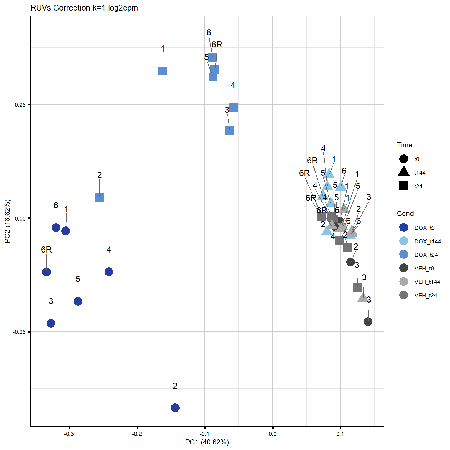
| Version | Author | Date |
|---|---|---|
| a967d53 | emmapfort | 2025-12-09 |
#save for figure generation

# save_plot(plot = fig2a,
#           filename = "Fig2A_PCA_6x8_EMP",
#           folder = output_folder,
#           width = 6,
#           height = 8)
Differential Expression Analysis - RUVs Corrected
#Perform Differential Expression Analysis with k = 1 RUVs Correction
#same DGEList object as before
dge <- readRDS("data/DE/dge_matrix.RDS")
Metadata_2 <- readRDS("data/QC/Metadata_2_norep_update.RDS")
x_norep <- readRDS("data/DE/x_norep.RDS")

#check normalization factors from TMM normalization of LIBRARIES
dge$samples
group lib.size norm.factors
87-1_DOX_24 DOX_t0 19935097 1.0526605
87-1_DMSO_24 VEH_t0 21302879 0.9773889
87-1_DOX_24+24 DOX_t24 25636959 1.0751043
87-1_DMSO_24+24 VEH_t24 26319662 0.9940323
87-1_DOX_24+144 DOX_t144 23463426 0.9003102
87-1_DMSO_24+144 VEH_t144 25840938 0.9888449
78-1_DOX_24 DOX_t0 23085807 0.7676077
78-1_DMSO_24 VEH_t0 25610495 1.0077383
78-1_DOX_24+24 DOX_t24 18083930 1.1682704
78-1_DMSO_24+24 VEH_t24 24331177 0.9906872
78-1_DOX_24+144 DOX_t144 19754391 0.9941834
78-1_DMSO_24+144 VEH_t144 22641509 1.0010734
75-1_DOX_24 DOX_t0 20583626 1.0676786
75-1_DMSO_24 VEH_t0 28166198 1.0031906
75-1_DOX_24+24 DOX_t24 25831427 1.1530208
75-1_DMSO_24+24 VEH_t24 26081158 1.0058953
75-1_DOX_24+144 DOX_t144 24659898 0.9261599
75-1_DMSO_24+144 VEH_t144 25412931 0.9703454
84-1_DOX_24 DOX_t0 23393931 0.9745263
84-1_DMSO_24 VEH_t0 22853195 0.9565797
84-1_DOX_24+24 DOX_t24 23846995 1.1659432
84-1_DMSO_24+24 VEH_t24 21299355 0.9649641
84-1_DOX_24+144 DOX_t144 18222568 0.9913625
84-1_DMSO_24+144 VEH_t144 28115884 0.9653464
17-3_DOX_24 DOX_t0 22518848 0.9766893
17-3_DMSO_24 VEH_t0 24589534 0.9612345
17-3_DOX_24+24 DOX_t24 24797547 1.1703079
17-3_DMSO_24+24 VEH_t24 25977536 0.9509690
17-3_DOX_24+144 DOX_t144 27447106 0.9422729
17-3_DMSO_24+144 VEH_t144 24893583 0.9356377
90-1_DOX_24 DOX_t0 25187428 1.0311957
90-1_DMSO_24 VEH_t0 25630519 1.0283437
90-1_DOX_24+24 DOX_t24 26138399 1.1183471
90-1_DMSO_24+24 VEH_t24 24430396 0.9988688
90-1_DOX_24+144 DOX_t144 23323463 0.9496884
90-1_DMSO_24+144 VEH_t144 25424152 0.9872926#read in my covariate information RUV_1 dataframe + remove 6R
RUV_df_rm1 <- readRDS("data/DE/RUV_df_rm1.RDS")
#filter out 6R for DE analysis
RUV_1_df_filt <- RUV_df_rm1[!grepl("6R$", rownames(RUV_df_rm1)), , drop = FALSE]
Metadata_2$W_1 <- RUV_1_df_filt$W_1
#now ensure that RUV_1 has the right number of cols after removing rep
length(RUV_1_df_filt$W_1)[1] 36#36
#now make this into a list
RUV_1_DE <- RUV_1_df_filt$W_1
# saveRDS(RUV_1_DE, "data/DE/RUV_1_DE.RDS")
#create my design matrix for DE + RUVs covariate k=1
design1 <- model.matrix(~0 + RUV_1_DE + Metadata_2$Condition)
colnames(design1) <- gsub("Metadata_2\\$Condition", "", colnames(design1))
#take care that the matrix automatically sorts cols alphabetically
#run duplicate correlation for individual effect
corfit1 <- duplicateCorrelation(object = dge$counts, design = design1, block = Metadata_2$Ind)
#voom transformation and plot
v1 <- voom(dge, design1, block = Metadata_2$Ind, correlation = corfit1$consensus.correlation, plot = TRUE)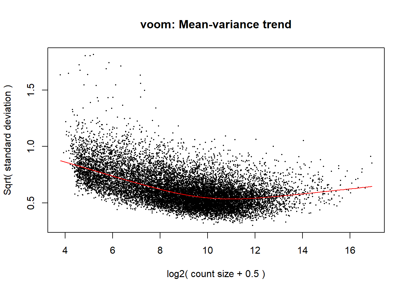
| Version | Author | Date |
|---|---|---|
| a967d53 | emmapfort | 2025-12-09 |
#fit my linear model
fit1 <- lmFit(v1, design1, block = Metadata_2$Ind, correlation = corfit1$consensus.correlation)

#make my contrast matrix to compare across tx and veh
contrast_matrix_RUV <- makeContrasts(
  V.D24T = DOX_t0 - VEH_t0,
  V.D24R = DOX_t24 - VEH_t24,
  V.D144R = DOX_t144 - VEH_t144,
  RUV_1_24T = RUV_1_DE - VEH_t0,
  RUV_1_24R = RUV_1_DE - VEH_t24,
  RUV_1_144R = RUV_1_DE - VEH_t144,
  levels = design1
)

#apply these contrasts to compare DOX to DMSO VEH
fit_RUV <- contrasts.fit(fit1, contrast_matrix_RUV)
fit_RUV <- eBayes(fit_RUV)

#plot the mean-variance trend
plotSA(fit_RUV, main = "Mean-Variance Trend, RUVs k=1")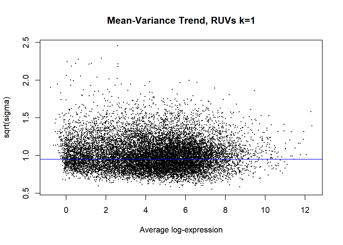
| Version | Author | Date |
|---|---|---|
| a967d53 | emmapfort | 2025-12-09 |
#look at the summary of your results
##this tells you the number of DEGs in each condition
results_summary1 <- decideTests(fit_RUV, adjust.method = "BH", p.value = 0.05)

summary(results_summary1)
V.D24T V.D24R V.D144R RUV_1_24T RUV_1_24R RUV_1_144R
Down 4866 3727 466 10518 10519 10513
NotSig 4899 7107 13659 2905 2899 2889
Up 4554 3485 194 896 901 917# V.D24T V.D24R V.D144R
# Down 4866 3727 466
# NotSig 4899 7107 13659
# Up 4554 3485 194
#compare this to my previous DEGs I found
# summary(results_summary)
# V.D24T V.D24R V.D144R
# Down 4723 3593 359
# NotSig 5076 7151 13810
# Up 4520 3575 150
#overall, there are more DEGs found after RUVs k=1 correction
#this was an expected result as it increases tx effect w/ correctionToptables
##Generate Toptables RUVs
# Generate Top Table for Specific Comparisons
x <- readRDS("data/DE/x_dge_counts_allind_updated.RDS")

Toptable_V.D24T_k1 <- topTable(fit = fit_RUV, coef = "V.D24T", number = nrow(x), adjust.method = "BH", p.value = 1, sort.by = "none")
# write.csv(Toptable_V.D24T_k1, "data/DE/Toptable_V.D24T_k1.csv")

Toptable_V.D24R_k1 <- topTable(fit = fit_RUV, coef = "V.D24R", number = nrow(x), adjust.method = "BH", p.value = 1, sort.by = "none")
# write.csv(Toptable_V.D24R_k1, "data/DE/Toptable_V.D24R_k1.csv")

Toptable_V.D144R_k1 <- topTable(fit = fit_RUV, coef = "V.D144R", number = nrow(x), adjust.method = "BH", p.value = 1, sort.by = "none")
# write.csv(Toptable_V.D144R_k1, "data/DE/Toptable_V.D144R_k1.csv")

# save all of these toptables as R objects
# saveRDS(list(
#   V.D24T_k1 = Toptable_V.D24T_k1,
#   V.D24R_k1 = Toptable_V.D24R_k1,
#   V.D144R_k1 = Toptable_V.D144R_k1
# ), file = "data/DE/Toptable_list_RUVk1.RDS")

# Toptable_list_RUVk1 <- readRDS("data/DE/Toptable_list_RUVk1.RDS")

#################################################################
#this section is commented out since it only needs to run once
#kept the code for posterity

# #I want to add the hgnc symbols to my toptables as well
# ####D24T####
# #load in data
# sample_toptab_24T <- read_csv("C:/Users/emmap/RDirectory/Recovery_RNAseq/Recovery_5FU/data/new/DEGs/Toptable_V.D24T_k1.csv", show_col_types = FALSE)
# # ----------------- Ensure Entrez_ID is Present and in Character Format -----------------
# # Check column names
# print(colnames(sample_toptab_24T))
# # Rename if needed (adjust if the column name is not exactly 'Entrez_ID')
# colnames(sample_toptab_24T)[1] <- "Entrez_ID"
# # Convert Entrez_ID to character
# sample_toptab_24T <- sample_toptab_24T %>%
#   mutate(Entrez_ID = as.character(Entrez_ID))
# # ----------------- Map Entrez_ID to Gene Symbol -----------------
# gene_symbols1 <- AnnotationDbi::select(
#   org.Hs.eg.db,
#   keys = sample_toptab_24T$Entrez_ID,
#   columns = c("SYMBOL"),
#   keytype = "ENTREZID"
# )
# # ----------------- Join Back to Main Data -----------------
# Toptable_RUV_24T <- left_join(sample_toptab_24T, gene_symbols1, by = c("Entrez_ID" = "ENTREZID"))
# Toptable_RUV_24T %>% column_to_rownames(., var = "Entrez_ID")
# # ----------------- Save Annotated Output -----------------
# write_csv(Toptable_RUV_24T, "data/DE/Toptable_RUV_24T.csv")
#
# Toptable_RUV_24T <- read.csv("data/DE/Toptable_RUV_24T.csv")
# #now do this again for my other two toptables
#
# ####24R####
# #load in data
# sample_toptab_24R <- read_csv("C:/Users/emmap/RDirectory/Recovery_RNAseq/Recovery_5FU/data/new/DEGs/Toptable_V.D24R_k1.csv", show_col_types = FALSE)
# # ----------------- Ensure Entrez_ID is Present and in Character Format -----------------
# # Check column names
# print(colnames(sample_toptab_24R))
# # Rename if needed (adjust if the column name is not exactly 'Entrez_ID')
# colnames(sample_toptab_24R)[1] <- "Entrez_ID"
# # Convert Entrez_ID to character
# sample_toptab_24R <- sample_toptab_24R %>%
# mutate(Entrez_ID = as.character(Entrez_ID))
# ----------------- Map Entrez_ID to Gene Symbol -----------------
# gene_symbols2 <- AnnotationDbi::select(
#   org.Hs.eg.db,
#   keys = sample_toptab_24R$Entrez_ID,
#   columns = c("SYMBOL"),
#   keytype = "ENTREZID"
# )
# # ----------------- Join Back to Main Data -----------------
# Toptable_RUV_24R <- left_join(sample_toptab_24R, gene_symbols2, by = c("Entrez_ID" = "ENTREZID"))
# Toptable_RUV_24R %>% column_to_rownames(., var = "Entrez_ID")
# # ----------------- Save Annotated Output -----------------
# #I'll make these symbols into rownames later for my volcano plots
# write_csv(Toptable_RUV_24R, "data/DE/Toptable_RUV_24R.csv")
#

# Toptable_RUV_24R <- read.csv("data/DE/Toptable_RUV_24R.csv")
#
# ####D144R####
# #load in data
# sample_toptab_144R <- read_csv("C:/Users/emmap/RDirectory/Recovery_RNAseq/Recovery_5FU/data/new/DEGs/Toptable_V.D144R_k1.csv", show_col_types = FALSE)
# # ----------------- Ensure Entrez_ID is Present and in Character Format -----------------
# # Check column names
# print(colnames(sample_toptab_144R))
# # Rename if needed (adjust if the column name is not exactly 'Entrez_ID')
# colnames(sample_toptab_144R)[1] <- "Entrez_ID"
# # Convert Entrez_ID to character
# sample_toptab_144R <- sample_toptab_144R %>%
#   mutate(Entrez_ID = as.character(Entrez_ID))
# # ----------------- Map Entrez_ID to Gene Symbol -----------------
# gene_symbols3 <- AnnotationDbi::select(
#   org.Hs.eg.db,
#   keys = sample_toptab_144R$Entrez_ID,
#   columns = c("SYMBOL"),
#   keytype = "ENTREZID"
# )
# # ----------------- Join Back to Main Data -----------------
# Toptable_RUV_144R <- left_join(sample_toptab_144R, gene_symbols3, by = c("Entrez_ID" = "ENTREZID"))
# Toptable_RUV_144R %>% column_to_rownames(., var = "Entrez_ID")
# # ----------------- Save Annotated Output -----------------
# #I'll make these symbols into rownames later for my volcano plots
# write_csv(Toptable_RUV_144R, "data/DE/Toptable_RUV_144R.csv")
#
# write.csv(Toptable_RUV_24T, "data/DE/Toptable_RUV_24T_final.csv")
# write.csv(Toptable_RUV_24R, "data/DE/Toptable_RUV_24R_final.csv")
# write.csv(Toptable_RUV_144R, "data/DE/Toptable_RUV_144R_final.csv")

Toptable_RUV_24T <- read_csv("data/DE/Toptable_RUV_24T_final.csv",
                             col_select = -1)
Toptable_RUV_24R <- read_csv("data/DE/Toptable_RUV_24R_final.csv",
                             col_select = -1)
Toptable_RUV_144R <- read_csv("data/DE/Toptable_RUV_144R_final.csv",
                              col_select = -1)

# save all of these toptables as R objects
# saveRDS(list(
#   V.D24T_RUV = Toptable_RUV_24T,
#   V.D24R_RUV = Toptable_RUV_24R,
#   V.D144R_RUV = Toptable_RUV_144R
# ), file = "data/DE/Toptable_list_RUVk1_Symbols.RDS")

Toptable_list_RUVk1_symbols <- readRDS("data/DE/Toptable_list_RUVk1_Symbols.RDS")
#Figure 2B - Barplot of DEG Percentages
###Proportion of DEGs in Gene Set RUVs corrected
#check the proportion of my genes in my gene set that are DEGs by timepoint

#make this into a pie chart or a bar graph
#read in my full gene set
filcpm_matrix <- readRDS("data/QC/filcpm_final_matrix_newind.RDS")
all_genes <- rownames(filcpm_matrix)

#convert Entrez_ID to Gene Symbols
all_genes_set <- mapIds(org.Hs.eg.db,
                        keys = all_genes,
                        column = "SYMBOL",
                        keytype = "ENTREZID",
                        multiVals = "first")

# Load DEGs Data (replaced with new set)
DOX_t0 <- read_csv("data/DE/Toptable_RUV_24T_final.csv",
                   col_select = -1)
DOX_t24 <- read_csv("data/DE/Toptable_RUV_24R_final.csv",
                    col_select = -1)
DOX_t144 <- read_csv("data/DE/Toptable_RUV_144R_final.csv",
                     col_select = -1)

# Extract Significant DEGs (change names to timepoint)
DEG_t0_RUV <- DOX_t0$Entrez_ID[DOX_t0$adj.P.Val < 0.05]
DEG_t24_RUV <- DOX_t24$Entrez_ID[DOX_t24$adj.P.Val < 0.05]
DEG_t144_RUV <- DOX_t144$Entrez_ID[DOX_t144$adj.P.Val < 0.05]

# saveRDS(DEG_t0_RUV, "data/DE/DEGs_sig_list_24T_RUVs_set.RDS")
# saveRDS(DEG_t24_RUV, "data/DE/DEGs_sig_list_24R_RUVs_set.RDS")
# saveRDS(DEG_t144_RUV, "data/DE/DEGs_sig_list_144R_RUVs_set.RDS")

#make a list of all of my significant DEGs
timepoint_DEGs_RUV <- list(
  "24T" = DEG_t0_RUV,
  "24R" = DEG_t24_RUV,
  "144R" = DEG_t144_RUV
)

# Function to compute proportions
get_proportions_degs <- function(degs, total_genes) {
  deg_count <- length(degs)
  non_deg_count <- total_genes - deg_count
  data.frame(
    Category = c("DEGs", "Non-DEGs"),
    Count = c(deg_count, non_deg_count),
    Proportion = c(deg_count / total_genes, non_deg_count / total_genes)
  )
}

# Compute proportions for each timepoint
prop_t0 <- get_proportions_degs(DEG_t0_RUV, length(all_genes_set))
prop_t24 <- get_proportions_degs(DEG_t24_RUV, length(all_genes_set))
prop_t144 <- get_proportions_degs(DEG_t144_RUV, length(all_genes_set))

# Combine for bar plot
prop_bar <- rbind(
  cbind(Timepoint = "t0", prop_t0),
  cbind(Timepoint = "t24", prop_t24),
  cbind(Timepoint = "t144", prop_t144)
)

#pie chart for t0
ggplot(prop_t0, aes(x = "", y = Count, fill = Category)) +
  geom_bar(stat = "identity", width = 1) +
  coord_polar("y") +
  labs(title = "DEGs vs Non-DEGs (t0)") +
  theme_void()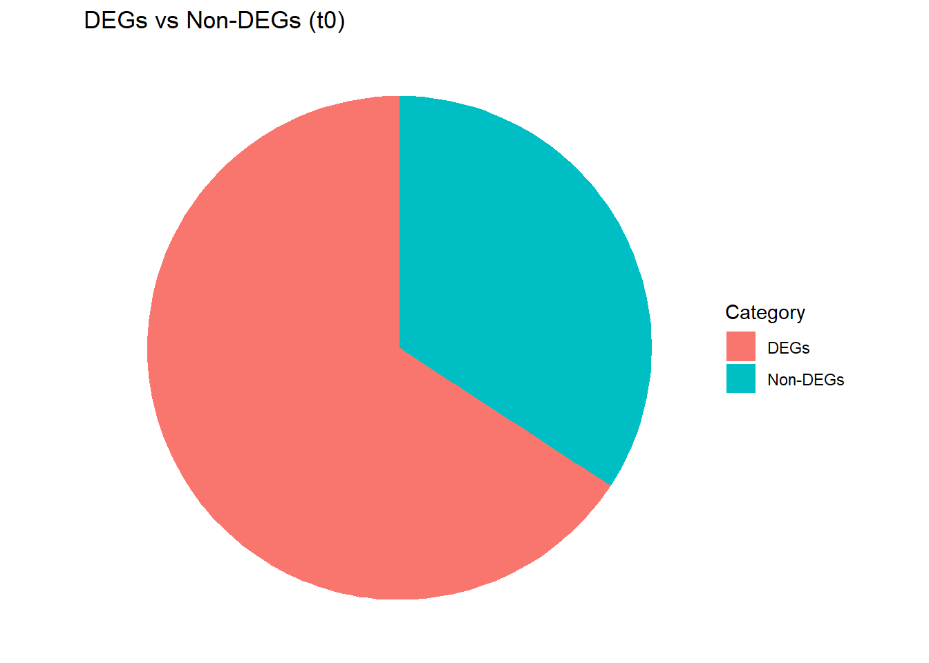
| Version | Author | Date |
|---|---|---|
| a967d53 | emmapfort | 2025-12-09 |
#pie chart for t24
ggplot(prop_t24, aes(x = "", y = Count, fill = Category)) +
  geom_bar(stat = "identity", width = 1) +
  coord_polar("y") +
  labs(title = "DEGs vs Non-DEGs (t24)") +
  theme_void()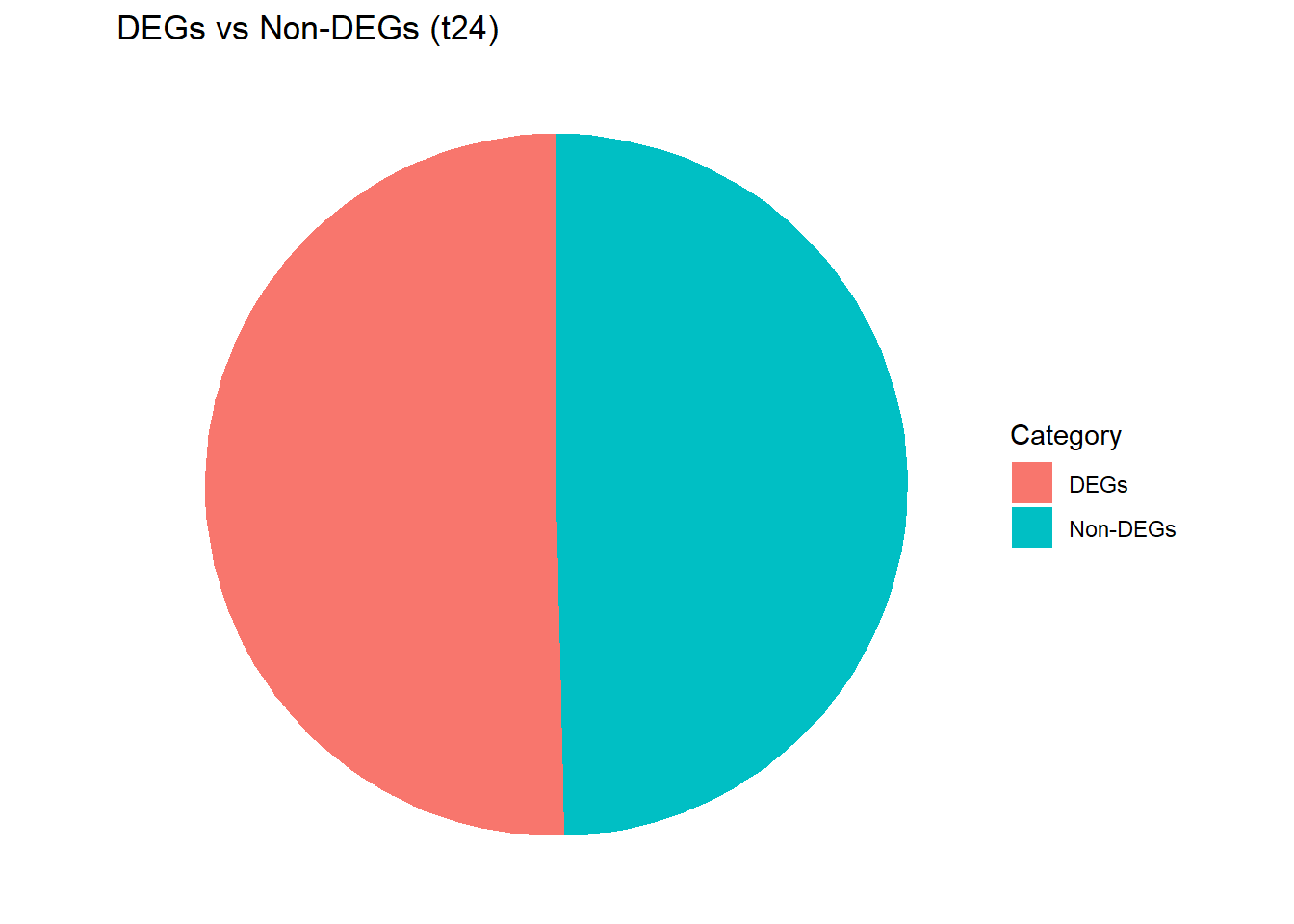
| Version | Author | Date |
|---|---|---|
| a967d53 | emmapfort | 2025-12-09 |
#pie chart for t144
ggplot(prop_t144, aes(x = "", y = Count, fill = Category)) +
  geom_bar(stat = "identity", width = 1) +
  coord_polar("y") +
  labs(title = "DEGs vs Non-DEGs (t144)") +
  theme_void()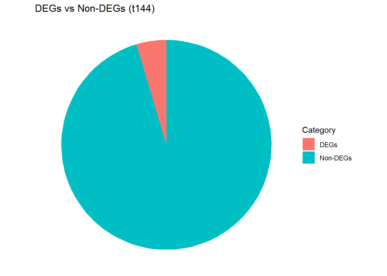
| Version | Author | Date |
|---|---|---|
| a967d53 | emmapfort | 2025-12-09 |
#put the desired colors here for your pie charts
degs_prop_colors <- c("DEGs" = "red", "Non-DEGs" = "blue")

#labels for percentage based on proportion
prop_t0$Label <- paste0(round(prop_t0$Proportion * 100, 1), "")
prop_t24$Label <- paste0(round(prop_t24$Proportion * 100, 1), "")
prop_t144$Label <- paste0(round(prop_t144$Proportion * 100, 1), "")

#create each plot and assign to variables
plot_t0 <- ggplot(prop_t0, aes(x = "", y = Count, fill = Category)) +
  geom_bar(stat = "identity", width = 1) +
  coord_polar("y") +
  geom_text(aes(label = Label),
            position = position_stack(vjust = 0.6),
            color = "white",
            size = 4) +
  scale_fill_manual(values = degs_prop_colors) +
  labs(title = "t0") +
  theme_void()

plot_t24 <- ggplot(prop_t24, aes(x = "", y = Count, fill = Category)) +
  geom_bar(stat = "identity", width = 1) +
  coord_polar("y") +
  geom_text(aes(label = Label),
            position = position_stack(vjust = 0.6),
            color = "white",
            size = 4) +
  scale_fill_manual(values = degs_prop_colors) +
  labs(title = "t24") +
  theme_void()

plot_t144 <- ggplot(prop_t144, aes(x = "", y = Count, fill = Category)) +
  geom_bar(stat = "identity", width = 1) +
  coord_polar("y") +
  geom_text(aes(label = Label),
            position = position_stack(vjust = 0.6),
            color = "white",
            size = 4) +
  scale_fill_manual(values = degs_prop_colors) +
  labs(title = "t144") +
  theme_void()

#combine all three pie charts in a row
combined_prop_degs_plots <-
  plot_t0 +
  plot_t24 +
  plot_t144 +
  plot_layout(ncol = 3, nrow = 1, guides = "collect") +
  plot_annotation(title = "Proportion of DEGs vs Non-DEGs")

#show the combined pie chart plot
combined_prop_degs_plots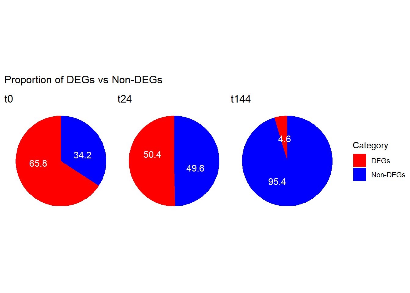
| Version | Author | Date |
|---|---|---|
| a967d53 | emmapfort | 2025-12-09 |
#combine all three pie charts in a column
combined_prop_degs_plots_col <-
  plot_t0 +
  plot_t24 +
  plot_t144 +
  plot_layout(ncol = 1, nrow = 3, guides = "collect") +
  plot_annotation(title = "Proportion of DEGs vs Non-DEGs")

#show the combined pie chart plot in 1 column
combined_prop_degs_plots_col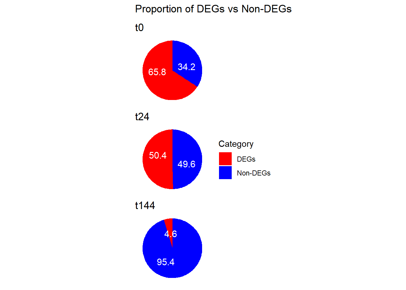
| Version | Author | Date |
|---|---|---|
| a967d53 | emmapfort | 2025-12-09 |
####proportion bar plots####
#first factor the timepoints so that they are in the right order
prop_bar$Timepoint <- factor(prop_bar$Timepoint,
                             levels = c("t0", "t24", "t144"))

#percentage labels
prop_bar$Label <- paste0(round(prop_bar$Proportion * 100, 1), "")

#plot the bar plot
barplot_deg_perc <- ggplot(prop_bar, aes(x = Timepoint,
                     y = Proportion,
                     fill = Category)) +
  geom_bar(stat = "identity",
           position = "fill") +
  geom_text(aes(label = Label),
            position = position_fill(vjust = 0.5),
            color = "white",
            size = 4) +
  scale_fill_manual(values = degs_prop_colors) +
  labs(title = "Percentage of DEGs vs nonDEGs by Timepoint",
       y = "Percentage of DEGs (%)",
       x = "") +
  scale_y_continuous(labels = c(0, 25, 50, 75, 100)) +
  theme_custom()

print(barplot_deg_perc)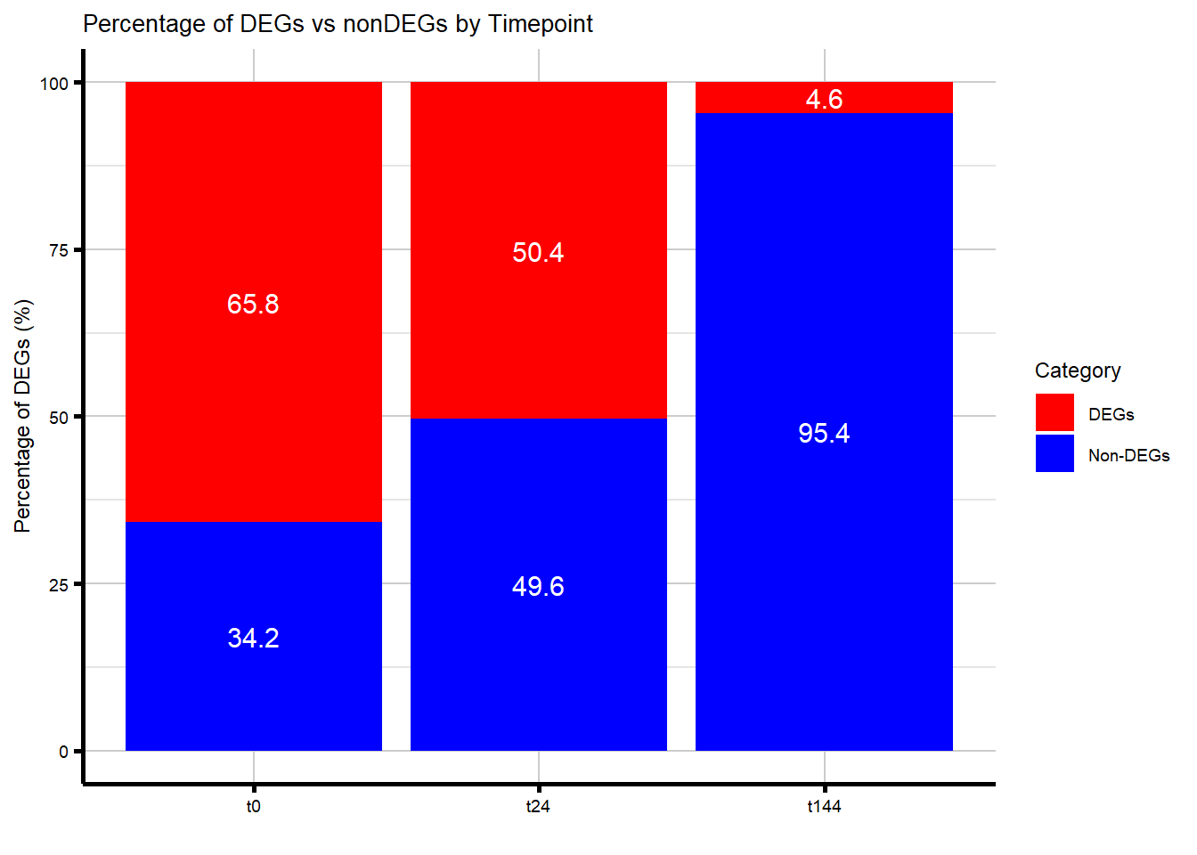
| Version | Author | Date |
|---|---|---|
| a967d53 | emmapfort | 2025-12-09 |
#save this barplot
# save_plot(
# plot = barplot_deg_perc,
# filename = "DEGvsnonDEG_Barplot_update_EMP",
# folder = output_folder
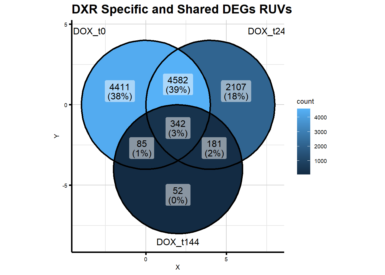
# )Figure 2C - Venn Diagram of DEG Overlap
##Venn Diagrams of DEG Overlap after RUVs Correction k=1
#plot a venn diagram with all of your conditions from your toptables

# Load DEGs Data (already read in above)
# DOX_t0 <- read_csv("data/DE/Toptable_RUV_24T_final.csv",
#                    col_select = -1)
# DOX_t24 <- read_csv("data/DE/Toptable_RUV_24R_final.csv",
#                     col_select = -1)
# DOX_t144 <- read_csv("data/DE/Toptable_RUV_144R_final.csv",
#                      col_select = -1)

# Extract Significant DEGs (change names to timepoint)
# DEG_t0_RUV <- DOX_t0$Entrez_ID[DOX_t0$adj.P.Val < 0.05]
# DEG_t24_RUV <- DOX_t24$Entrez_ID[DOX_t24$adj.P.Val < 0.05]
# DEG_t144_RUV <- DOX_t144$Entrez_ID[DOX_t144$adj.P.Val < 0.05]

venn_test_RUV <- list(DEG_t0_RUV, DEG_t24_RUV, DEG_t144_RUV)

ggVennDiagram(
  venn_test_RUV,
  category.names = c("DOX_t0", "DOX_t24", "DOX_t144")
) + ggtitle("DXR Specific and Shared DEGs RUVs")+
  theme_custom() +
  theme(
    plot.title = element_text(size = 16, face = "bold"),  # Increase title size
    text = element_text(size = 16)  # Increase text size globally
  )
| Version | Author | Date |
|---|---|---|
| a967d53 | emmapfort | 2025-12-09 |
####I want to make this proportional
#use the eulerr package to do so

venn_prop_RUV <- euler(list(
  "t0" = DEG_t0_RUV,
  "t24" = DEG_t24_RUV,
  "t144" = DEG_t144_RUV
))

plot(venn_prop_RUV,
     fills = list(fill = c("#263CA5", "#5B8FD1", "#89C5E5"),
                  alpha = 1),
     labels = list(font = 4),
     quantities = list(cex = 0.75),
     main = "")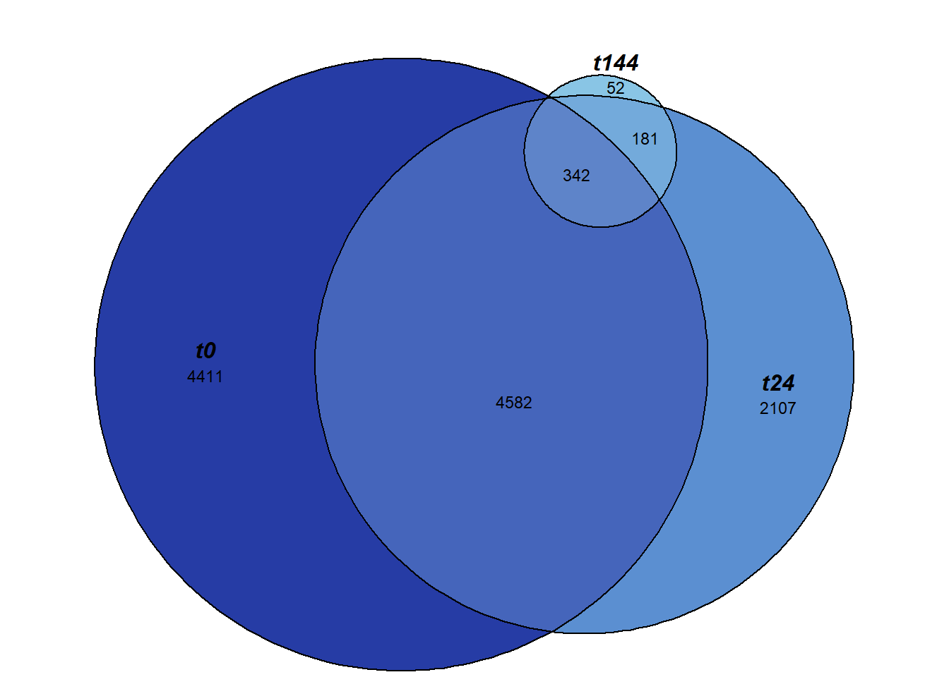
| Version | Author | Date |
|---|---|---|
| a967d53 | emmapfort | 2025-12-09 |
Load in DEGs
#Load DEGs Data
#make a list of all of the genes in this set so I can plot the logFC in other sets

# Load DEGs Data (already read in above)
# DOX_t0 <- read_csv("data/DE/Toptable_RUV_24T_final.csv",
#                    col_select = -1)
# DOX_t24 <- read_csv("data/DE/Toptable_RUV_24R_final.csv",
#                     col_select = -1)
# DOX_t144 <- read_csv("data/DE/Toptable_RUV_144R_final.csv",
#                      col_select = -1)

DOX_24T_R <- read_csv("data/DE/Toptable_RUV_24T.csv")
DOX_24R_R <- read_csv("data/DE/Toptable_RUV_24R_final.csv")
DOX_144R_R <- read_csv("data/DE/Toptable_RUV_144R_final.csv")

#plot those full gene sets in logFC
D24T_DEGs_R <- DOX_t0$Entrez_ID[DOX_t0$adj.P.Val < 0.05]
length(D24T_DEGs_R)
[1] 9420#9420 DEGs
D24R_DEGs_R <- DOX_t24$Entrez_ID[DOX_t24$adj.P.Val < 0.05]
length(D24R_DEGs_R)[1] 7212#7168 DEGs
D144R_DEGs_R <- DOX_t144$Entrez_ID[DOX_t144$adj.P.Val < 0.05]
length(D144R_DEGs_R)[1] 660#660 DEGs
#now that I have the full list of genes, I want to plot the logFC across conditions
#Combine the toptables I have from pairwise analysis into a single dataframe
d24_toptable_dxr_1 <- Toptable_RUV_24T %>%
mutate(Time = "t0")
d24r_toptable_dxr_1 <- Toptable_RUV_24R %>%
mutate(Time = "t24")
d144r_toptable_dxr_1 <- Toptable_RUV_144R %>%
mutate(Time = "t144")
combined_toptables_dxr_RUV <- bind_rows(
d24_toptable_dxr_1,
d24r_toptable_dxr_1,
d144r_toptable_dxr_1)
# saveRDS(combined_toptables_dxr_RUV, "data/DE/combined_toptables_dxr_RUV.RDS")Figure 2D - Scatterplots logFC Timepoint Comparisons
# Define the timepoints from your data
timepoints <- c("t0", "t24", "t144")

comparison_order <- c("t0 vs t24", "t24 vs t144", "t0 vs t144")

# Make all pairwise combinations
pairs_df <- t(combn(timepoints, 2)) %>%
  as.data.frame(stringsAsFactors = FALSE) %>%
  setNames(c("time_x", "time_y"))

logFC_wide_RUV <- combined_toptables_dxr_RUV %>%
  mutate(absFC = abs(logFC)) %>%
  dplyr::select(Entrez_ID, Time, logFC) %>%
  pivot_wider(names_from = Time, values_from = logFC) %>%
  drop_na() %>%
  column_to_rownames("Entrez_ID")

# Function to prepare scatter data for each pair
prepare_pair_data <- function(time_x, time_y, df) {
  rho <- cor(df[[time_x]], df[[time_y]], method = "spearman")
  df %>%
    mutate(
      x_val = .data[[time_x]],
      y_val = .data[[time_y]],
      comparison = paste0(time_x, " vs ", time_y),
      rho_label = paste0("rho = ", round(rho, 2)),
      x_lab = paste0("log2FC", time_x),
      y_lab = paste0("log2FC", time_y)
    )
}

comparison_colors <- c(
  "t0 vs t24"  = "#4167BD",
  "t24 vs t144" = "#72AEE0",
  "t0 vs t144" = "#5780C5"
)

# Build combined plotting dataset
scatter_df <- map2_df(pairs_df$time_x, pairs_df$time_y,
                      ~prepare_pair_data(.x, .y, logFC_wide_RUV)) %>%
  mutate(comparison = factor(comparison, levels = comparison_order))

facet_labels <- scatter_df %>%
  distinct(comparison, x_lab, y_lab) %>%
  mutate(label = paste0(comparison, "\n", x_lab, " | ", y_lab)) %>%
  dplyr::select(comparison, label) %>%
  deframe()

#split data by comparison
split_data <- split(scatter_df, scatter_df$comparison)

make_scatter <- function(df_sub) {
  comp <- df_sub$comparison[1]
  ggplot(df_sub, aes(x = x_val, y = y_val)) +
    geom_point_rast(alpha = 0.5, raster.dpi = 300, color = comparison_colors[comp]) +
    geom_smooth(method = "lm", se = FALSE, linetype = "dashed", color = "black") +
    geom_text(
      data = df_sub %>% distinct(comparison, rho_label),
      aes(x = -Inf, y = Inf, label = rho_label),
    inherit.aes = FALSE,
    hjust = -0.1, vjust = 1.5,
    size = 4
  ) +
    coord_fixed(xlim = c(-9,9), ylim = c(-9,9), ratio = 1) +
    labs(
      x = unique(df_sub$x_lab),
      y = unique(df_sub$y_lab)
    ) +
    theme_custom() +
    theme(
      axis.line = element_line(linewidth = 1,
                               color = "black"),
      axis.ticks.length = unit(0.05, "in"),
      axis.text = element_text(color = "black"),
      panel.background = element_blank(),
      panel.border = element_blank(),
      legend.position = "none"
    )
}

#make plot
plot_list <- lapply(split_data, make_scatter)

#wrap all three together to get the final plot
scatterplot_fig2d_wide <- wrap_plots(plot_list, ncol  = length(plot_list))
scatterplot_fig2d_tall <- wrap_plots(plot_list, nrow = length(plot_list))
scatterplot_fig2d_wide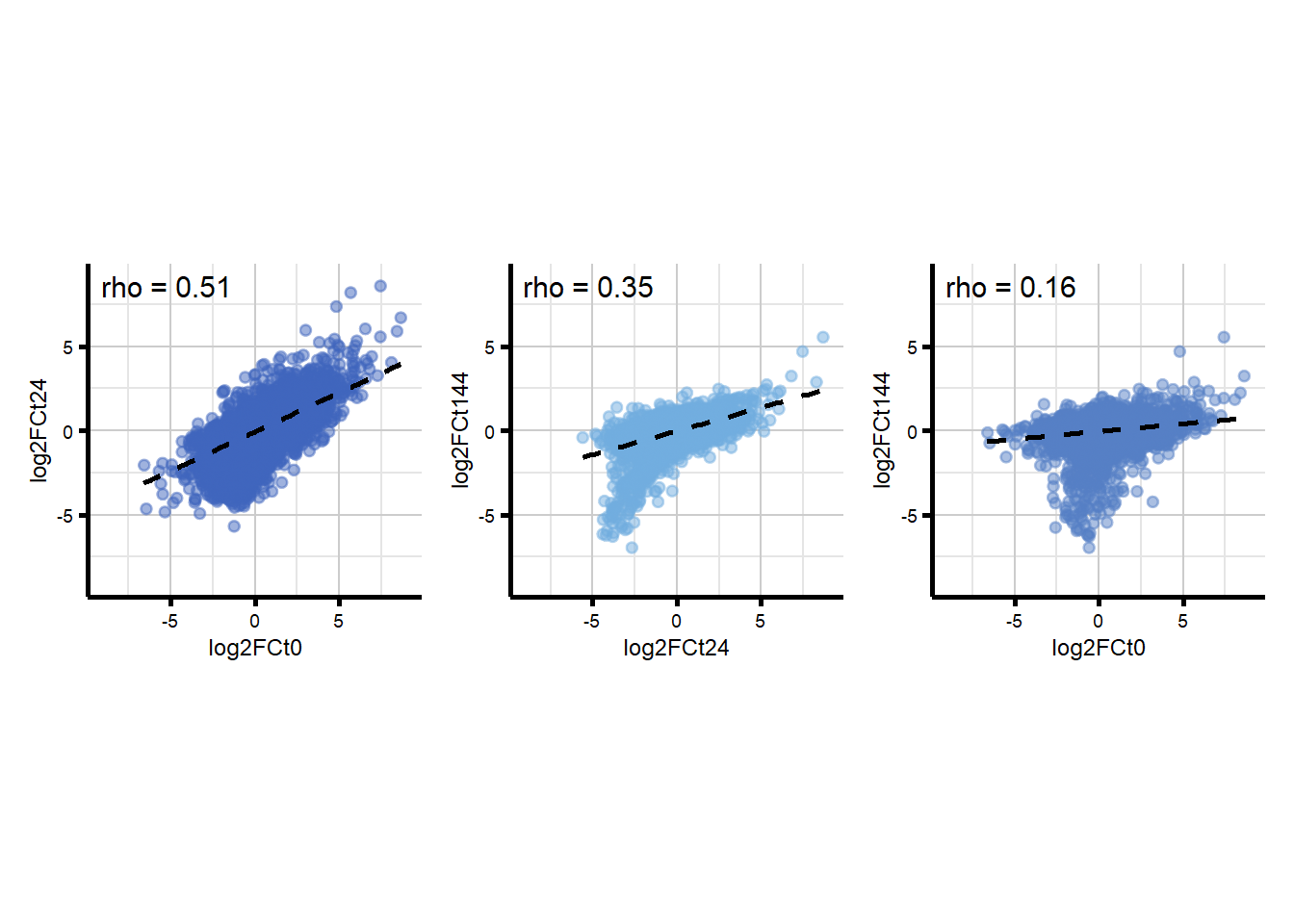
| Version | Author | Date |
|---|---|---|
| a967d53 | emmapfort | 2025-12-09 |
scatterplot_fig2d_tall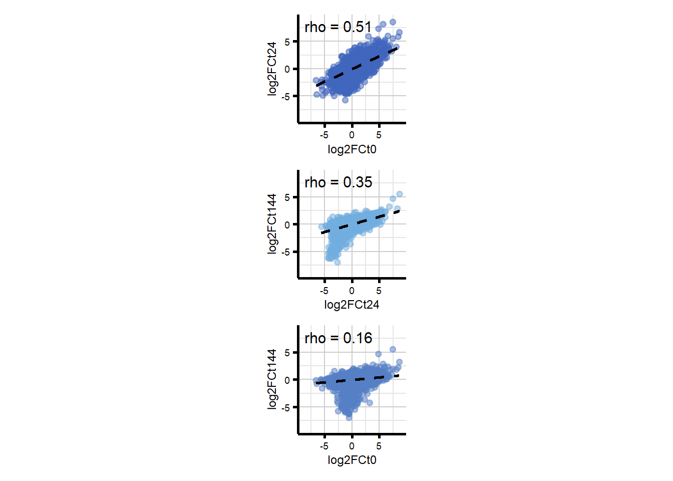
| Version | Author | Date |
|---|---|---|
| a967d53 | emmapfort | 2025-12-09 |
#save plot to a pdf and to a png
# ggsave("Fig2D_Scatterplot_fixedlims_EMP_251121.pdf", scatterplot_fig2d_wide, width = 8, height = 6, device = cairo_pdf, path = "C:/Users/emmap/OneDrive/Desktop/DXR Manuscript Materials/Fig pdfs")
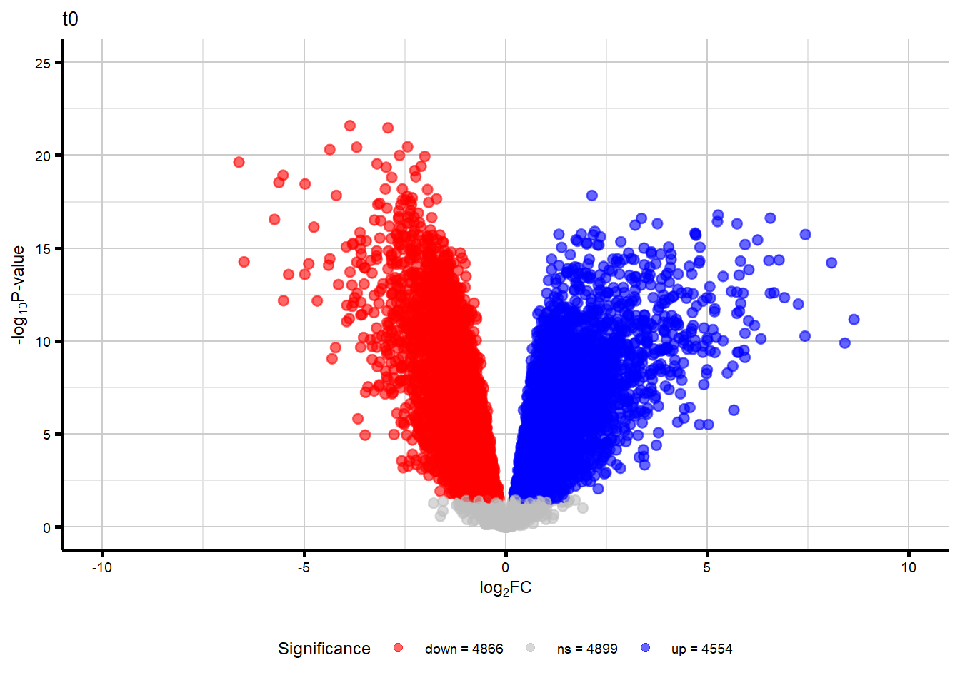
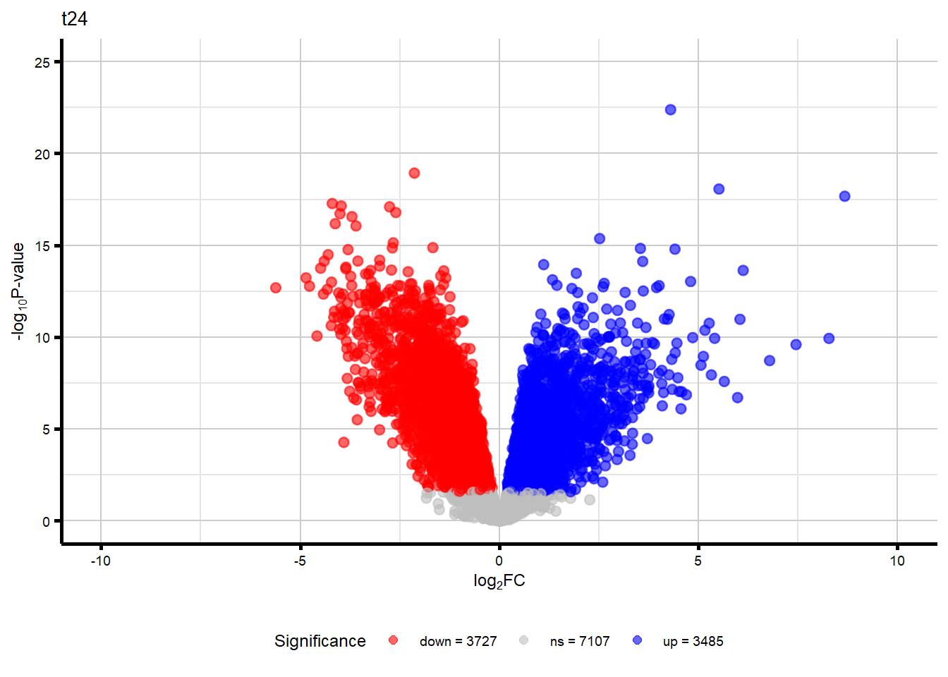
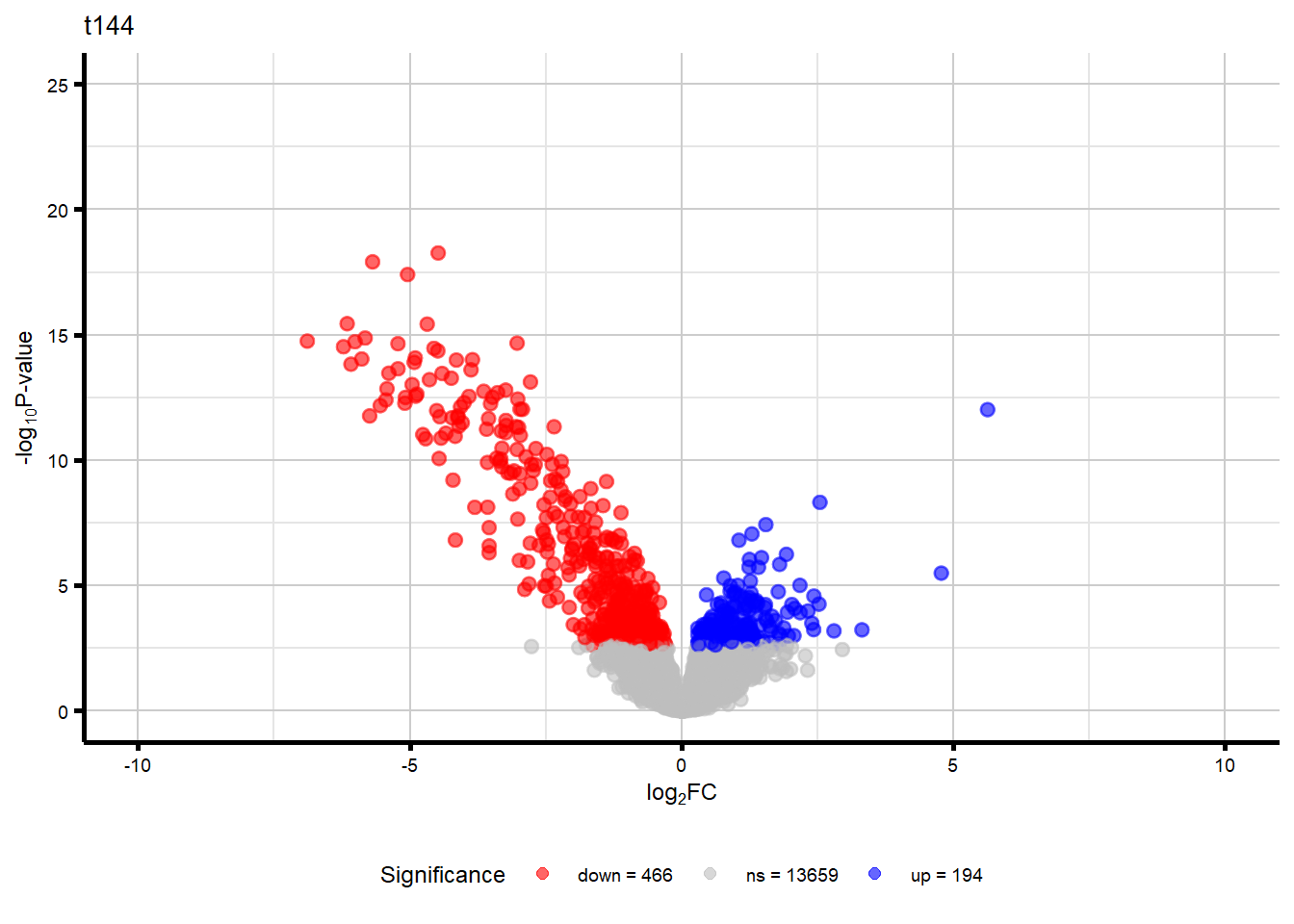
# ggsave("Fig2D_Scatterplot_fixedlims_EMP_251121.png", scatterplot_fig2d_wide, width = 12, height = 4, dpi = 300, type = "cairo", path = "C:/Users/emmap/OneDrive/Desktop/DXR Manuscript Materials/Fig pdfs")Supplementary Figure 4 - Volcano Plots of RUVs DEGs
#make a function to generate volcano plots + add gene numbers
#ensure the gene symbols are in a col so I can plot names of top 15
generate_volcano_plot_RUV <- function(toptable, title) {

  #make significance labels
  toptable$Significance <- "Not Significant"
  toptable$Significance[toptable$logFC > 0 & toptable$adj.P.Val < 0.05] <- "Upregulated"
  toptable$Significance[toptable$logFC < 0 & toptable$adj.P.Val < 0.05] <- "Downregulated"

  #enforce correct factor order
  toptable$Significance <- factor(
    toptable$Significance,
    levels = c("Downregulated", "Not Significant", "Upregulated")
  )

  #add number of genes for each significance label
  upgenes <- toptable %>%
    filter(Significance == "Upregulated") %>%
    nrow()
  nsgenes <- toptable %>%
    filter(Significance == "Not Significant") %>%
    nrow()
  downgenes <- toptable %>%
    filter(Significance == "Downregulated") %>%
    nrow()

  #FIX: correct legend labels
  legend_lab <- c(
    "Upregulated" = paste0("up = ", upgenes),
    "Not Significant" = paste0("ns = ", nsgenes),
    "Downregulated" = paste0("down = ", downgenes)
  )

  #FIX: correct legend colors
  legend_col <- c(
    "Upregulated" = "blue",
    "Not Significant" = "gray",
    "Downregulated" = "red"
  )

  #generate volcano plot w/ legend
  p <- ggplot(toptable, aes(x = logFC,
                            y = -log10(P.Value),
                            color = Significance)) +
    geom_point_rast(alpha = 0.6, size = 2) +  #rasterize
    scale_color_manual(values = legend_col,
                       labels = legend_lab) +
    xlim(-10, 10) +
    ylim(0, 25) +
    labs(title = title,
         x = expression("log"[2]*"FC"),
         y = expression("-log"[10]*"P-value")) +
    theme_custom() +
    theme(legend.position = "bottom")

  return(p)
}


#generate volcano plots across each comparison
volcano_plots_RUV <- list(
  "Volcano_Supp4_1_EMP" = generate_volcano_plot_RUV(Toptable_RUV_24T, "t0"),
  "Volcano_Supp4_2_EMP" = generate_volcano_plot_RUV(Toptable_RUV_24R, "t24"),
  "Volcano_Supp4_3_EMP" = generate_volcano_plot_RUV(Toptable_RUV_144R, "t144")
)

# Display each volcano plot
for (plot_name in names(volcano_plots_RUV)) {
  print(volcano_plots_RUV[[plot_name]])
}
#save all volcano plots
for (plot_name in names(volcano_plots_RUV)) {
  save_plot(
    filename = paste0(plot_name, "_EMP.pdf"),
    plot = volcano_plots_RUV[[plot_name]],
    height = 4,
    width = 4,
    folder = output_folder
  )
}
sessionInfo()R version 4.4.2 (2024-10-31 ucrt)
Platform: x86_64-w64-mingw32/x64
Running under: Windows 11 x64 (build 22000)
Matrix products: default
locale:
[1] LC_COLLATE=English_United States.utf8
[2] LC_CTYPE=English_United States.utf8
[3] LC_MONETARY=English_United States.utf8
[4] LC_NUMERIC=C
[5] LC_TIME=English_United States.utf8
time zone: America/Chicago
tzcode source: internal
attached base packages:
[1] stats4 stats graphics grDevices utils datasets methods
[8] base
other attached packages:
[1] ggrastr_1.0.2 ggVennDiagram_1.5.2
[3] org.Hs.eg.db_3.20.0 AnnotationDbi_1.68.0
[5] eulerr_7.0.2 patchwork_1.3.0
[7] RUVSeq_1.40.0 edgeR_4.4.0
[9] limma_3.62.1 EDASeq_2.40.0
[11] ShortRead_1.64.0 GenomicAlignments_1.42.0
[13] SummarizedExperiment_1.36.0 MatrixGenerics_1.18.1
[15] matrixStats_1.5.0 Rsamtools_2.22.0
[17] GenomicRanges_1.58.0 Biostrings_2.74.0
[19] GenomeInfoDb_1.42.3 XVector_0.46.0
[21] IRanges_2.40.0 S4Vectors_0.44.0
[23] BiocParallel_1.40.0 Biobase_2.66.0
[25] BiocGenerics_0.52.0 ggfortify_0.4.17
[27] ggrepel_0.9.6 readxl_1.4.5
[29] lubridate_1.9.4 forcats_1.0.0
[31] stringr_1.5.1 dplyr_1.1.4
[33] purrr_1.0.4 readr_2.1.5
[35] tidyr_1.3.1 tibble_3.2.1
[37] ggplot2_3.5.2 tidyverse_2.0.0
[39] workflowr_1.7.1
loaded via a namespace (and not attached):
[1] splines_4.4.2 later_1.4.2 BiocIO_1.16.0
[4] bitops_1.0-9 filelock_1.0.3 R.oo_1.27.1
[7] cellranger_1.1.0 polyclip_1.10-7 XML_3.99-0.18
[10] lifecycle_1.0.4 httr2_1.1.2 pwalign_1.2.0
[13] rprojroot_2.0.4 processx_3.8.6 lattice_0.22-6
[16] vroom_1.6.5 MASS_7.3-61 magrittr_2.0.3
[19] sass_0.4.10 rmarkdown_2.29 jquerylib_0.1.4
[22] yaml_2.3.10 httpuv_1.6.16 DBI_1.2.3
[25] RColorBrewer_1.1-3 abind_1.4-8 zlibbioc_1.52.0
[28] R.utils_2.13.0 RCurl_1.98-1.17 rappdirs_0.3.3
[31] git2r_0.36.2 GenomeInfoDbData_1.2.13 codetools_0.2-20
[34] DelayedArray_0.32.0 xml2_1.3.8 tidyselect_1.2.1
[37] UCSC.utils_1.2.0 farver_2.1.2 BiocFileCache_2.14.0
[40] jsonlite_2.0.0 systemfonts_1.2.2 polylabelr_0.3.0
[43] tools_4.4.2 progress_1.2.3 ragg_1.4.0
[46] Rcpp_1.0.14 glue_1.8.0 gridExtra_2.3
[49] SparseArray_1.6.0 xfun_0.52 mgcv_1.9-1
[52] withr_3.0.2 fastmap_1.2.0 latticeExtra_0.6-30
[55] callr_3.7.6 digest_0.6.37 timechange_0.3.0
[58] R6_2.6.1 textshaping_1.0.1 colorspace_2.1-1
[61] Cairo_1.6-5 jpeg_0.1-11 biomaRt_2.62.1
[64] RSQLite_2.3.9 R.methodsS3_1.8.2 generics_0.1.4
[67] rtracklayer_1.66.0 prettyunits_1.2.0 httr_1.4.7
[70] S4Arrays_1.6.0 whisker_0.4.1 pkgconfig_2.0.3
[73] gtable_0.3.6 blob_1.2.4 hwriter_1.3.2.1
[76] htmltools_0.5.8.1 scales_1.4.0 png_0.1-8
[79] knitr_1.50 rstudioapi_0.17.1 tzdb_0.5.0
[82] rjson_0.2.23 nlme_3.1-166 curl_6.0.1
[85] cachem_1.1.0 parallel_4.4.2 vipor_0.4.7
[88] restfulr_0.0.15 pillar_1.10.2 grid_4.4.2
[91] vctrs_0.6.5 promises_1.3.2 dbplyr_2.5.0
[94] beeswarm_0.4.0 evaluate_1.0.3 GenomicFeatures_1.58.0
[97] cli_3.6.3 locfit_1.5-9.12 compiler_4.4.2
[100] rlang_1.1.6 crayon_1.5.3 labeling_0.4.3
[103] interp_1.1-6 aroma.light_3.36.0 ps_1.9.1
[106] getPass_0.2-4 fs_1.6.6 ggbeeswarm_0.7.2
[109] stringi_1.8.7 deldir_2.0-4 Matrix_1.7-1
[112] hms_1.1.3 bit64_4.5.2 KEGGREST_1.46.0
[115] statmod_1.5.0 memoise_2.0.1 bslib_0.9.0
[118] bit_4.5.0