Figure 1 Analysis
Last updated: 2026-01-06
Checks: 7 0
Knit directory: DXR_website/
This reproducible R Markdown analysis was created with workflowr (version 1.7.1). The Checks tab describes the reproducibility checks that were applied when the results were created. The Past versions tab lists the development history.
Great! Since the R Markdown file has been committed to the Git repository, you know the exact version of the code that produced these results.
Great job! The global environment was empty. Objects defined in the global environment can affect the analysis in your R Markdown file in unknown ways. For reproduciblity it’s best to always run the code in an empty environment.
The command set.seed(20251201) was run prior to running
the code in the R Markdown file. Setting a seed ensures that any results
that rely on randomness, e.g. subsampling or permutations, are
reproducible.
Great job! Recording the operating system, R version, and package versions is critical for reproducibility.
Nice! There were no cached chunks for this analysis, so you can be confident that you successfully produced the results during this run.
Great job! Using relative paths to the files within your workflowr project makes it easier to run your code on other machines.
Great! You are using Git for version control. Tracking code development and connecting the code version to the results is critical for reproducibility.
The results in this page were generated with repository version cd535e9. See the Past versions tab to see a history of the changes made to the R Markdown and HTML files.
Note that you need to be careful to ensure that all relevant files for
the analysis have been committed to Git prior to generating the results
(you can use wflow_publish or
wflow_git_commit). workflowr only checks the R Markdown
file, but you know if there are other scripts or data files that it
depends on. Below is the status of the Git repository when the results
were generated:
Ignored files:
    Ignored:    .Rhistory
    Ignored:    .Rproj.user/
    Ignored:    DXR_website/data/
    Ignored:    code/Flow_Purity_Stressor_Boxplots_EMP_250226.R
    Ignored:    data/CDKN1A_geneplot_Dox.RDS
    Ignored:    data/Cormotif_dox.RDS
    Ignored:    data/Cormotif_prob_gene_list.RDS
    Ignored:    data/Cormotif_prob_gene_list_doxonly.RDS
    Ignored:    data/Counts_RNA_EMPfortmiller.txt
    Ignored:    data/DMSO_TNN13_plot.RDS
    Ignored:    data/DOX_TNN13_plot.RDS
    Ignored:    data/DOXgeneplots.RDS
    Ignored:    data/ExpressionMatrix_EMP.csv
    Ignored:    data/Ind1_DOX_Spearman_plot.RDS
    Ignored:    data/Ind6REP_Spearman_list.csv
    Ignored:    data/Ind6REP_Spearman_plot.RDS
    Ignored:    data/Ind6REP_Spearman_set.csv
    Ignored:    data/Ind6_Spearman_plot.RDS
    Ignored:    data/MDM2_geneplot_Dox.RDS
    Ignored:    data/Master_summary_75-1_EMP_250811_final.csv
    Ignored:    data/Master_summary_87-1_EMP_250811_final.csv
    Ignored:    data/Metadata.csv
    Ignored:    data/Metadata_2_norep_update.RDS
    Ignored:    data/Metadata_update.csv
    Ignored:    data/QC/
    Ignored:    data/Recovery_flow_purity.csv
    Ignored:    data/SIRT1_geneplot_Dox.RDS
    Ignored:    data/Sample_annotated.csv
    Ignored:    data/SpearmanHeatmapMatrix_EMP
    Ignored:    data/VolcanoPlot_D144R_original_EMP_250623.png
    Ignored:    data/VolcanoPlot_D24R_original_EMP_250623.png
    Ignored:    data/VolcanoPlot_D24T_original_EMP_250623.png
    Ignored:    data/annot_dox.RDS
    Ignored:    data/annot_list_hm.csv
    Ignored:    data/cormotif_dxr_1.RDS
    Ignored:    data/cormotif_dxr_2.RDS
    Ignored:    data/counts/
    Ignored:    data/counts_DE_df_dox.RDS
    Ignored:    data/counts_DE_raw_data.RDS
    Ignored:    data/counts_raw_filt.RDS
    Ignored:    data/counts_raw_matrix.RDS
    Ignored:    data/counts_raw_matrix_EMP_250514.csv
    Ignored:    data/d24_Spearman_plot.RDS
    Ignored:    data/dge_calc_dxr.RDS
    Ignored:    data/dge_calc_matrix.RDS
    Ignored:    data/ensembl_backup_dox.RDS
    Ignored:    data/fC_AllCounts.RDS
    Ignored:    data/fC_DOXCounts.RDS
    Ignored:    data/featureCounts_Concat_Matrix_DOXSamples_EMP_250430.csv
    Ignored:    data/featureCounts_DOXdata_updatedind.RDS
    Ignored:    data/filcpm_colnames_matrix.csv
    Ignored:    data/filcpm_matrix.csv
    Ignored:    data/filt_gene_list_dox.RDS
    Ignored:    data/filter_gene_list_final.RDS
    Ignored:    data/final_data/
    Ignored:    data/gene_clustlike_motif.RDS
    Ignored:    data/gene_postprob_motif.RDS
    Ignored:    data/genedf_dxr.RDS
    Ignored:    data/genematrix_dox.RDS
    Ignored:    data/genematrix_dxr.RDS
    Ignored:    data/heartgenes.csv
    Ignored:    data/heartgenes_dox.csv
    Ignored:    data/image_intensity_stats_all_conditions.csv
    Ignored:    data/image_level_stats_all_conditions.csv
    Ignored:    data/image_level_summary_yH2AX_quant.csv
    Ignored:    data/ind_num_dox.RDS
    Ignored:    data/ind_num_dxr.RDS
    Ignored:    data/initial_cormotif.RDS
    Ignored:    data/initial_cormotif_dox.RDS
    Ignored:    data/low_nuclei_samples.csv
    Ignored:    data/low_veh_samples.csv
    Ignored:    data/new/
    Ignored:    data/new_cormotif_dox.RDS
    Ignored:    data/perc_mean_all_10X.png
    Ignored:    data/perc_mean_all_20X.png
    Ignored:    data/perc_mean_all_40X.png
    Ignored:    data/perc_mean_consistent_10X.png
    Ignored:    data/perc_mean_consistent_20X.png
    Ignored:    data/perc_mean_consistent_40X.png
    Ignored:    data/perc_median_all_10X.png
    Ignored:    data/perc_median_all_20X.png
    Ignored:    data/perc_median_all_40X.png
    Ignored:    data/perc_median_consistent_10X.png
    Ignored:    data/perc_median_consistent_20X.png
    Ignored:    data/perc_median_consistent_40X.png
    Ignored:    data/plot_leg_d.RDS
    Ignored:    data/plot_leg_d_horizontal.RDS
    Ignored:    data/plot_leg_d_vertical.RDS
    Ignored:    data/plot_theme_custom.RDS
    Ignored:    data/process_gene_data_funct.RDS
    Ignored:    data/raw_mean_all_10X.png
    Ignored:    data/raw_mean_all_20X.png
    Ignored:    data/raw_mean_all_40X.png
    Ignored:    data/raw_mean_consistent_10X.png
    Ignored:    data/raw_mean_consistent_20X.png
    Ignored:    data/raw_mean_consistent_40X.png
    Ignored:    data/raw_median_all_10X.png
    Ignored:    data/raw_median_all_20X.png
    Ignored:    data/raw_median_all_40X.png
    Ignored:    data/raw_median_consistent_10X.png
    Ignored:    data/raw_median_consistent_20X.png
    Ignored:    data/raw_median_consistent_40X.png
    Ignored:    data/ruv/
    Ignored:    data/summary_all_IF_ROI.RDS
    Ignored:    data/tableED_GOBP.RDS
    Ignored:    data/tableESR_GOBP_postprob.RDS
    Ignored:    data/tableLD_GOBP.RDS
    Ignored:    data/tableLR_GOBP_postprob.RDS
    Ignored:    data/tableNR_GOBP.RDS
    Ignored:    data/tableNR_GOBP_postprob.RDS
    Ignored:    data/table_incsus_genes_GOBP_RUV.RDS
    Ignored:    data/table_motif1_GOBP_d.RDS
    Ignored:    data/table_motif1_genes_GOBP.RDS
    Ignored:    data/table_motif2_GOBP_d.RDS
    Ignored:    data/table_motif3_genes_GOBP.RDS
    Ignored:    data/thing.R
    Ignored:    data/top.table_V.D144r_dox.RDS
    Ignored:    data/top.table_V.D24_dox.RDS
    Ignored:    data/top.table_V.D24r_dox.RDS
    Ignored:    data/yH2AX_75-1_EMP_250811.csv
    Ignored:    data/yH2AX_87-1_EMP_250811.csv
    Ignored:    data/yH2AX_Boxplots_MeanIntensity_10X_EMP_250811.png
    Ignored:    data/yH2AX_Boxplots_MeanIntensity_10X_NormtoMax_EMP_250811.png
    Ignored:    data/yH2AX_Boxplots_MeanIntensity_20X_EMP_250811.png
    Ignored:    data/yH2AX_Boxplots_MeanIntensity_20X_NormtoMax_EMP_250811.png
    Ignored:    data/yH2AX_Boxplots_MedianIntensity_10X_NormtoMax_EMP_250811.png
    Ignored:    data/yH2AX_Boxplots_MedianIntensity_20X_NormtoMax_EMP_250811.png
    Ignored:    data/yH2AX_Boxplots_MedianIntensity_NormtoMax_EMP_250811.png
    Ignored:    data/yH2AX_Boxplots_Quant_10X_EMP_250817.png
    Ignored:    data/yH2AX_Boxplots_Quant_20X_EMP_250817.png
    Ignored:    data/yh2ax_all_df_EMP_250812.csv

Unstaged changes:
    Modified:   analysis/DXR_Project_Analysis.Rmd
Note that any generated files, e.g. HTML, png, CSS, etc., are not included in this status report because it is ok for generated content to have uncommitted changes.
These are the previous versions of the repository in which changes were
made to the R Markdown (DXR_website/analysis/Figure1.Rmd)
and HTML (DXR_website/docs/Figure1.html) files. If you’ve
configured a remote Git repository (see ?wflow_git_remote),
click on the hyperlinks in the table below to view the files as they
were in that past version.
| File | Version | Author | Date | Message |
|---|---|---|---|---|
| Rmd | cd535e9 | emmapfort | 2026-01-06 | Final Website Touches 01/06/25 EMP |
| html | 7f22593 | emmapfort | 2026-01-05 | Build site. |
| Rmd | 108c3dd | emmapfort | 2025-12-01 | updated new website |
| html | c523397 | emmapfort | 2025-12-01 | Build site. |
| html | 0f7b54c | emmapfort | 2025-12-01 | Build site. |
| Rmd | 099ed2b | emmapfort | 2025-12-01 | New Website Commit |
| Rmd | 9a22c3c | emmapfort | 2025-12-01 | Updated Analysis 12/01/25 |
Libraries
Load necessary libraries for analysis.
library(tidyverse)
library(readxl)
library(readr)
library(drc)
library(scales)
library(RImageJROI) #to read in ROI from ImageJ/Fiji
library(stringr)
library(purrr)
library(rstatix)
library(ggpubr)
Define my custom plot theme
# Define the custom theme
# plot_theme_custom <- function() {
#   theme_minimal() +
#     theme(
#       #line for x and y axis
#       axis.line = element_line(linewidth = 1,
#                                color = "black"),
#
#       #axis ticks only on x and y, length standard
#       axis.ticks.x = element_line(color = "black",
#                                 linewidth = 1),
#       axis.ticks.y = element_line(color = "black",
#                                 linewidth = 1),
#       axis.ticks.length = unit(0.05, "in"),
#
#       #text and font
#       axis.text = element_text(color = "black",
#                                family = "Arial",
#                                size = 7),
#       axis.title = element_text(color = "black",
#                                 family = "Arial",
#                                 size = 9),
#       legend.text = element_text(color = "black",
#                                  family = "Arial",
#                                  size = 7),
#       legend.title = element_text(color = "black",
#                                   family = "Arial",
#                                   size = 9),
#       plot.title = element_text(color = "black",
#                                 family = "Arial",
#                                 size = 10),
#
#       #blank background and border
#       panel.background = element_blank(),
#       panel.border = element_blank(),
#
#       #gridlines for alignment
#       panel.grid.major = element_line(color = "grey80", linewidth = 0.5),  #grey major grid for align in illus
#       panel.grid.minor = element_line(color = "grey90", linewidth = 0.5) #grey minor grid for align in illus
#     )
# }

# saveRDS(plot_theme_custom, "data/plot_theme_custom.RDS")

theme_custom <- readRDS("data/plot_theme_custom.RDS")
Define a function to save plots as .pdf and .png
save_plot <- function(plot, filename,
                      folder = ".",
                      width = 8,
                      height = 6,
                      units = "in",
                      dpi = 300,
                      add_date = TRUE) {
  if (missing(filename)) stop("Please provide a filename (without extension) for the plot.")

  date_str <- if (add_date) paste0("_", format(Sys.Date(), "%y%m%d")) else ""
  pdf_file <- file.path(folder, paste0(filename, date_str, ".pdf"))
  png_file <- file.path(folder, paste0(filename, date_str, ".png"))
  ggsave(filename = pdf_file, plot = plot, device = cairo_pdf, width = width, height = height, units = units, bg = "transparent")
  ggsave(filename = png_file, plot = plot, device = "png", width = width, height = height, units = units, dpi = dpi, bg = "transparent")
  message("Saved plot as Cairo PDF: ", pdf_file)
  message("Saved plot as PNG: ", png_file)
}

output_folder <- "C:/Users/emmap/OneDrive/Desktop/DXR Manuscript Materials/Fig pdfs"


#save plot function created
#to use: just define the plot name, filename_base, width, height
Figure 1A - Experimental Schematic (no code)
This schematic did not require analysis.
Figure 1B - Flow Cytometry Barplot
Data to create Figure 1B.
#Individuals for Flow Cytometry
#1 = 87-1 (F)
#2 = 78-1 (F)
#3 = 75-1 (F)
#4 = 84-1 (M)
#5 = 17-3 (M)
#6 = 90-1 (M)
#6R = 90-1R (M)

ind_col <- list(
  "1" = "#FF9F64",
  "2" = "#78EBDA",
  "3" = "#ADCD77",
  "4" = "#E6CC50",
  "5" = "#A68AC0",
  "6" = "#F16F90",
  "7" = "#C61E4E"
)

#read in csv with flow cytometry information
flow_dxr <- read_csv("C:/Users/emmap/OneDrive/Desktop/Ward Lab/Experiments/DXR Project/Flow/Recovery_flow_purity.csv",
                     show_col_types = FALSE)

# View(flow_dxr)

flow <- flow_dxr %>% column_to_rownames("Line")

#make a barplot

flow_dxr_df <- as.data.frame(flow_dxr)

#Plot
flow_plot_tnnt2 <- ggplot(flow_dxr_df, aes(x = Ind, y = Purity)) +
  geom_bar(stat = "identity",
           fill = ind_col,
           width = 0.3 / (0.3 + 0.02)) +
  scale_y_continuous(limits = c(0, 100),
                     expand = c(0, 0)) +
  scale_x_discrete(expand = expansion(mult = c(0.02, 0.02)))+
  labs(title = "iPSC-CM Purity",
       y = "TNNT2 Expression (%)",
       x = "Individual") +
  theme_custom() +
  theme(strip.text.y = element_text(color = "white"))

print(flow_plot_tnnt2)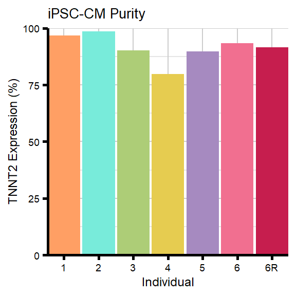
| Version | Author | Date |
|---|---|---|
| 0f7b54c | emmapfort | 2025-12-01 |
# save_plot(
#   plot = flow_plot_tnnt2,
#   filename = "FlowCytometry_TNNT2_withrep_EMP",
#   folder = output_folder,
#   width = 2.8,
#   height = 5.25
# )
Figure 1C - Dose Response Curves
Data for Figure 1C.
AllData <- read_excel("C:/Users/emmap/OneDrive/Desktop/Ward Lab/Experiments/DXR Project/DRCs/5FUProj_DRCTime_78-1_75-1_17-3_EMP_240226.xlsx",
     sheet = "Fin_Sheet_Analysis")
# View(AllData)

Ind2_78_data <- read_excel("C:/Users/emmap/OneDrive/Desktop/Ward Lab/Experiments/DXR Project/DRCs/5FUProj_DRCTime_78-1_75-1_17-3_EMP_240226.xlsx",
     sheet = "Fin_78_Sheet")
# View(Ind2_78_data)

#this is now Individual 2 after reordering individuals earlier - 78-1 F

Ind3_75_data <- read_excel("C:/Users/emmap/OneDrive/Desktop/Ward Lab/Experiments/DXR Project/DRCs/5FUProj_DRCTime_78-1_75-1_17-3_EMP_240226.xlsx",
     sheet = "Fin_75_Sheet")
# View(Ind3_75_data)

#this is now Ind3 since I reordered individuals - 75-1 F

Ind5_17_data <- read_excel("C:/Users/emmap/OneDrive/Desktop/Ward Lab/Experiments/DXR Project/DRCs/5FUProj_DRCTime_78-1_75-1_17-3_EMP_240226.xlsx",
     sheet = "Fin_17_Sheet")
# View(Ind5_17_data)

#this is still ind 5 according to my RNAseq - 17-3 M
Filter for Time and Treatment Groups
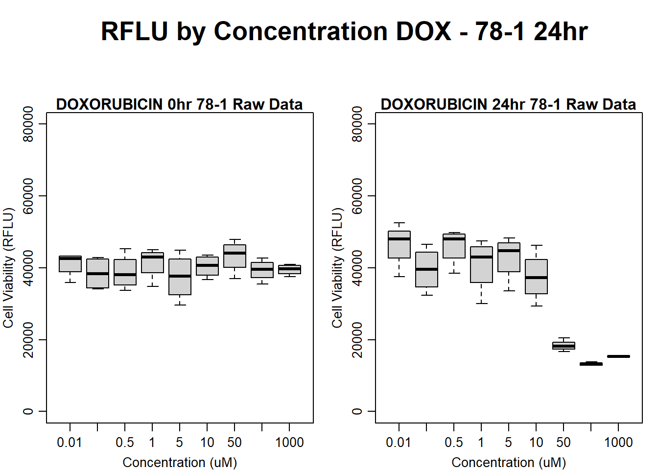
Analysis of Raw Data
#####DOX Samples#####
#dox 78-1 24HR
par(mar = c(3.0, 3.0, 1.2, 1), mgp = c(2, .7, 0))
layout(matrix(c(1, 2, 1, 3), nrow = 2, ncol = 2), heights = c(0.5, 2, 2, 2))
#layout.show(3)
plot.new()
text(0.5,0.5,"RFLU by Concentration DOX - 78-1 24hr",cex = 2,font = 2)

boxplot(dox24hr78$Ind2_78_In ~ dox24hr78$Conc,
        ylim = c(0, 80000),
        ylab = "Cell Viability (RFLU)",
        xlab = "Concentration (uM)",
        main = "DOXORUBICIN 0hr 78-1 Raw Data"
)

boxplot(dox24hr78$Ind2_78_Fin ~ dox24hr78$Conc,
        ylim = c(0,80000),
        ylab = "Cell Viability (RFLU)",
        xlab = "Concentration (uM)",
        main = "DOXORUBICIN 24hr 78-1 Raw Data"
)
| Version | Author | Date |
|---|---|---|
| 0f7b54c | emmapfort | 2025-12-01 |
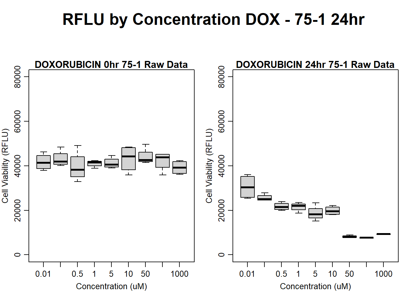
#dox 75-1 24HR
par(mar = c(3.0, 3.0, 1.2, 1), mgp = c(2, .7, 0))
layout(matrix(c(1, 2, 1, 3), nrow = 2, ncol = 2), heights = c(0.5, 2, 2, 2))
#layout.show(3)
plot.new()
text(0.5,0.5,"RFLU by Concentration DOX - 75-1 24hr",cex = 2,font = 2)

boxplot(dox24hr75$Ind1_75_In ~ dox24hr75$Conc,
        ylim = c(0, 80000),
        ylab = "Cell Viability (RFLU)",
        xlab = "Concentration (uM)",
        main = "DOXORUBICIN 0hr 75-1 Raw Data"
)

boxplot(dox24hr75$Ind1_75_Fin ~ dox24hr75$Conc,
        ylim = c(0,80000),
        ylab = "Cell Viability (RFLU)",
        xlab = "Concentration (uM)",
        main = "DOXORUBICIN 24hr 75-1 Raw Data"
)
| Version | Author | Date |
|---|---|---|
| 0f7b54c | emmapfort | 2025-12-01 |
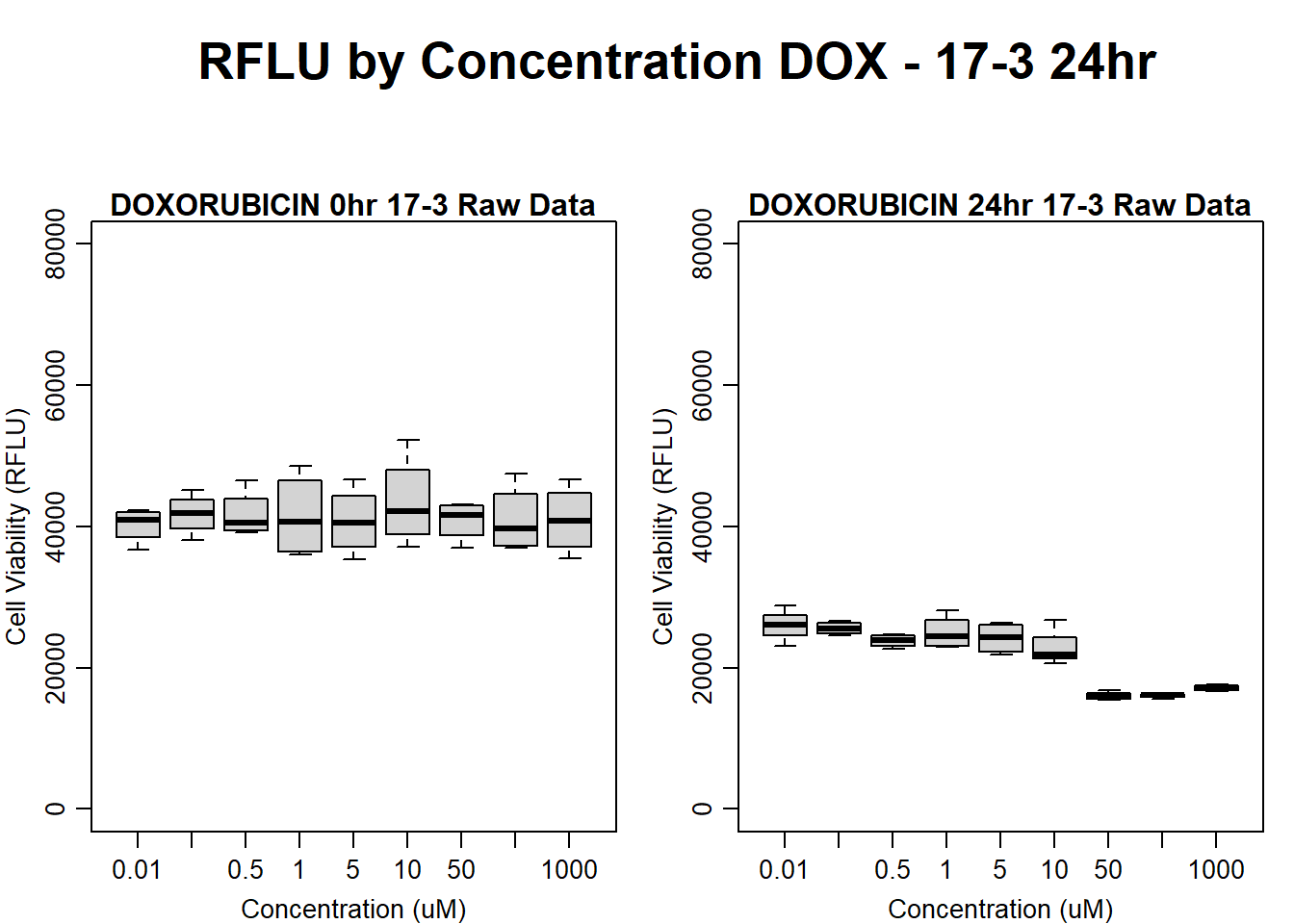
#dox 17-3 24HR
par(mar = c(3.0, 3.0, 1.2, 1), mgp = c(2, .7, 0))
layout(matrix(c(1, 2, 1, 3), nrow = 2, ncol = 2), heights = c(0.5, 2, 2, 2))
#layout.show(3)
plot.new()
text(0.5,0.5,"RFLU by Concentration DOX - 17-3 24hr",cex = 2,font = 2)

boxplot(dox24hr17$Ind3_17_In ~ dox24hr17$Conc,
        ylim = c(0, 80000),
        ylab = "Cell Viability (RFLU)",
        xlab = "Concentration (uM)",
        main = "DOXORUBICIN 0hr 17-3 Raw Data"
)

boxplot(dox24hr17$Ind3_17_Fin ~ dox24hr17$Conc,
        ylim = c(0,80000),
        ylab = "Cell Viability (RFLU)",
        xlab = "Concentration (uM)",
        main = "DOXORUBICIN 24hr 17-3 Raw Data"
)
| Version | Author | Date |
|---|---|---|
| 0f7b54c | emmapfort | 2025-12-01 |
#####DMSO samples#####
#DMSO 78-1 24HR
par(mar = c(3.0, 3.0, 1.2, 1), mgp = c(2, .7, 0))
layout(matrix(c(1, 2, 1, 3), nrow = 2, ncol = 2), heights = c(0.5, 2, 2, 2))
#layout.show(3)
plot.new()
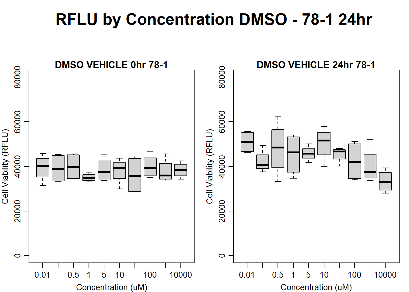
text(0.5,0.5,"RFLU by Concentration DMSO - 78-1 24hr",cex = 2,font = 2)
boxplot(dmso24hr78$Ind2_78_In ~ dmso24hr78$Conc,
ylim = c(0, 80000),
ylab = "Cell Viability (RFLU)",
xlab = "Concentration (uM)",
main = "DMSO VEHICLE 0hr 78-1"
)
boxplot(dmso24hr78$Ind2_78_Fin ~ dmso24hr78$Conc,
ylim = c(0,80000),
ylab = "Cell Viability (RFLU)",
xlab = "Concentration (uM)",
main = "DMSO VEHICLE 24hr 78-1"
)
| Version | Author | Date |
|---|---|---|
| 0f7b54c | emmapfort | 2025-12-01 |
#DMSO 75-1 24HR
par(mar = c(3.0, 3.0, 1.2, 1), mgp = c(2, .7, 0))
layout(matrix(c(1, 2, 1, 3), nrow = 2, ncol = 2), heights = c(0.5, 2, 2, 2))
#layout.show(3)
plot.new()
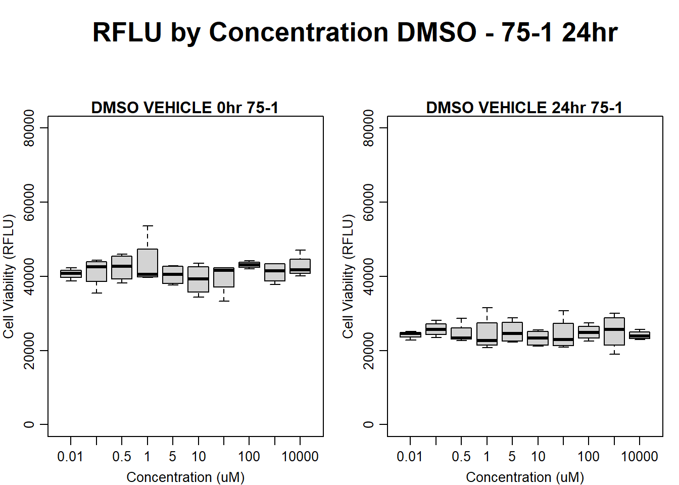
text(0.5,0.5,"RFLU by Concentration DMSO - 75-1 24hr",cex = 2,font = 2)
boxplot(dmso24hr75$Ind1_75_In ~ dmso24hr75$Conc,
ylim = c(0, 80000),
ylab = "Cell Viability (RFLU)",
xlab = "Concentration (uM)",
main = "DMSO VEHICLE 0hr 75-1"
)
boxplot(dmso24hr75$Ind1_75_Fin ~ dmso24hr75$Conc,
ylim = c(0,80000),
ylab = "Cell Viability (RFLU)",
xlab = "Concentration (uM)",
main = "DMSO VEHICLE 24hr 75-1"
)
| Version | Author | Date |
|---|---|---|
| 0f7b54c | emmapfort | 2025-12-01 |
#DMSO 17-3 24HR
par(mar = c(3.0, 3.0, 1.2, 1), mgp = c(2, .7, 0))
layout(matrix(c(1, 2, 1, 3), nrow = 2, ncol = 2), heights = c(0.5, 2, 2, 2))
#layout.show(3)
plot.new()
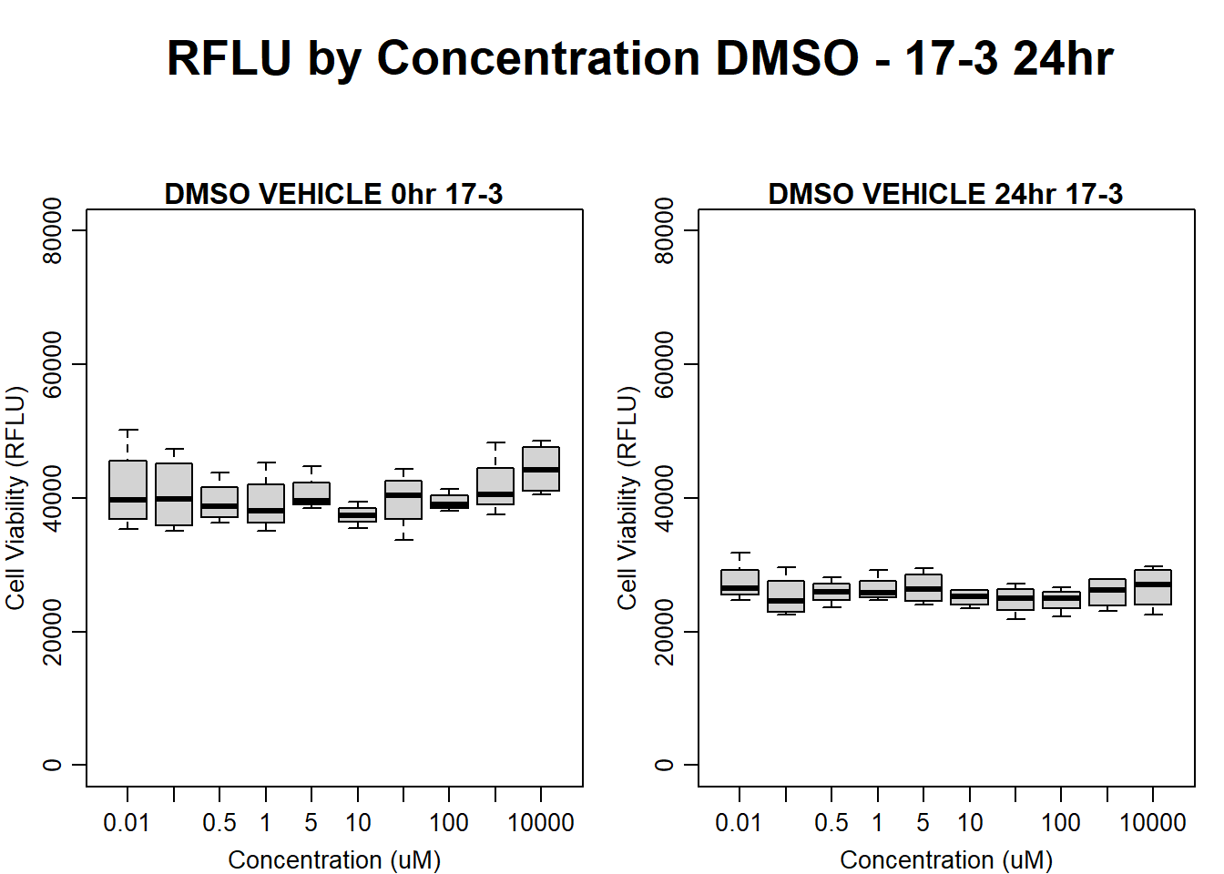
text(0.5,0.5,"RFLU by Concentration DMSO - 17-3 24hr",cex = 2,font = 2)
boxplot(dmso24hr17$Ind3_17_In ~ dmso24hr17$Conc,
ylim = c(0, 80000),
ylab = "Cell Viability (RFLU)",
xlab = "Concentration (uM)",
main = "DMSO VEHICLE 0hr 17-3"
)
boxplot(dmso24hr17$Ind3_17_Fin ~ dmso24hr17$Conc,
ylim = c(0,80000),
ylab = "Cell Viability (RFLU)",
xlab = "Concentration (uM)",
main = "DMSO VEHICLE 24hr 17-3"
)
| Version | Author | Date |
|---|---|---|
| 0f7b54c | emmapfort | 2025-12-01 |
Now that I’ve taken a look at the raw data, let’s look at the analyzed data step by step
The following steps were taken in analysis:
Import raw fluorescence values (RFLU) from platereader, baseline 0hr and final timepoint
Subtract background wells (prestoblue only wells) by plate
Subtract average of empty wells (galactose only, with 50k cells/well) by plate
Divide all values by matched vehicle average (ie DOX 0.01 / DMSO 0.01)
Divide initial 0hr value from final timepoint (24, 48, 72) value
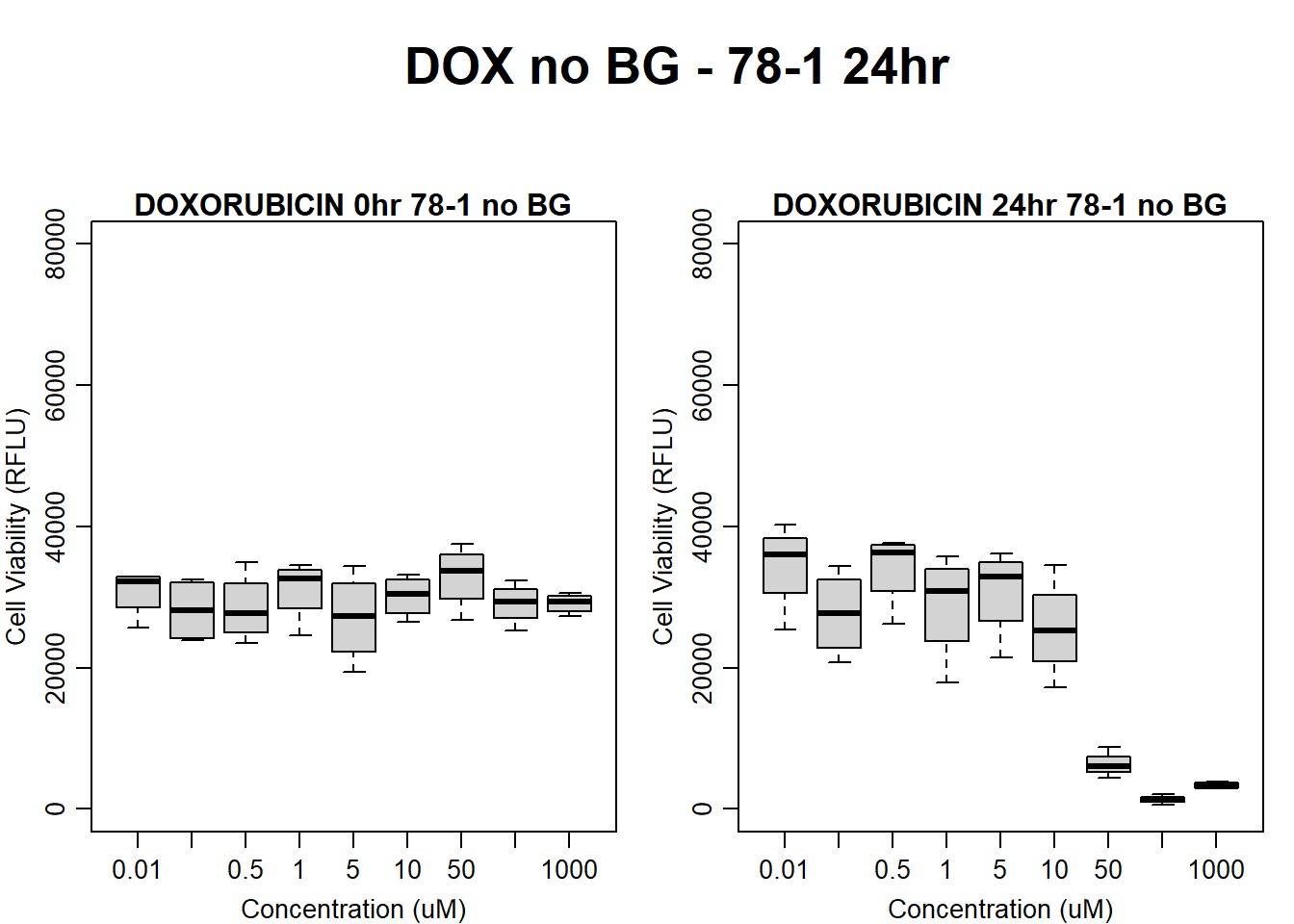
Remove Background Wells
#####DOX Samples#####
#dox 78-1 no BG 24HR
par(mar = c(3.0, 3.0, 1.2, 1), mgp = c(2, .7, 0))
layout(matrix(c(1, 2, 1, 3), nrow = 2, ncol = 2), heights = c(0.5, 2, 2, 2))
#layout.show(3)
plot.new()
text(0.5,0.5,"DOX no BG - 78-1 24hr",cex = 2,font = 2)

boxplot(dox24hr78$Ind2_78_In_noBG ~ dox24hr78$Conc,
        ylim = c(0, 80000),
        ylab = "Cell Viability (RFLU)",
        xlab = "Concentration (uM)",
        main = "DOXORUBICIN 0hr 78-1 no BG"
)

boxplot(dox24hr78$Ind2_78_Fin_noBG ~ dox24hr78$Conc,
        ylim = c(0,80000),
        ylab = "Cell Viability (RFLU)",
        xlab = "Concentration (uM)",
        main = "DOXORUBICIN 24hr 78-1 no BG"
)
| Version | Author | Date |
|---|---|---|
| 0f7b54c | emmapfort | 2025-12-01 |
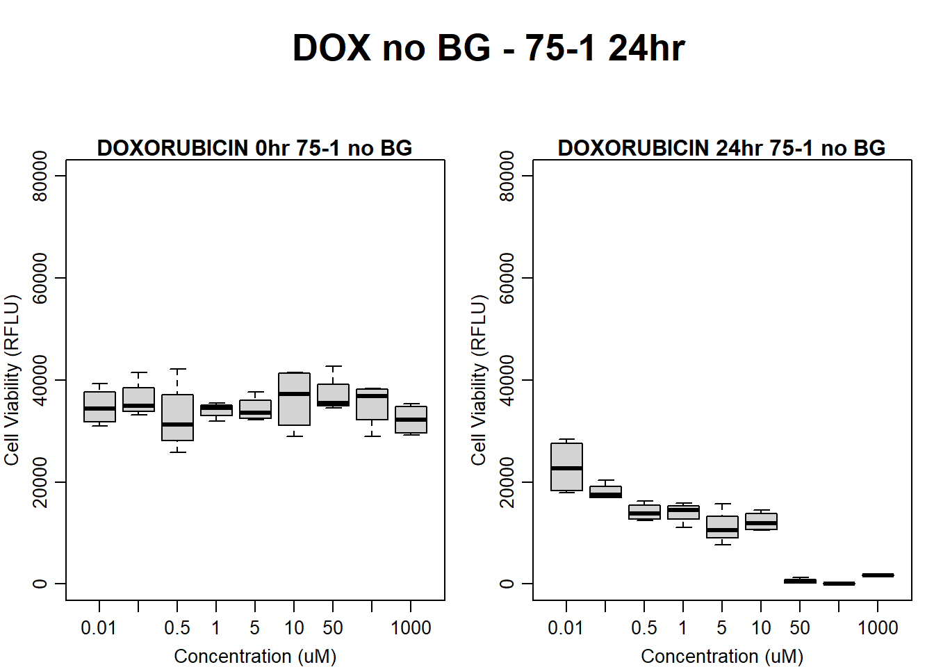
#dox 75-1 24HR
par(mar = c(3.0, 3.0, 1.2, 1), mgp = c(2, .7, 0))
layout(matrix(c(1, 2, 1, 3), nrow = 2, ncol = 2), heights = c(0.5, 2, 2, 2))
#layout.show(3)
plot.new()
text(0.5,0.5,"DOX no BG - 75-1 24hr",cex = 2,font = 2)

boxplot(dox24hr75$Ind1_75_In_noBG ~ dox24hr75$Conc,
        ylim = c(0, 80000),
        ylab = "Cell Viability (RFLU)",
        xlab = "Concentration (uM)",
        main = "DOXORUBICIN 0hr 75-1 no BG"
)

boxplot(dox24hr75$Ind1_75_Fin_noBG ~ dox24hr75$Conc,
        ylim = c(0,80000),
        ylab = "Cell Viability (RFLU)",
        xlab = "Concentration (uM)",
        main = "DOXORUBICIN 24hr 75-1 no BG"
)
| Version | Author | Date |
|---|---|---|
| 0f7b54c | emmapfort | 2025-12-01 |
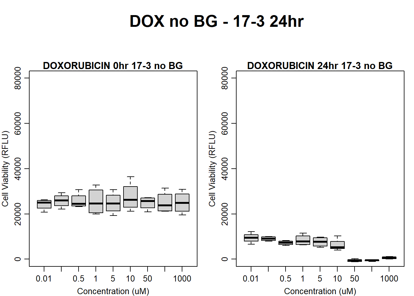
#dox 17-3 24HR
par(mar = c(3.0, 3.0, 1.2, 1), mgp = c(2, .7, 0))
layout(matrix(c(1, 2, 1, 3), nrow = 2, ncol = 2), heights = c(0.5, 2, 2, 2))
#layout.show(3)
plot.new()
text(0.5,0.5,"DOX no BG - 17-3 24hr",cex = 2,font = 2)

boxplot(dox24hr17$Ind3_17_In_noBG ~ dox24hr17$Conc,
        ylim = c(0, 80000),
        ylab = "Cell Viability (RFLU)",
        xlab = "Concentration (uM)",
        main = "DOXORUBICIN 0hr 17-3 no BG"
)

boxplot(dox24hr17$Ind3_17_Fin_noBG ~ dox24hr17$Conc,
        ylim = c(0,80000),
        ylab = "Cell Viability (RFLU)",
        xlab = "Concentration (uM)",
        main = "DOXORUBICIN 24hr 17-3 no BG"
)
| Version | Author | Date |
|---|---|---|
| 0f7b54c | emmapfort | 2025-12-01 |
#####DMSO samples#####
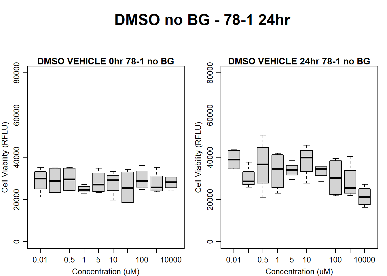
#DMSO 78-1 24HR
par(mar = c(3.0, 3.0, 1.2, 1), mgp = c(2, .7, 0))
layout(matrix(c(1, 2, 1, 3), nrow = 2, ncol = 2), heights = c(0.5, 2, 2, 2))
#layout.show(3)
plot.new()
text(0.5,0.5,"DMSO no BG - 78-1 24hr",cex = 2,font = 2)
boxplot(dmso24hr78$Ind2_78_In_noBG ~ dmso24hr78$Conc,
ylim = c(0, 80000),
ylab = "Cell Viability (RFLU)",
xlab = "Concentration (uM)",
main = "DMSO VEHICLE 0hr 78-1 no BG"
)
boxplot(dmso24hr78$Ind2_78_Fin_noBG ~ dmso24hr78$Conc,
ylim = c(0,80000),
ylab = "Cell Viability (RFLU)",
xlab = "Concentration (uM)",
main = "DMSO VEHICLE 24hr 78-1 no BG"
)
| Version | Author | Date |
|---|---|---|
| 0f7b54c | emmapfort | 2025-12-01 |
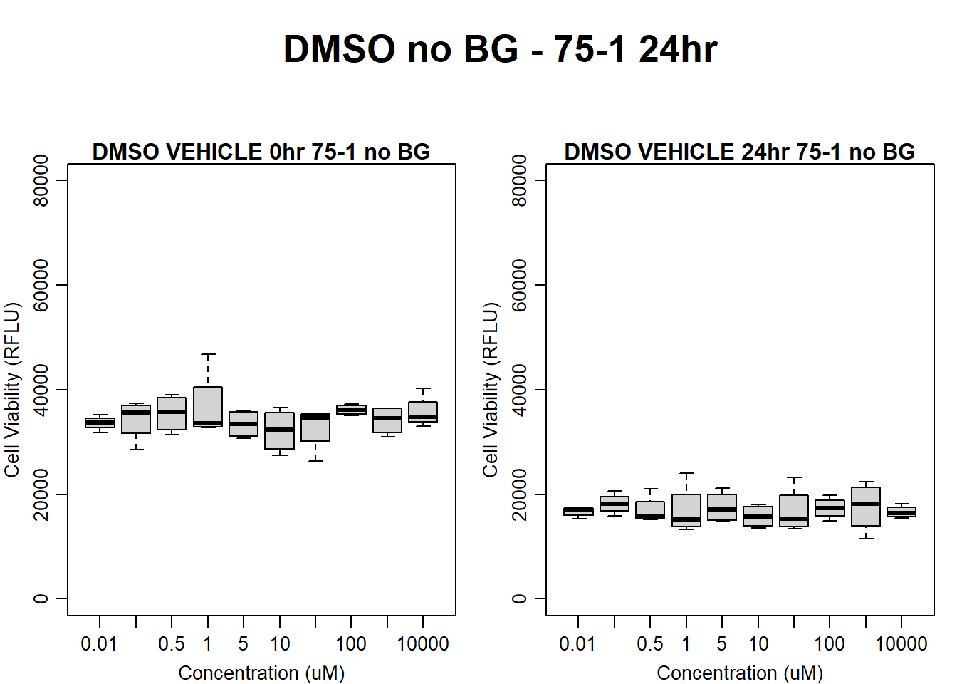
#DMSO 75-1 no BG 24HR
par(mar = c(3.0, 3.0, 1.2, 1), mgp = c(2, .7, 0))
layout(matrix(c(1, 2, 1, 3), nrow = 2, ncol = 2), heights = c(0.5, 2, 2, 2))
#layout.show(3)
plot.new()
text(0.5,0.5,"DMSO no BG - 75-1 24hr",cex = 2,font = 2)

boxplot(dmso24hr75$Ind1_75_In_noBG ~ dmso24hr75$Conc,
        ylim = c(0, 80000),
        ylab = "Cell Viability (RFLU)",
        xlab = "Concentration (uM)",
        main = "DMSO VEHICLE 0hr 75-1 no BG"
)

boxplot(dmso24hr75$Ind1_75_Fin_noBG ~ dmso24hr75$Conc,
        ylim = c(0,80000),
        ylab = "Cell Viability (RFLU)",
        xlab = "Concentration (uM)",
        main = "DMSO VEHICLE 24hr 75-1 no BG"
)
| Version | Author | Date |
|---|---|---|
| 0f7b54c | emmapfort | 2025-12-01 |
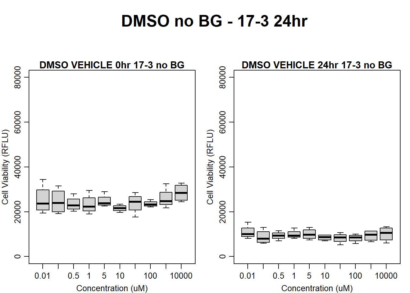
#DMSO 17-3 no BG 24HR
par(mar = c(3.0, 3.0, 1.2, 1), mgp = c(2, .7, 0))
layout(matrix(c(1, 2, 1, 3), nrow = 2, ncol = 2), heights = c(0.5, 2, 2, 2))
#layout.show(3)
plot.new()
text(0.5,0.5,"DMSO no BG - 17-3 24hr",cex = 2,font = 2)

boxplot(dmso24hr17$Ind3_17_In_noBG ~ dmso24hr17$Conc,
        ylim = c(0, 80000),
        ylab = "Cell Viability (RFLU)",
        xlab = "Concentration (uM)",
        main = "DMSO VEHICLE 0hr 17-3 no BG"
)

boxplot(dmso24hr17$Ind3_17_Fin_noBG ~ dmso24hr17$Conc,
        ylim = c(0,80000),
        ylab = "Cell Viability (RFLU)",
        xlab = "Concentration (uM)",
        main = "DMSO VEHICLE 24hr 17-3 no BG"
)
| Version | Author | Date |
|---|---|---|
| 0f7b54c | emmapfort | 2025-12-01 |
Now let’s plot the next step: subtracting the empty wells
Subtract Empty Wells
#####DOX Samples#####
#dox 78-1 Empty Wells 24HR
par(mar = c(3.0, 3.0, 1.2, 1), mgp = c(2, .7, 0))
layout(matrix(c(1, 2, 1, 3), nrow = 2, ncol = 2), heights = c(0.5, 2, 2, 2))
#layout.show(3)
plot.new()
text(0.5,0.5,"DOX no BG Empty - 78-1 24hr",cex = 2,font = 2)

boxplot(dox24hr78$Ind2_78_In_noBG_Low ~ dox24hr78$Conc,
        ylim = c(0, 1.5),
        ylab = "Cell Viability (%)",
        xlab = "Concentration (uM)",
        main = "DOXORUBICIN 0hr 78-1 no BG Empty"
)

boxplot(dox24hr78$Ind2_78_Fin_noBG_Low ~ dox24hr78$Conc,
        ylim = c(0, 1.5),
        ylab = "Cell Viability (%)",
        xlab = "Concentration (uM)",
        main = "DOXORUBICIN 24hr 78-1 no BG"
)![]()
| Version | Author | Date |
|---|---|---|
| 0f7b54c | emmapfort | 2025-12-01 |
#dox 75-1 24HR
par(mar = c(3.0, 3.0, 1.2, 1), mgp = c(2, .7, 0))
layout(matrix(c(1, 2, 1, 3), nrow = 2, ncol = 2), heights = c(0.5, 2, 2, 2))
#layout.show(3)
plot.new()
text(0.5,0.5,"DOX no BG Empty - 75-1 24hr",cex = 2,font = 2)

boxplot(dox24hr75$Ind1_75_In_noBG_Low ~ dox24hr75$Conc,
        ylim = c(0, 1.5),
        ylab = "Cell Viability (%)",
        xlab = "Concentration (uM)",
        main = "DOXORUBICIN 0hr 75-1 no BG Empty"
)

boxplot(dox24hr75$Ind1_75_Fin_noBG_Low ~ dox24hr75$Conc,
        ylim = c(0, 1.5),
        ylab = "Cell Viability (%)",
        xlab = "Concentration (uM)",
        main = "DOXORUBICIN 24hr 75-1 no BG Empty"
)![]()
| Version | Author | Date |
|---|---|---|
| 0f7b54c | emmapfort | 2025-12-01 |
#dox 17-3 24HR
par(mar = c(3.0, 3.0, 1.2, 1), mgp = c(2, .7, 0))
layout(matrix(c(1, 2, 1, 3), nrow = 2, ncol = 2), heights = c(0.5, 2, 2, 2))
#layout.show(3)
plot.new()
text(0.5,0.5,"DOX no BG Empty - 17-3 24hr",cex = 2,font = 2)

boxplot(dox24hr17$Ind3_17_In_noBG_Low ~ dox24hr17$Conc,
        ylim = c(0, 1.5),
        ylab = "Cell Viability (%)",
        xlab = "Concentration (uM)",
        main = "DOXORUBICIN 0hr 17-3 no BG Empty"
)

boxplot(dox24hr17$Ind3_17_Fin_noBG_Low ~ dox24hr17$Conc,
        ylim = c(0, 1.5),
        ylab = "Cell Viability (%)",
        xlab = "Concentration (uM)",
        main = "DOXORUBICIN 24hr 17-3 no BG Empty"
)![]()
| Version | Author | Date |
|---|---|---|
| 0f7b54c | emmapfort | 2025-12-01 |
#####DMSO samples#####
#DMSO 78-1 24HR
par(mar = c(3.0, 3.0, 1.2, 1), mgp = c(2, .7, 0))
layout(matrix(c(1, 2, 1, 3), nrow = 2, ncol = 2), heights = c(0.5, 2, 2, 2))
#layout.show(3)
plot.new()
text(0.5,0.5,"DMSO no BG Empty - 78-1 24hr",cex = 2,font = 2)

boxplot(dmso24hr78$Ind2_78_In_noBG_Low ~ dmso24hr78$Conc,
        ylim = c(0, 1.5),
        ylab = "Cell Viability (%)",
        xlab = "Concentration (uM)",
        main = "DMSO VEHICLE 0hr 78-1 no BG Empty"
)

boxplot(dmso24hr78$Ind2_78_Fin_noBG_Low ~ dmso24hr78$Conc,
        ylim = c(0, 1.5),
        ylab = "Cell Viability (%)",
        xlab = "Concentration (uM)",
        main = "DMSO VEHICLE 24hr 78-1 no BG Empty"
)![]()
| Version | Author | Date |
|---|---|---|
| 0f7b54c | emmapfort | 2025-12-01 |
#DMSO 75-1 no BG Empty 24HR
par(mar = c(3.0, 3.0, 1.2, 1), mgp = c(2, .7, 0))
layout(matrix(c(1, 2, 1, 3), nrow = 2, ncol = 2), heights = c(0.5, 2, 2, 2))
#layout.show(3)
plot.new()
text(0.5,0.5,"DMSO no BG Empty - 75-1 24hr",cex = 2,font = 2)

boxplot(dmso24hr75$Ind1_75_In_noBG_Low ~ dmso24hr75$Conc,
        ylim = c(0, 1.5),
        ylab = "Cell Viability (%)",
        xlab = "Concentration (uM)",
        main = "DMSO VEHICLE 0hr 75-1 no BG Empty"
)

boxplot(dmso24hr75$Ind1_75_Fin_noBG_Low ~ dmso24hr75$Conc,
        ylim = c(0, 1.5),
        ylab = "Cell Viability (%)",
        xlab = "Concentration (uM)",
        main = "DMSO VEHICLE 24hr 75-1 no BG Empty"
)![]()
| Version | Author | Date |
|---|---|---|
| 0f7b54c | emmapfort | 2025-12-01 |
#DMSO 17-3 no BG Empty 24HR
par(mar = c(3.0, 3.0, 1.2, 1), mgp = c(2, .7, 0))
layout(matrix(c(1, 2, 1, 3), nrow = 2, ncol = 2), heights = c(0.5, 2, 2, 2))
#layout.show(3)
plot.new()
text(0.5,0.5,"DMSO no BG Empty - 17-3 24hr",cex = 2,font = 2)

boxplot(dmso24hr17$Ind3_17_In_noBG_Low ~ dmso24hr17$Conc,
        ylim = c(0, 1.5),
        ylab = "Cell Viability (%)",
        xlab = "Concentration (uM)",
        main = "DMSO VEHICLE 0hr 17-3 no BG Empty"
)

boxplot(dmso24hr17$Ind3_17_Fin_noBG_Low ~ dmso24hr17$Conc,
        ylim = c(0, 1.5),
        ylab = "Cell Viability (%)",
        xlab = "Concentration (uM)",
        main = "DMSO VEHICLE 24hr 17-3 no BG Empty"
)![]()
| Version | Author | Date |
|---|---|---|
| 0f7b54c | emmapfort | 2025-12-01 |
Now let’s plot the third step: dividing the matched vehicle values
Divide by Matched Vehicle
#####DOX Samples#####
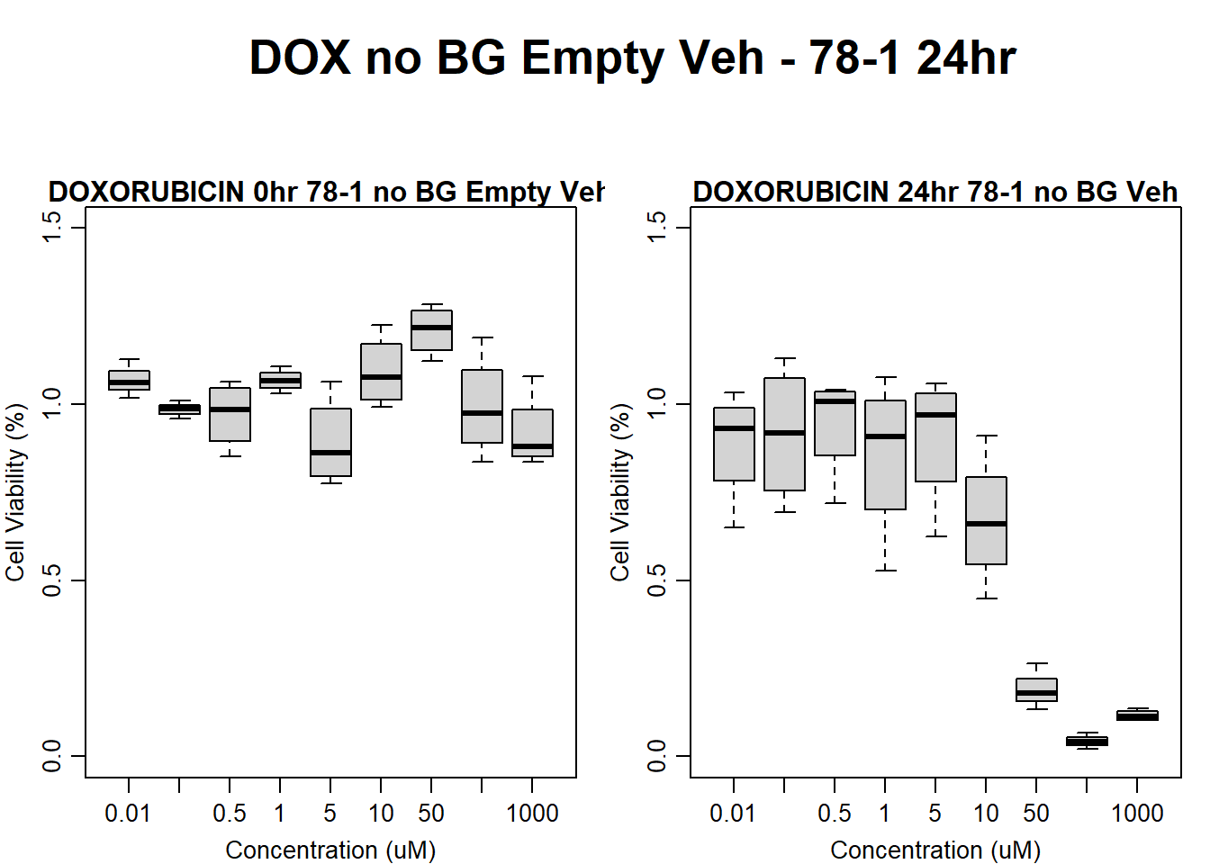
#dox 78-1 Veh 24HR
par(mar = c(3.0, 3.0, 1.2, 1), mgp = c(2, .7, 0))
layout(matrix(c(1, 2, 1, 3), nrow = 2, ncol = 2), heights = c(0.5, 2, 2, 2))
#layout.show(3)
plot.new()
text(0.5,0.5,"DOX no BG Empty Veh - 78-1 24hr",cex = 2,font = 2)
boxplot(dox24hr78$Ind2_78_In_noBG_Low_Veh ~ dox24hr78$Conc,
ylim = c(0, 1.5),
ylab = "Cell Viability (%)",
xlab = "Concentration (uM)",
main = "DOXORUBICIN 0hr 78-1 no BG Empty Veh"
)
boxplot(dox24hr78$Ind2_78_Fin_noBG_Low_Veh ~ dox24hr78$Conc,
ylim = c(0, 1.5),
ylab = "Cell Viability (%)",
xlab = "Concentration (uM)",
main = "DOXORUBICIN 24hr 78-1 no BG Veh"
)
| Version | Author | Date |
|---|---|---|
| 0f7b54c | emmapfort | 2025-12-01 |
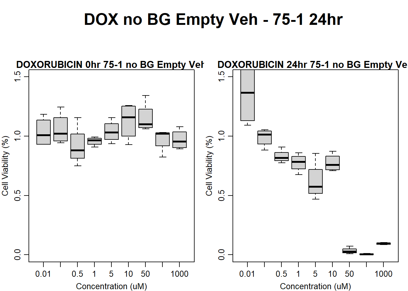
#dox 75-1 24HR
par(mar = c(3.0, 3.0, 1.2, 1), mgp = c(2, .7, 0))
layout(matrix(c(1, 2, 1, 3), nrow = 2, ncol = 2), heights = c(0.5, 2, 2, 2))
#layout.show(3)
plot.new()
text(0.5,0.5,"DOX no BG Empty Veh - 75-1 24hr",cex = 2,font = 2)

boxplot(dox24hr75$Ind1_75_In_noBG_Low_Veh ~ dox24hr75$Conc,
        ylim = c(0, 1.5),
        ylab = "Cell Viability (%)",
        xlab = "Concentration (uM)",
        main = "DOXORUBICIN 0hr 75-1 no BG Empty Veh"
)

boxplot(dox24hr75$Ind1_75_Fin_noBG_Low_Veh ~ dox24hr75$Conc,
        ylim = c(0, 1.5),
        ylab = "Cell Viability (%)",
        xlab = "Concentration (uM)",
        main = "DOXORUBICIN 24hr 75-1 no BG Empty Veh"
)
| Version | Author | Date |
|---|---|---|
| 0f7b54c | emmapfort | 2025-12-01 |
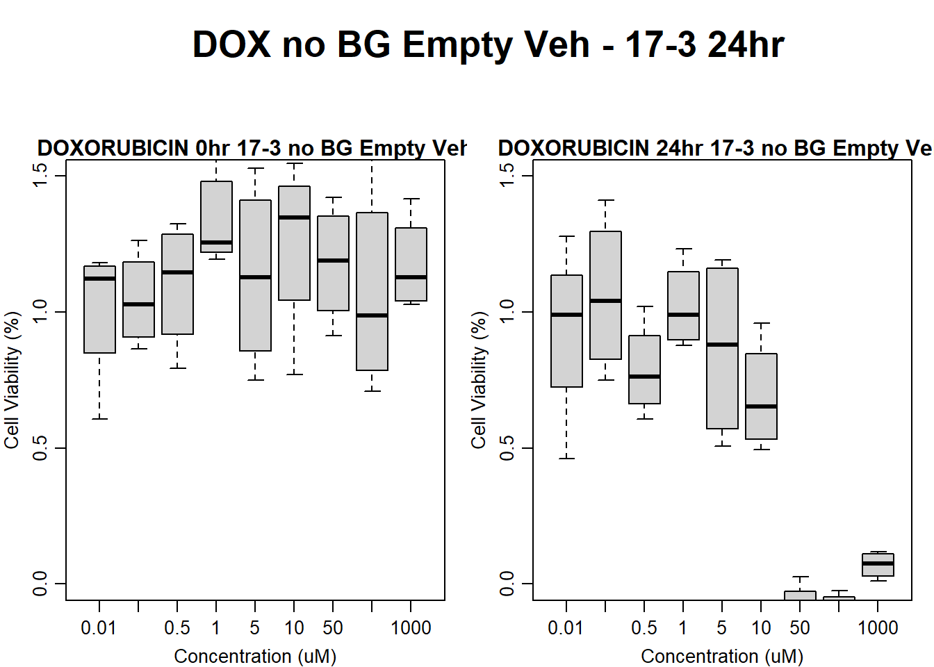
#dox 17-3 24HR
par(mar = c(3.0, 3.0, 1.2, 1), mgp = c(2, .7, 0))
layout(matrix(c(1, 2, 1, 3), nrow = 2, ncol = 2), heights = c(0.5, 2, 2, 2))
#layout.show(3)
plot.new()
text(0.5,0.5,"DOX no BG Empty Veh - 17-3 24hr",cex = 2,font = 2)

boxplot(dox24hr17$Ind3_17_In_noBG_Low_Veh ~ dox24hr17$Conc,
        ylim = c(0, 1.5),
        ylab = "Cell Viability (%)",
        xlab = "Concentration (uM)",
        main = "DOXORUBICIN 0hr 17-3 no BG Empty Veh"
)

boxplot(dox24hr17$Ind3_17_Fin_noBG_Low_Veh ~ dox24hr17$Conc,
        ylim = c(0, 1.5),
        ylab = "Cell Viability (%)",
        xlab = "Concentration (uM)",
        main = "DOXORUBICIN 24hr 17-3 no BG Empty Veh"
)
| Version | Author | Date |
|---|---|---|
| 0f7b54c | emmapfort | 2025-12-01 |
#####DMSO samples#####
#DMSO 78-1 24HR
par(mar = c(3.0, 3.0, 1.2, 1), mgp = c(2, .7, 0))
layout(matrix(c(1, 2, 1, 3), nrow = 2, ncol = 2), heights = c(0.5, 2, 2, 2))
#layout.show(3)
plot.new()
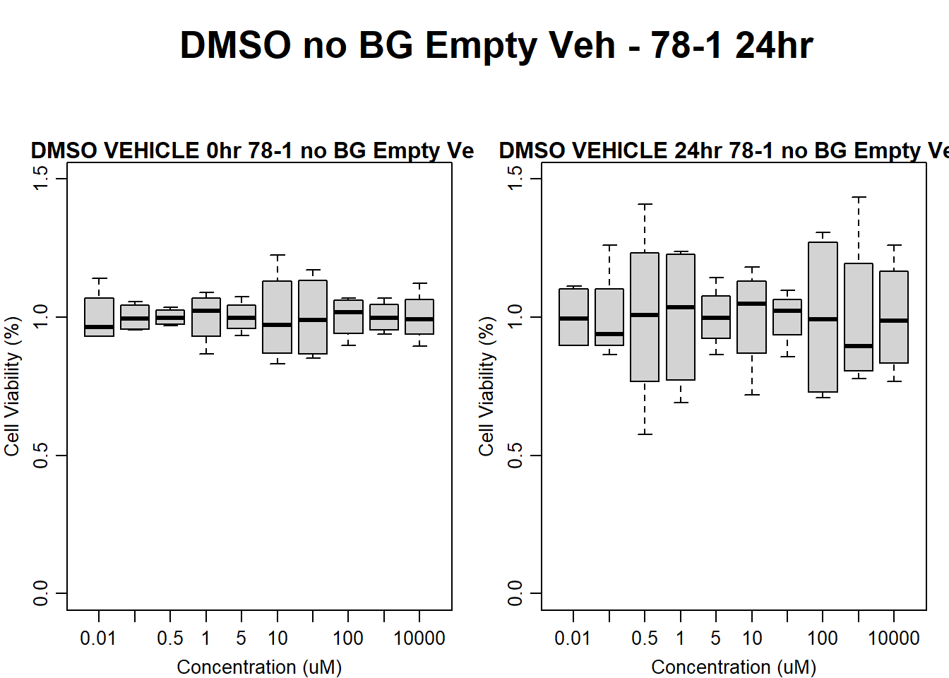
text(0.5,0.5,"DMSO no BG Empty Veh - 78-1 24hr",cex = 2,font = 2)
boxplot(dmso24hr78$Ind2_78_In_noBG_Low_Veh ~ dmso24hr78$Conc,
ylim = c(0, 1.5),
ylab = "Cell Viability (%)",
xlab = "Concentration (uM)",
main = "DMSO VEHICLE 0hr 78-1 no BG Empty Veh"
)
boxplot(dmso24hr78$Ind2_78_Fin_noBG_Low_Veh ~ dmso24hr78$Conc,
ylim = c(0, 1.5),
ylab = "Cell Viability (%)",
xlab = "Concentration (uM)",
main = "DMSO VEHICLE 24hr 78-1 no BG Empty Veh"
)
| Version | Author | Date |
|---|---|---|
| 0f7b54c | emmapfort | 2025-12-01 |
#DMSO 75-1 no BG Empty 24HR
par(mar = c(3.0, 3.0, 1.2, 1), mgp = c(2, .7, 0))
layout(matrix(c(1, 2, 1, 3), nrow = 2, ncol = 2), heights = c(0.5, 2, 2, 2))
#layout.show(3)
plot.new()
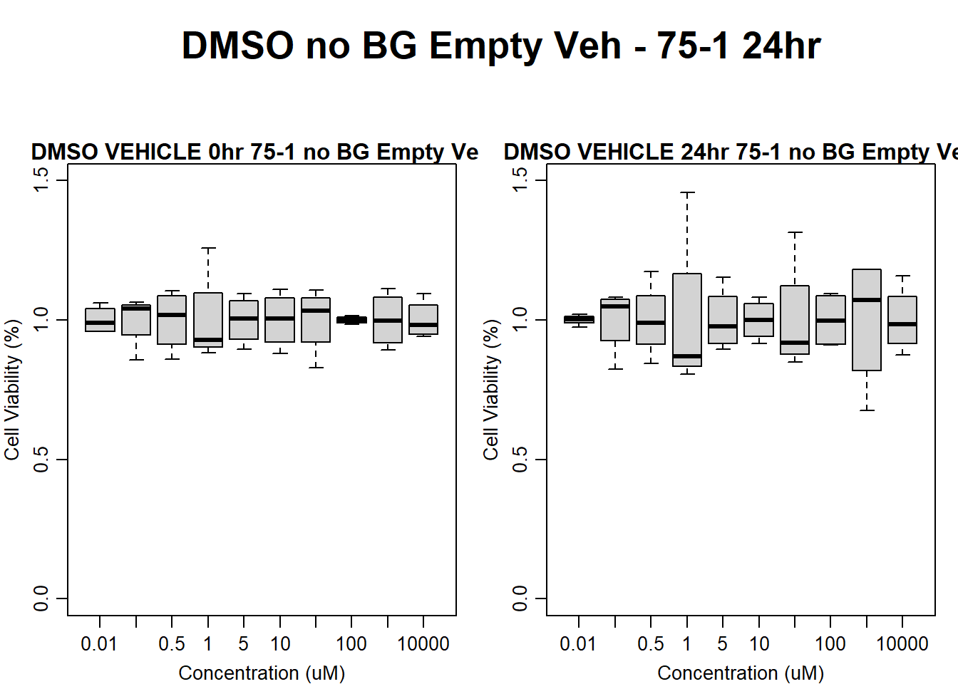
text(0.5,0.5,"DMSO no BG Empty Veh - 75-1 24hr",cex = 2,font = 2)
boxplot(dmso24hr75$Ind1_75_In_noBG_Low_Veh ~ dmso24hr75$Conc,
ylim = c(0, 1.5),
ylab = "Cell Viability (%)",
xlab = "Concentration (uM)",
main = "DMSO VEHICLE 0hr 75-1 no BG Empty Veh"
)
boxplot(dmso24hr75$Ind1_75_Fin_noBG_Low_Veh ~ dmso24hr75$Conc,
ylim = c(0, 1.5),
ylab = "Cell Viability (%)",
xlab = "Concentration (uM)",
main = "DMSO VEHICLE 24hr 75-1 no BG Empty Veh"
)
| Version | Author | Date |
|---|---|---|
| 0f7b54c | emmapfort | 2025-12-01 |
#DMSO 17-3 no BG Empty 24HR
par(mar = c(3.0, 3.0, 1.2, 1), mgp = c(2, .7, 0))
layout(matrix(c(1, 2, 1, 3), nrow = 2, ncol = 2), heights = c(0.5, 2, 2, 2))
#layout.show(3)
plot.new()
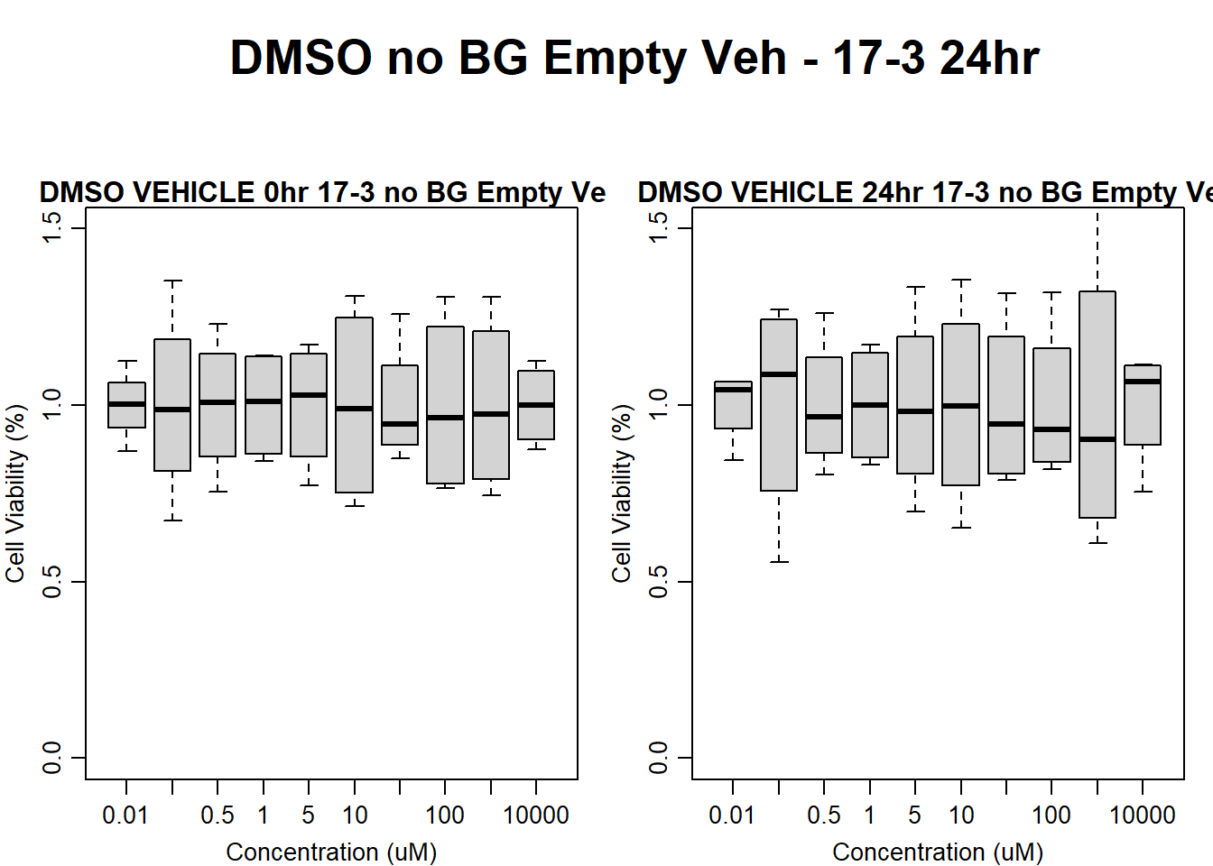
text(0.5,0.5,"DMSO no BG Empty Veh - 17-3 24hr",cex = 2,font = 2)
boxplot(dmso24hr17$Ind3_17_In_noBG_Low_Veh ~ dmso24hr17$Conc,
ylim = c(0, 1.5),
ylab = "Cell Viability (%)",
xlab = "Concentration (uM)",
main = "DMSO VEHICLE 0hr 17-3 no BG Empty Veh"
)
boxplot(dmso24hr17$Ind3_17_Fin_noBG_Low_Veh ~ dmso24hr17$Conc,
ylim = c(0, 1.5),
ylab = "Cell Viability (%)",
xlab = "Concentration (uM)",
main = "DMSO VEHICLE 24hr 17-3 no BG Empty Veh"
)
| Version | Author | Date |
|---|---|---|
| 0f7b54c | emmapfort | 2025-12-01 |
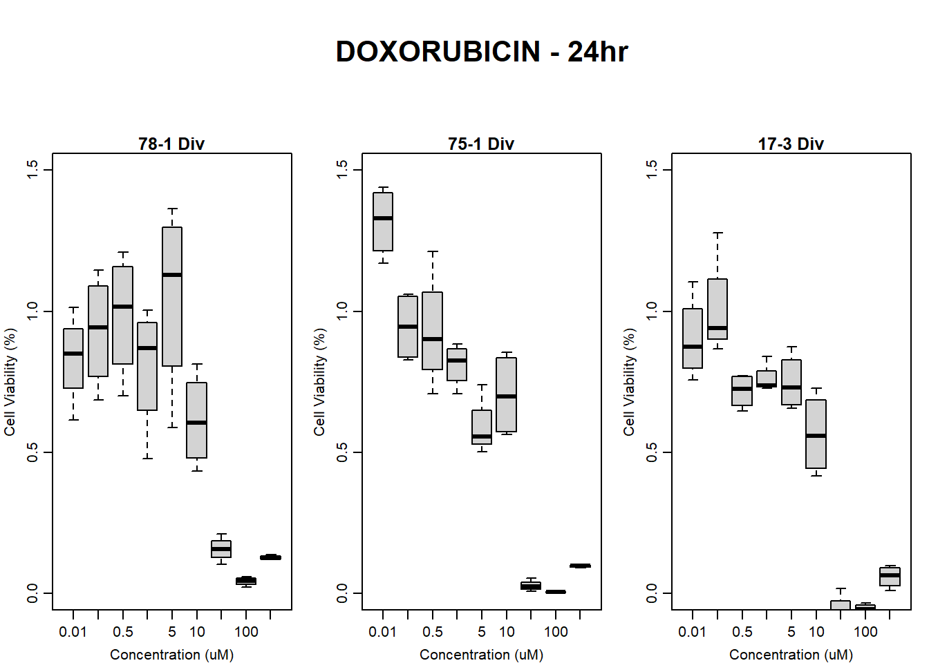
Now for the final step, dividing the final timepoint by the initial baseline reading at 0hr
Divide Final Timepoint by Baseline
#####DOX Samples#####
#dox All 24HR
par(mar = c(3.0, 3.0, 1.2, 1), mgp = c(2, .7, 0))
layout(matrix(c(1, 2, 1, 3, 1, 4), nrow = 2, ncol = 3), heights = c(0.5, 2, 2, 2))
#layout.show(3)
plot.new()
text(0.5,0.5,"DOXORUBICIN - 24hr",cex = 2,font = 2)

boxplot(dox24hr78$Ind2_78_Div ~ dox24hr78$Conc,
        ylim = c(0, 1.5),
        ylab = "Cell Viability (%)",
        xlab = "Concentration (uM)",
        main = "78-1 Div"
)

boxplot(dox24hr75$Ind1_75_Div ~ dox24hr75$Conc,
        ylim = c(0, 1.5),
        ylab = "Cell Viability (%)",
        xlab = "Concentration (uM)",
        main = "75-1 Div"
)

boxplot(dox24hr17$Ind3_17_Div ~ dox24hr17$Conc,
        ylim = c(0, 1.5),
        ylab = "Cell Viability (%)",
        xlab = "Concentration (uM)",
        main = "17-3 Div"
)
| Version | Author | Date |
|---|---|---|
| 0f7b54c | emmapfort | 2025-12-01 |
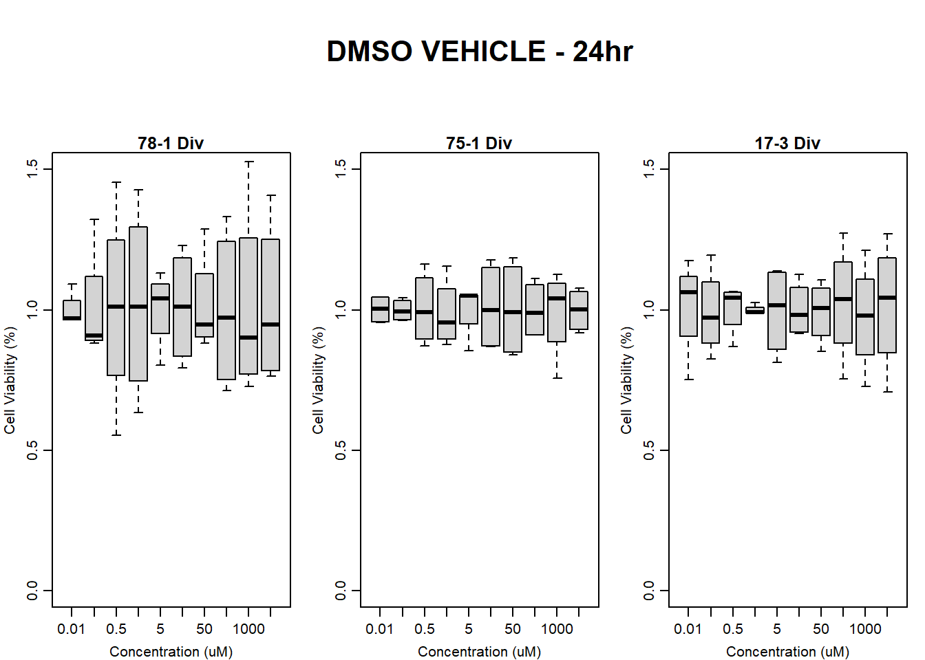
#####DMSO samples#####
#DMSO All 24HR
par(mar = c(3.0, 3.0, 1.2, 1), mgp = c(2, .7, 0))
layout(matrix(c(1, 2, 1, 3, 1, 4), nrow = 2, ncol = 3), heights = c(0.5, 2, 2, 2))
#layout.show(3)
plot.new()
text(0.5,0.5,"DMSO VEHICLE - 24hr",cex = 2,font = 2)

boxplot(dmso24hr78$Ind2_78_Div ~ dmso24hr78$Conc,
        ylim = c(0, 1.5),
        ylab = "Cell Viability (%)",
        xlab = "Concentration (uM)",
        main = "78-1 Div"
)

boxplot(dmso24hr75$Ind1_75_Div ~ dmso24hr75$Conc,
        ylim = c(0, 1.5),
        ylab = "Cell Viability (%)",
        xlab = "Concentration (uM)",
        main = "75-1 Div"
)

boxplot(dmso24hr17$Ind3_17_Div ~ dmso24hr17$Conc,
        ylim = c(0, 1.5),
        ylab = "Cell Viability (%)",
        xlab = "Concentration (uM)",
        main = "17-3 Div"
)
| Version | Author | Date |
|---|---|---|
| 0f7b54c | emmapfort | 2025-12-01 |
Fit Models for DRC
#these sheets are not numbered properly by individual because they're in order of experiments
dox24tox_75 <- dox24hr75 %>% mutate(response = Ind1_75_Div*100)
summary(dox24tox_75$response)
Min. 1st Qu. Median Mean 3rd Qu. Max.
0.2582 9.4402 70.8116 60.2731 88.1141 143.8750 dox24tox_78 <- dox24hr78 %>% mutate(response = Ind2_78_Div*100)
summary(dox24tox_78$response) Min. 1st Qu. Median Mean 3rd Qu. Max.
2.304 14.760 68.363 61.596 94.656 136.295 dox24tox_17 <- dox24hr17 %>% mutate(response = Ind3_17_Div*100)
summary(dox24tox_17$response) Min. 1st Qu. Median Mean 3rd Qu. Max.
-12.545 3.773 68.230 51.372 79.390 127.911 #Fit Models
doxtox24_78_model <- drm(response ~ Conc, data = dox24tox_78, fct = LL.4(fixed = c(NA, 0, 100, NA)))
doxtox24_75_model <- drm(response ~ Conc, data = dox24tox_75, fct = LL.4(fixed = c(NA, 0, 100, NA)))
doxtox24_17_model <- drm(response ~ Conc, data = dox24tox_17, fct = LL.4(fixed = c(NA, 0, 100, NA)))
#Add in labels
conc_labels <- c(0.01, 0.1, 0.5, 1, 10, 50, 100, 1000)
pct_labels <- c(0, 10, 20, 30, 40, 50, 60, 70, 80, 90, 100)
#extract LD50
ed75 <- ED(doxtox24_78_model, 50, interval = "delta")[1]
Estimated effective doses

       Estimate Std. Error   Lower   Upper
e:1:50  16.1179     4.4686  7.0366 25.1993
ed78 <- ED(doxtox24_75_model, 50, interval = "delta")[1]
Estimated effective doses

       Estimate Std. Error   Lower   Upper
e:1:50  10.0892     2.3992  5.2134 14.9649
ed17 <- ED(doxtox24_17_model, 50, interval = "delta")[1]
Estimated effective doses

       Estimate Std. Error   Lower   Upper
e:1:50   9.7850     1.7753  6.1771 13.3928
#find the median ld50 for plotting
median_ld50 <- median(c(ed78, ed75, ed17))Plot DRC
# Define output folder and base filename
# output_folder
# base_name <- "viability_curve_scaled"

# Full file paths
# png_path <- file.path(output_folder, paste0(base_name, ".png"))
# svg_path <- file.path(output_folder, paste0(base_name, ".svg"))
# pdf_path <- file.path(output_folder, paste0(base_name, ".pdf"))

# New scaled dimensions (2x)
# plot_height <- 7.3212
# plot_width<- 3.8604
# plot_width <- 5.7906

#export as a png
# png(filename = png_path,
#     width = plot_width, height = plot_height,
#     units = "in", res = 300)

#plot code as above in finalized version
plot(doxtox24_78_model, type = "none", broken = TRUE,
     ylim = c(0,100), col = "#9ACCDE", lwd = 3,
     ylab = "Percent Viability (%)", xlab = "Concentration (uM)",
     main = "24hr Treatment", log = "x", axes = FALSE)
plot(doxtox24_75_model, add = TRUE, col = "#499FBD", lwd = 3, type = "none")
plot(doxtox24_17_model, add = TRUE, col = "#254F5E", lwd = 3, type = "none")

axis(1, at = conc_labels, labels = conc_labels, las = 2, cex.axis = 1)
axis(2, at = pct_labels, labels = pct_labels, las = 2, cex.axis = 0.9)

abline(v = 0.5, col = "grey50", lty = 2, lwd = 2)
abline(v = median_ld50, col = "red", lty = 3, lwd = 2)
text(x = median_ld50, y = 99,
     labels = paste0("Median LD50"),
     col = "red", pos = 4, cex = 1, font = 2)

legend("bottomleft",
       legend = c(
         paste0("Ind3 (LD50 = ", round(ed78, 2), " µM)"),
         paste0("Ind4 (LD50 = ", round(ed75, 2), " µM)"),
         paste0("Ind5 (LD50 = ", round(ed17, 2), " µM)")
       ),
       col = c("#9ACCDE", "#499FBD", "#254F5E"),
       lwd = 3, lty = c(1,1,1), cex = 1,
       title = "Individuals")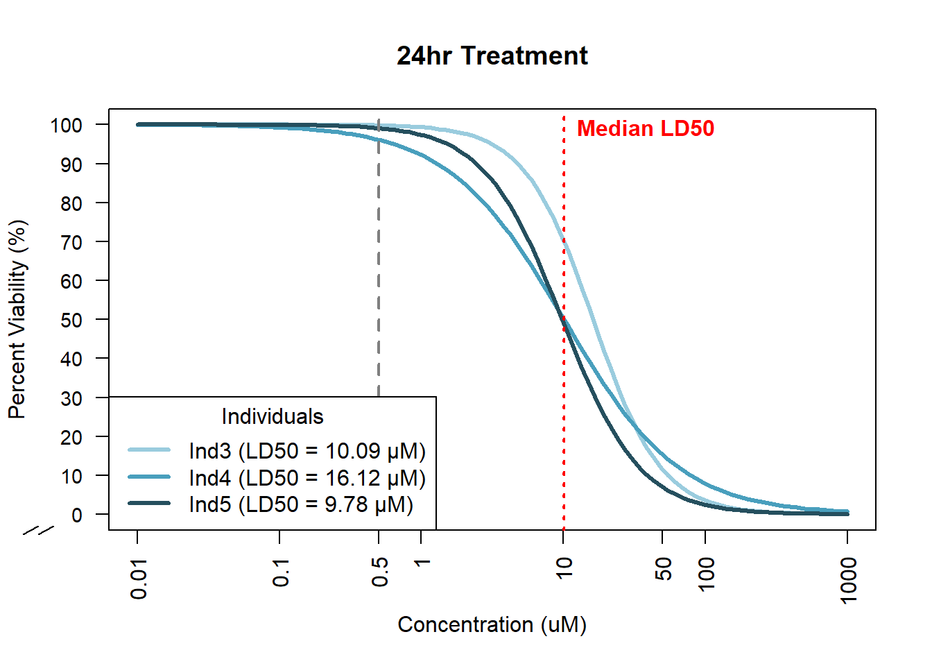
| Version | Author | Date |
|---|---|---|
| 0f7b54c | emmapfort | 2025-12-01 |
# dev.off()

#export as svg
# svg(filename = svg_path,
#     width = plot_width, height = plot_height)

#repeat plotting code with same adjustments
# plot(doxtox24_78_model, type = "none", broken = TRUE,
#      ylim = c(0,100), col = "#9ACCDE", lwd = 3,
#      ylab = "Percent Viability (%)", xlab = "Concentration (uM)",
#      main = "24hr Treatment", log = "x", axes = FALSE)
# plot(doxtox24_75_model, add = TRUE, col = "#499FBD", lwd = 3, type = "none")
# plot(doxtox24_17_model, add = TRUE, col = "#254F5E", lwd = 3, type = "none")
# axis(1, at = conc_labels, labels = conc_labels, las = 2, cex.axis = 1)
# axis(2, at = pct_labels, labels = pct_labels, las = 2, cex.axis = 0.9)
# abline(v = 0.5, col = "grey50", lty = 2, lwd = 2)
# abline(v = median_ld50, col = "red", lty = 3, lwd = 2)
# text(x = median_ld50, y = 99,
#      labels = paste0("Median LD50"),
#      col = "red", pos = 4, cex = 1, font = 2)
# legend("bottomleft",
#        legend = c(
#          paste0("Ind3 (LD50 = ", round(ed78, 2), " µM)"),
#          paste0("Ind4 (LD50 = ", round(ed75, 2), " µM)"),
#          paste0("Ind5 (LD50 = ", round(ed17, 2), " µM)")
#        ),
#        col = c("#9ACCDE", "#499FBD", "#254F5E"),
#        lwd = 3, lty = c(1,1,1), cex = 1,
#        title = "Individuals")

# dev.off()

#export as pdf
# pdf(file = pdf_path,
#     width = plot_width, height = plot_height)

#repeat plotting code again to print
# plot(doxtox24_78_model, type = "none", broken = TRUE,
#      ylim = c(0,100), col = "#9ACCDE", lwd = 3,
#      ylab = "Percent Viability (%)", xlab = "Concentration (uM)",
#      main = "24hr Treatment", log = "x", axes = FALSE)
# plot(doxtox24_75_model, add = TRUE, col = "#499FBD", lwd = 3, type = "none")
# plot(doxtox24_17_model, add = TRUE, col = "#254F5E", lwd = 3, type = "none")
# axis(1, at = conc_labels, labels = conc_labels, las = 2, cex.axis = 1)
# axis(2, at = pct_labels, labels = pct_labels, las = 2, cex.axis = 0.9)
# abline(v = 0.5, col = "grey50", lty = 2, lwd = 2)
# abline(v = median_ld50, col = "red", lty = 3, lwd = 2)
# text(x = median_ld50, y = 99,
#      labels = paste0("Median LD50"),
#      col = "red", pos = 4, cex = 1, font = 2)
# legend("bottomleft",
#        legend = c(
#          paste0("Ind3 (LD50 = ", round(ed78, 2), " µM)"),
#          paste0("Ind4 (LD50 = ", round(ed75, 2), " µM)"),
#          paste0("Ind5 (LD50 = ", round(ed17, 2), " µM)")
#        ),
#        col = c("#9ACCDE", "#499FBD", "#254F5E"),
#        lwd = 3, lty = c(1,1,1), cex = 1,
#        title = "Individuals")

# dev.off()

#saved code for saving the plots for posterity!
Figure 1D - DNA Damage Quantification
yH2AX Quantification (Immunofluorescence Staining).
Fiji/ImageJ Macros
Macros used in ImageJ/Fiji to identify nuclear ROIs from yH2AX IF staining.
#these are the macros that I made for ImageJ/Fiji and are included for reference only
#they will not run in R

#DAPI ROI generator macro to split DAPI channel and map nuclei
# // === STEP 1: Define folders ===
# folder = "D:\\DXR Project\\IF yH2AX\\if yh2ax dxr 84-1\\rgb quant\\";
# saveRoiFolder = "D:\\DXR Project\\IF yH2AX\\if yh2ax dxr 84-1\\outline new\\";
# saveRedFolder = "D:\\DXR Project\\IF yH2AX\\if yh2ax dxr 84-1\\TxRed new\\";
#
# list = getFileList(folder);
#
# for (i = 0; i < list.length; i++) {
#     if (endsWith(list[i], ".tif")) {
#         print("----------------------------------------------------");
#         print("Processing file: " + list[i]);
#
#         // Open composite image
#         open(folder + list[i]);
#         originalTitle = getTitle();
#         baseName = replace(list[i], ".tif", "");
#
#         // === STEP 2: Duplicate and close original ===
#         newTitle = baseName + "_proc";
#         run("Duplicate...", "title=" + newTitle);
#         dupTitle = getTitle();
#         print("Created duplicate: " + dupTitle);
#
#         selectImage(originalTitle);
#         close();
#         print("Closed original composite: " + originalTitle);
#
#         // === STEP 3: Split channels of duplicate ===
#         selectImage(dupTitle);
#         run("Split Channels");
#         print("Split channels from: " + dupTitle);
#
#         // === STEP 4: Save the red channel ===
#         redTitle = newTitle + " (red)";
#         if (isOpen(redTitle)) {
#             selectWindow(redTitle);
#             saveAs("Tiff", saveRedFolder + baseName + "_TxRed.tif");
#             print("Saved and closed red channel: " + redTitle);
#             close();
#         } else {
#             print("WARNING: Red channel not found for " + baseName);
#         }
#
#         // === STEP 5: Close green channel ===
#         greenTitle = newTitle + " (green)";
#         if (isOpen(greenTitle)) {
#             selectWindow(greenTitle);
#             close();
#             print("Closed green channel: " + greenTitle);
#         } else {
#             print("Green channel not found for " + baseName);
#         }
#
#         // === STEP 6: Process DAPI (blue) channel ===
#         dapiTitle = newTitle + " (blue)";
#         if (isOpen(dapiTitle)) {
#             selectWindow(dapiTitle);
#             rename(baseName + "_DAPI_proc");
#             print("Processing DAPI channel: " + baseName);
#
#             run("8-bit");
#             run("Enhance Contrast...", "saturated=0.3 normalize");  // normalize intensity
#             setAutoThreshold("Otsu");
#             getThreshold(lower, upper);
#             minThreshold = 10;
#             if (lower < minThreshold) lower = minThreshold;
#             setThreshold(lower, 255);
#             //convert and segment nuclei
#             setOption("BlackBackground", false);
#             run("Convert to Mask");
#             run("Watershed");
#
#             run("Analyze Particles...",
#                 "size=21-Infinity circularity=0.30-1.00 show=[Count Masks] display exclude summarize add");
#
#             // === If no ROIs detected, allow manual threshold adjustment ===
#     if (roiManager("count") == 0) {
#         print("⚠️ No ROIs found for: " + baseName + " — manual adjustment required.");
#         selectWindow(baseName + "_DAPI_proc");
#         run("Threshold...");
#         waitForUser("Adjust the threshold manually until nuclei are visible, then click OK.");
#         run("Convert to Mask");
#         run("Watershed");
#
#         // Re-run particle analysis
#         run("Analyze Particles...",
#             "size=21-Infinity circularity=0.30-1.00 show=[Count Masks] display exclude summarize add");
#     }
#
#             // Save ROIs
#             if (roiManager("count") > 0) {
#                 saveName = baseName + "_DAPI.zip";
#                 roiManager("Save", saveRoiFolder + saveName);
#                 print("Saved ROI zip: " + saveName);
#             } else {
#                 print("No ROIs found for: " + baseName);
#             }
#
#             // Cleanup DAPI
#             close();
#             maskTitle = "Count Masks of " + baseName + "_DAPI_proc";
#             if (isOpen(maskTitle)) {
#                 selectWindow(maskTitle);
#                 close();
#                 print("Closed mask window: " + maskTitle);
#             }
#             roiManager("Deselect");
#             roiManager("Reset");
#         } else {
#             print("DAPI channel not found for " + baseName);
#         }
#
#         // === STEP 7: Close duplicate container window if still open ===
#         if (isOpen(dupTitle)) {
#             selectWindow(dupTitle);
#             close();
#             print("Closed duplicate window: " + dupTitle);
#         }
#
#         print("Finished processing file: " + baseName);
#     }
# }

#each time I ran this I just changed the cell line name in the top

#Red Positivity Macro for identifying red pixels within ROIs and accounting for area
# // ==== USER SETTINGS ====
# roiFolder  = "D:\\DXR Project\\IF yH2AX\\if yh2ax dxr 84-1\\outline new\\";
# redImageFolder = "D:\\DXR Project\\IF yH2AX\\if yh2ax dxr 84-1\\TxRed new\\"
# outputFolder = "D:\\DXR Project\\IF yH2AX\\if yh2ax dxr 84-1\\outline new\\analyzed\\";
# imageExt  = ".tif";
# thresholdLow = 20;
# thresholdHigh = 250;
# // ========================
#
# // Clear results table for combined per-ROI data
# run("Clear Results");
#
# // Initialize arrays for summary
# roiAreas = newArray();
# maxInts = newArray();
# meanInts = newArray();
# medianInts = newArray();
# percentReds = newArray();
# nROIsWithRed = 0;
#
# // Get list of ROI ZIP files
# roiFiles = getFileList(roiFolder);
#
# for (f = 0; f < roiFiles.length; f++) {
#     roiFile = roiFiles[f];
#     if (!endsWith(roiFile, "_DAPI.zip")) continue;
#
#     // Build corresponding red image filename
#     base = replace(roiFile, "_DAPI.zip", "");
#     redImageName = base + "_TxRed.tif";
#     redImagePath = redImageFolder + redImageName;
#
#     print("Trying to open red image: " + redImagePath);
#
#     if (!File.exists(redImagePath)) {
#         print("Red image not found for " + roiFile + ", skipping.");
#         continue;
#     }
#
#     roiZipPath = roiFolder + roiFile;
#
#     // Open red image
#     open(redImagePath);
#     redTitle = getTitle();
#     selectWindow(redTitle);
#
#     // Load ROIs
#     roiManager("Reset");
#     roiManager("Open", roiZipPath);
#
#     nROIs = roiManager("Count");
#     for (r = 0; r < nROIs; r++) {
#         roiManager("Select", r);
#         selectWindow(redTitle);
#
#         // Declare measurement variables
#         areaInt = 0;
#         meanInt = 0;
#         minInt = 0;
#         maxInt = 0;
#         stdInt = 0;
#         histogram = newArray(256);
#
#         getStatistics(areaInt, meanInt, minInt, maxInt, stdInt, histogram);
#
#         // Count red-positive pixels
#         redCount = 0;
#         for (p = thresholdLow; p <= thresholdHigh; p++) redCount += histogram[p];
#         if (redCount == 0) continue; // skip ROIs with no red
#
#         percentRed = (redCount / areaInt) * 100;
#         medianIntVal = getMedianFromHistogram(histogram, areaInt);
#
#         // Save per-ROI results
#         row = nResults;
#         setResult("ROI_File", row, roiFile);
#         setResult("ROI_Area", row, areaInt);
#         setResult("Max_Intensity", row, maxInt);
#         setResult("Mean_Intensity", row, meanInt);
#         setResult("Median_Intensity", row, medianIntVal);
#         setResult("Red_Positive_Pixels", row, redCount);
#         setResult("Percent_Red_Positive", row, percentRed);
#         updateResults();
#
#         // Store for summary
#         roiAreas = arrayAdd(roiAreas, areaInt);
#         maxInts = arrayAdd(maxInts, maxInt);
#         meanInts = arrayAdd(meanInts, meanInt);
#         medianInts = arrayAdd(medianInts, medianIntVal);
#         percentReds = arrayAdd(percentReds, percentRed);
#         nROIsWithRed++;
#     }
#
#     close(redTitle);
# }
#
# // Save combined per-ROI CSV
# saveAs("Results", outputFolder + "All_ROIs_Combined.csv");
# print("Combined per-ROI results saved.");
#
# // Build summary table
# run("Clear Results");
#
# totalNuclearArea = sumArray(roiAreas);
#
# setResult("Experiment", 0, roiFolder);
# setResult("N_Nuclei_With_Red", 0, nROIsWithRed);
# setResult("Mean_ROI_Area", 0, mean(roiAreas));
# setResult("SD_ROI_Area", 0, sd(roiAreas));
# setResult("Mean_Max_Intensity", 0, mean(maxInts));
# setResult("SD_Max_Intensity", 0, sd(maxInts));
# setResult("Mean_Mean_Intensity", 0, mean(meanInts));
# setResult("SD_Mean_Intensity", 0, sd(meanInts));
# setResult("Mean_Median_Intensity", 0, mean(medianInts));
# setResult("SD_Median_Intensity", 0, sd(medianInts));
# setResult("Mean_Percent_Red_Positive", 0, mean(percentReds));
# setResult("SD_Percent_Red_Positive", 0, sd(percentReds));
# setResult("Total_Nuclear_Area", 0, totalNuclearArea);
# updateResults();
#
# // Save summary CSV
# saveAs("Results", outputFolder + "Experiment_Summary.csv");
# print("Summary saved.");
#
# // ==========================
# // Helper functions
# function getMedianFromHistogram(hist, totalPixels) {
#     sum = 0;
#     for (i = 0; i < lengthOf(hist); i++) {
#         sum += hist[i];
#         if (sum >= totalPixels / 2) return i;
#     }
#     return NaN;
# }
#
# function arrayAdd(arr, value) {
#     if (lengthOf(arr) == 0) {
#         newArr = newArray(value);
#     } else {
#         newArr = newArray();
#         for (i = 0; i < lengthOf(arr); i++) newArr[i] = arr[i];
#         newArr[lengthOf(newArr)] = value;
#     }
#     return newArr;
# }
#
# function mean(arr) {
#     if (lengthOf(arr) == 0) return NaN;
#     s = 0;
#     for (i = 0; i < lengthOf(arr); i++) s += arr[i];
#     return s / lengthOf(arr);
# }
#
# function sd(arr) {
#     if (lengthOf(arr) <= 1) return NaN;
#     m = mean(arr);
#     s = 0;
#     for (i = 0; i < lengthOf(arr); i++) s += (arr[i] - m) * (arr[i] - m);
#     return sqrt(s / (lengthOf(arr) - 1));
# }
#
# function sumArray(arr) {
#     s = 0;
#     for (i = 0; i < lengthOf(arr); i++) s += arr[i];
#     return s;
# }

#these two macros gave the desired output of a csv file with all of the parameters I needed
Read in ROI Summaries
#read in the data from the macros that I ran for each individual
#I am going to focus on 20X magnification images, remove any non-20X samples
#ensure that you label each with respective individual number for ease later on

####Ind 1 - 87-1####
# ind1_roi <- read.csv("D:/DXR Project/IF yH2AX/if yh2ax dxr 87-1/outline new/analyzed/All_ROIs_Combined_87-1_EMP_250825.csv") %>%
#   mutate(Individual = "Ind1",
#          Line = "87-1",
#          Magnification = case_when(
#            grepl("20X", ROI_File, ignore.case = TRUE) ~ "20X",
#            grepl("10X", ROI_File, ignore.case = TRUE) ~ "10X",
#            grepl("40X", ROI_File, ignore.case = TRUE) ~ "40X",
#            TRUE ~ "Other"
#          )) %>%
#   dplyr::select(-"X")

# saveRDS(ind1_roi, "data/Fig1/IF_quant/All_ROIs_Combined_87-1_Ind1.RDS")

####Ind 3 - 75-1####
# ind3_roi <- read.csv("D:/DXR Project/IF yH2AX/if yh2ax dxr 75-1/outline new/analyzed/All_ROIs_Combined_75-1_EMP_250825.csv") %>%
#     mutate(Individual = "Ind3",
#            Line = "75-1",
#          Magnification = case_when(
#            grepl("20X", ROI_File, ignore.case = TRUE) ~ "20X",
#            grepl("10X", ROI_File, ignore.case = TRUE) ~ "10X",
#            grepl("40X", ROI_File, ignore.case = TRUE) ~ "40X",
#            TRUE ~ "Other"
#          )) %>%
#   dplyr::select(-"X")

# saveRDS(ind3_roi, "data/Fig1/IF_quant/All_ROIs_Combined_75-1_Ind3.RDS")

####Ind 4 - 84-1####
# ind4_roi <- read.csv("D:/DXR Project/IF yH2AX/if yh2ax dxr 84-1/outline new/analyzed/All_ROIs_Combined_84-1_EMP_250916.csv") %>%
#   mutate(Individual = "Ind4") %>%
#   mutate(Line = "84-1") %>%
#   mutate(Magnification = "20X") #specify since all were 20X so not in labels

# saveRDS(ind4_roi, "data/Fig1/IF_quant/All_ROIs_Combined_84-1_Ind4.RDS")

#keep all of this for posterity and read them in for plots
ind1_roi <- readRDS("data/Fig1/IF_quant/All_ROIs_Combined_87-1_Ind1.RDS")

ind3_roi <- readRDS("data/Fig1/IF_quant/All_ROIs_Combined_75-1_Ind3.RDS")

ind4_roi <- readRDS("data/Fig1/IF_quant/All_ROIs_Combined_84-1_Ind4.RDS")
Create Dataframes
#I want to combine all of these csv files into one dataframe

#ensure that I am removing secondary only controls and any other magnifications (ie 10X and 40X images)

# ind_roi_all <- bind_rows(ind1_roi, ind3_roi, ind4_roi) %>%
#   mutate(
#     Treatment = case_when(
#       grepl("DOX", ROI_File) ~ "DOX",
#       grepl("DMSO", ROI_File) ~ "VEH",
#       TRUE ~ "Other"
#     ),
#     Timepoint = case_when(
#       grepl("24T", ROI_File) ~ "24T",
#       grepl("24R", ROI_File) ~ "24R",
#       grepl("144R", ROI_File) ~ "144R",
#       TRUE ~ "Other"
#     ),
#     Condition = paste0(Treatment, "_", Timepoint)
#   ) %>%
#   dplyr::filter(Treatment != "Other") %>%
#   dplyr::filter(Magnification == "20X") %>%
#   dplyr::filter(!grepl("^2nd", ROI_File, ignore.case = TRUE)) %>%
#   dplyr::select(-"X")

# saveRDS(ind_roi_all, "data/Fig1/IF_quant/individual_rois_all.RDS")

#now I have successfully made sure this only contains 20X and has all of the three individuals
IF Quant Step 1
Pull all ROIs from each image to make a combined dataframe.
#make sure to normalize by area to get positive red for the next step
# ind_roi_all <- ind_roi_all %>%
#   mutate(
#     Percent_Red_Positive_Area = (Red_Positive_Pixels / ROI_Area) * 100
#   )

#save as an R Object
# saveRDS(ind_roi_all, "data/Fig1/IF_quant/individual_rois_all.RDS")

ind_roi_all <- readRDS("data/Fig1/IF_quant/individual_rois_all.RDS")

ind_cols_if <- c("Ind1" = "#FFA364",
              "Ind3" = "#A4D177",
              "Ind4" = "#EAD050")

#previous timepoint names prior to tx+0 (24T), tx+24 (24R), tx+144 (144R)
condition_levels <- c("DOX_24T", "VEH_24T",
                      "DOX_24R", "VEH_24R",
                      "DOX_144R", "VEH_144R")

#add in colors for boxplots
txtime_col_old <- list(
  "DOX_24T" = "#263CA5",
  "VEH_24T" = "#444343",
  "DOX_24R" = "#5B8FD1",
  "VEH_24R" = "#757575",
  "DOX_144R" = "#89C5E5",
  "VEH_144R" = "#AAAAAA"
)

plot_step1 <- ind_roi_all %>%
  mutate(Condition = factor(Condition, levels = c(condition_levels))) %>%
  ggplot(aes(x = Condition, y = Percent_Red_Positive_Area)) +
  geom_boxplot(aes(fill = Condition), show.legend = FALSE) +
  geom_point(aes(color = Individual),
             size = 1.5,
             alpha = 0.6, #for visibility of all of these points
             position = position_identity()) +
  scale_color_manual(values = ind_cols_if) +
  scale_fill_manual(values = txtime_col_old) +
  labs(title = "Step 1: ROI Level % Red Positive",
       x = "Condition",
       y = "Percent Red Positive Pixels") +
  theme_custom() +
  theme(legend.position = "bottom")

plot_step1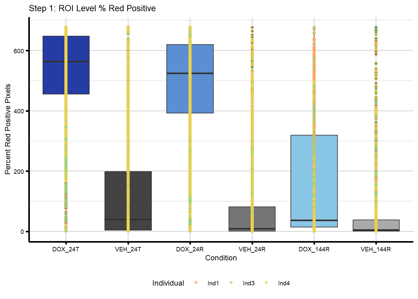
| Version | Author | Date |
|---|---|---|
| 0f7b54c | emmapfort | 2025-12-01 |
IF Quant Step 2
Collapse ROIs into an image level summary.
Read in Image Level Summary
#now that I've created the image level summary table for all individuals above, read it in so I don't have to create it multiple times

roi_image_level_summary <- readRDS("data/Fig1/IF_quant/roi_image_level_summary_all.RDS")
Make a Metadata Table
Combine Metadata with Image Level Summary
IF Quant Step 2
Collapse ROIs into their respective images.
#now I'll plot the outcome of the second step where I collapsed by image and merged the metadata with the measurements

plot_step2 <- ggplot(merged_image_summary,
         aes(x = Condition,
             y = Mean_Red_Positive_Pixels)) +
  geom_boxplot(aes(fill = Condition), show.legend = FALSE) +
  geom_point(aes(color = Individual),
             alpha = 0.8, #for visibility as I collapse data down
             size = 3,
             position = position_identity()) +
  scale_x_discrete(limits = condition_levels) +
  scale_color_manual(values = c(ind_cols_if)) +
  scale_fill_manual(values = txtime_col_old) +
  labs(title = "Step 2: Image-Level Mean Red Positive Pixels",
       x = "Condition",
       y = "Mean Red Positive Pixels") +
  theme_custom() +
  theme(legend.position = "bottom")


plot_step2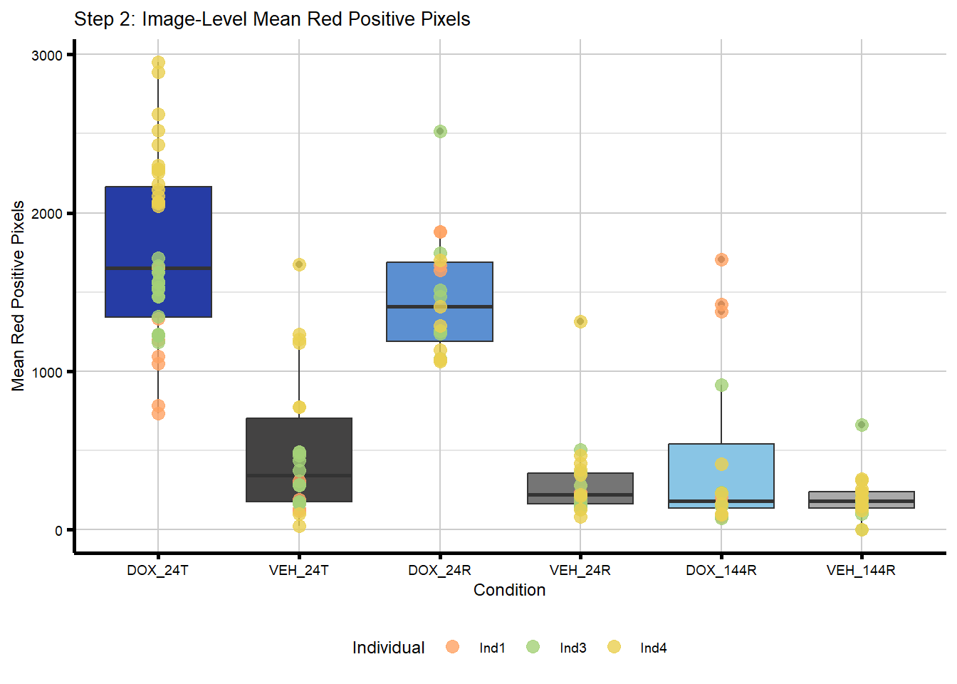
| Version | Author | Date |
|---|---|---|
| 0f7b54c | emmapfort | 2025-12-01 |
IF Quant Step 3
Select 3 images with consistent numbers of nuclei per individual.
#now I will be selecting images based on their nuclei count

#first let's find the median number of nuclei per individual to get an idea of how many are there per experiment
#all experiments were performed separately but with the same protocol, so each individual is separate

# median_nuclei <- merged_image_summary %>%
#   group_by(Individual, Condition) %>%
#   summarize(
#     Median_Nuclei = median(Nuclei_Count, na.rm = TRUE),
#     Mean_Positive = mean(Mean_Red_Positive_Pixels),
#     Image_Count = n(),
#     .groups = "drop"
#   ) %>%
#   arrange(Individual, Condition)

#let's pick out the three images per condition that have consistent nuclei counts

#first I am going to remove some outlier images from my Ind1 since I had some dim/blurry ones that should not be included since they weren't properly detected
#I chose the images that were in focus and had consistent numbers of nuclei based on summary from above

# Define the good images for Ind4 (IDs = the 4-digit part before "_DAPI")
# images_Ind4 <- tibble::tribble(
#   ~Condition,   ~ID,
#   "DOX_24T",  "0012",
#   "DOX_24T",  "0013",
#   "DOX_24T",  "0017",
#   "VEH_24T",  "0006",
#   "VEH_24T",  "0004",
#   "VEH_24T",  "0003",
#   "DOX_24R",  "0006",
#   "DOX_24R",  "0004",
#   "DOX_24R",  "0003",
#   "VEH_24R",  "0004",
#   "VEH_24R",  "0005",
#   "VEH_24R",  "0003",
#   "DOX_144R", "0002",
#   "DOX_144R", "0003",
#   "DOX_144R", "0005",
#   "VEH_144R", "0003",
#   "VEH_144R", "0004",
#   "VEH_144R", "0012"
# )

#filter my merged_image_summary for Ind1 using IDs
# ind4_filtered <- merged_image_summary %>%
#   filter(Individual == "Ind4") %>%
#   mutate(
#     Image_ID  = str_extract(Image, "_\\d{4}_") %>% str_remove_all("_")
#   ) %>%
#   inner_join(images_Ind1, by = c("Condition", "Image_ID" = "ID"))

#now join this back into my pipeline because now I have the images I need based on nucleus count?

# merged_image_summary_filt <- merged_image_summary %>%
#   dplyr::filter(Individual != "Ind4") %>%
#   bind_rows(ind1_filtered)

#now that I've put Ind1 back in, let's select images based on nuclei for Ind1 and Ind3

# select_top3_images <- function(df, individual) {
#   df %>%
#     filter(Individual == individual) %>%
#     group_by(Condition) %>%
#     mutate(
#       med_nuclei = median(Nuclei_Count, na.rm = TRUE),
#       med_pos    = median(Mean_Norm_Percent_Red_Positive, na.rm = TRUE),
#       score = abs(Nuclei_Count - med_nuclei) + abs(Mean_Norm_Percent_Red_Positive - med_pos)
#     ) %>%
#     arrange(score) %>%
#     slice_head(n = 3) %>%
#     ungroup()
# }

# ind1_filtered <- select_top3_images(merged_image_summary, "Ind1")
# ind3_filtered <- select_top3_images(merged_image_summary, "Ind3")

#filter Ind 4 to get the same scores at the end
# ind4_filtered <- ind4_filtered %>%
#     group_by(Condition) %>%
#     mutate(
#         med_nuclei = median(Nuclei_Count, na.rm = TRUE),
#         med_pos    = median(Mean_Percent_Red_Positive, na.rm = TRUE),
#         score = abs(Nuclei_Count - med_nuclei) +
#             abs(Mean_Percent_Red_Positive - med_pos)
#     ) %>%
#     ungroup()

#merge these summaries together to have all individuals represented in one
# merged_image_summary_final <- bind_rows(
#   merged_image_summary %>% filter(!Individual %in% c("Ind1", "Ind3", "Ind4")),
#   ind1_filtered,
#   ind3_filtered,
#   ind4_filtered
# ) %>%
#   dplyr::select(-("Image_ID"))

#save the finalized version as an R object and read it back in, keep code for posterity
# saveRDS(merged_image_summary_final, "data/Fig1/IF_quant/merged_image_summary_final.RDS")

merged_image_summary_final <- readRDS("data/Fig1/IF_quant/merged_image_summary_final.RDS")

#plot these in a boxplot now that they're filtered down to the top 3 images per individual based on consistent nuclei counts

plot_step3 <- ggplot(merged_image_summary_final,
                     aes(x = Condition,
                         y = Mean_Norm_Percent_Red_Positive)) +
  geom_boxplot(aes(fill = Condition), show.legend = FALSE) +
  geom_point(aes(color = Individual),
             size = 2,
             alpha = 1, #now fewer points so no need to be transparent
             position = position_identity()) +
  scale_x_discrete(limits = condition_levels) +
  scale_color_manual(values = c(ind_cols_if)) +
  scale_fill_manual(values = txtime_col_old) +
  labs(title = "Step 3: Select 3 Images Per Individual with Consistent Nuclei",
       x = "Condition",
       y = "Mean Percent Red Positive") +
  theme_custom() +
  theme(legend.position = "bottom")

plot_step3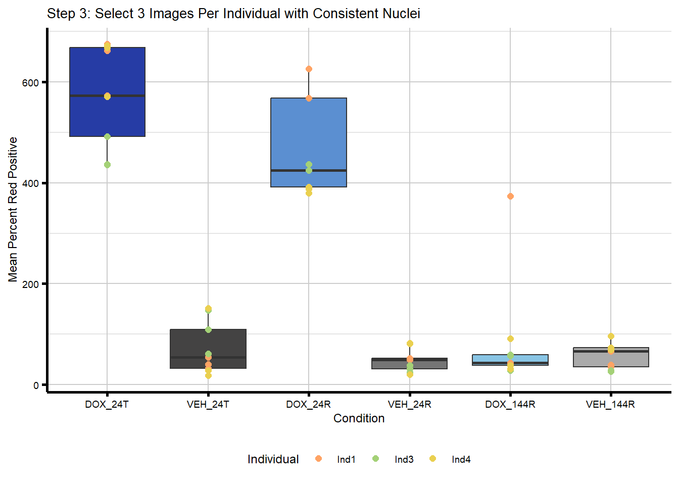
| Version | Author | Date |
|---|---|---|
| 0f7b54c | emmapfort | 2025-12-01 |
#do stats for step 3 boxplot between DOX and VEH at each timepoint for comparison
ttests_step3 <- merged_image_summary_final %>%
  group_by(Timepoint) %>%
  t_test(Mean_Norm_Percent_Red_Positive ~ Treatment) %>%
  mutate(
    y.position = max(merged_image_summary_final$Mean_Norm_Percent_Red_Positive, na.rm = TRUE) * 1.05
  )

sig_table_step3 <- merged_image_summary_final %>%
  group_by(Timepoint) %>%
  summarise(
    p = t.test(Mean_Norm_Percent_Red_Positive ~ Treatment)$p.value,
    y.position = max(Mean_Norm_Percent_Red_Positive, na.rm = TRUE) * 1.05,
    .groups = "drop"
  ) %>%
  mutate(
    signif = case_when(
      p < 0.001 ~ "***",
      p < 0.01  ~ "**",
      p < 0.05  ~ "*",
      TRUE      ~ "ns"
    ),
    group1 = paste0("VEH_", Timepoint),
    group2 = paste0("DOX_", Timepoint)
  )

ttests_step3
# A tibble: 3 × 10
Timepoint .y. group1 group2 n1 n2 statistic df p y.position
<chr> <chr> <chr> <chr> <int> <int> <dbl> <dbl> <dbl> <dbl>
1 144R Mean_N… DOX VEH 9 9 0.751 8.81 4.72e-1 708.
2 24R Mean_N… DOX VEH 9 9 11.8 8.72 1.20e-6 708.
3 24T Mean_N… DOX VEH 9 9 13.4 11.9 1.57e-8 708.#plot with t test statistics included above plot
plot_step3_test <- ggplot(merged_image_summary_final,
aes(x = Condition,
y = Mean_Norm_Percent_Red_Positive)) +
geom_boxplot(aes(fill = Condition), show.legend = FALSE) +
geom_point(aes(color = Individual),
size = 2,
alpha = 1,
position = position_identity()) +
stat_pvalue_manual(sig_table_step3,
label = "signif",
tip.length = 0.02) +
scale_x_discrete(limits = condition_levels) +
scale_color_manual(values = c(ind_cols_if)) +
scale_fill_manual(values = txtime_col_old) +
labs(title = "Step 3: Select 3 Images Per Individual with Consistent Nuclei",
x = "Condition",
y = "Mean Percent Red Positive") +
theme_custom() +
theme(legend.position = "bottom")
plot_step3_test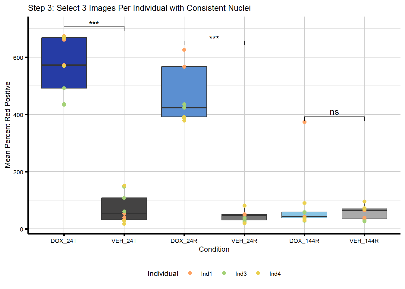
| Version | Author | Date |
|---|---|---|
| 0f7b54c | emmapfort | 2025-12-01 |
IF Quant Step 4
Normalize DOX/VEH before combining images by individual.
#Now I want to normalize these images by max intensity

merged_image_summary_norm <- merged_image_summary_final %>%
  group_by(Magnification) %>%
  mutate(Norm_Percent_Red_Positive = (Mean_Percent_Red_Positive / max(Mean_Percent_Red_Positive, na.rm = TRUE)) * 100) %>%
  ungroup() %>%
  mutate(Condition = paste0(Treatment, "_", Timepoint))

#now these are scaled 0-100

individual_summary_norm <- merged_image_summary_norm %>%
  group_by(Individual, Treatment, Timepoint) %>%
  summarise(
    Mean_Norm = mean(Norm_Percent_Red_Positive, na.rm = TRUE),
    Median_Norm = median(Norm_Percent_Red_Positive, na.rm = TRUE),
    .groups = "drop"
  ) %>%
  mutate(
    Condition = paste0(Treatment, "_", Timepoint)
  )

#alter the t test table from before to plot the same comparisons
ttest_table_step4 <- ttests_step3 %>%
  filter(Timepoint %in% c("24T", "24R", "144R")) %>%
  mutate(
    group1 = paste0("DOX_", Timepoint),
    group2 = paste0("VEH_", Timepoint),
    y.position = max(individual_summary_norm$Mean_Norm, na.rm = TRUE) * 1.05,

    #add in significance stars
    p.signif = case_when(
      p < 0.001 ~ "***",
      p < 0.01  ~ "**",
      p < 0.05  ~ "*",
      TRUE      ~ "ns"
    )
  )

#plot step 4
plot_step4 <- ggplot(merged_image_summary_norm,
                     aes(x = Condition,
                         y = Norm_Percent_Red_Positive)) +
  geom_boxplot(aes(fill = Condition), show.legend = FALSE) +
  geom_point(aes(color = Individual),
             size = 2,
             alpha = 1,
             position = position_identity()) +
  scale_y_continuous(limits = c(0, 105)) +
  scale_x_discrete(limits = condition_levels) +
  scale_color_manual(values = ind_cols_if) +
  scale_fill_manual(values = txtime_col_old) +
  stat_pvalue_manual(ttest_table_step4,
                     label = "p.signif",
                     xmin = "group1",
                     xmax = "group2",
                     tip.length = 0.02) +
  labs(title = "Step 4: Normalized by Max Intensity (0–100%)",
       x = "Condition",
       y = "Percent Red Positive") +
  theme_custom() +
  theme(legend.position = "bottom")

plot_step4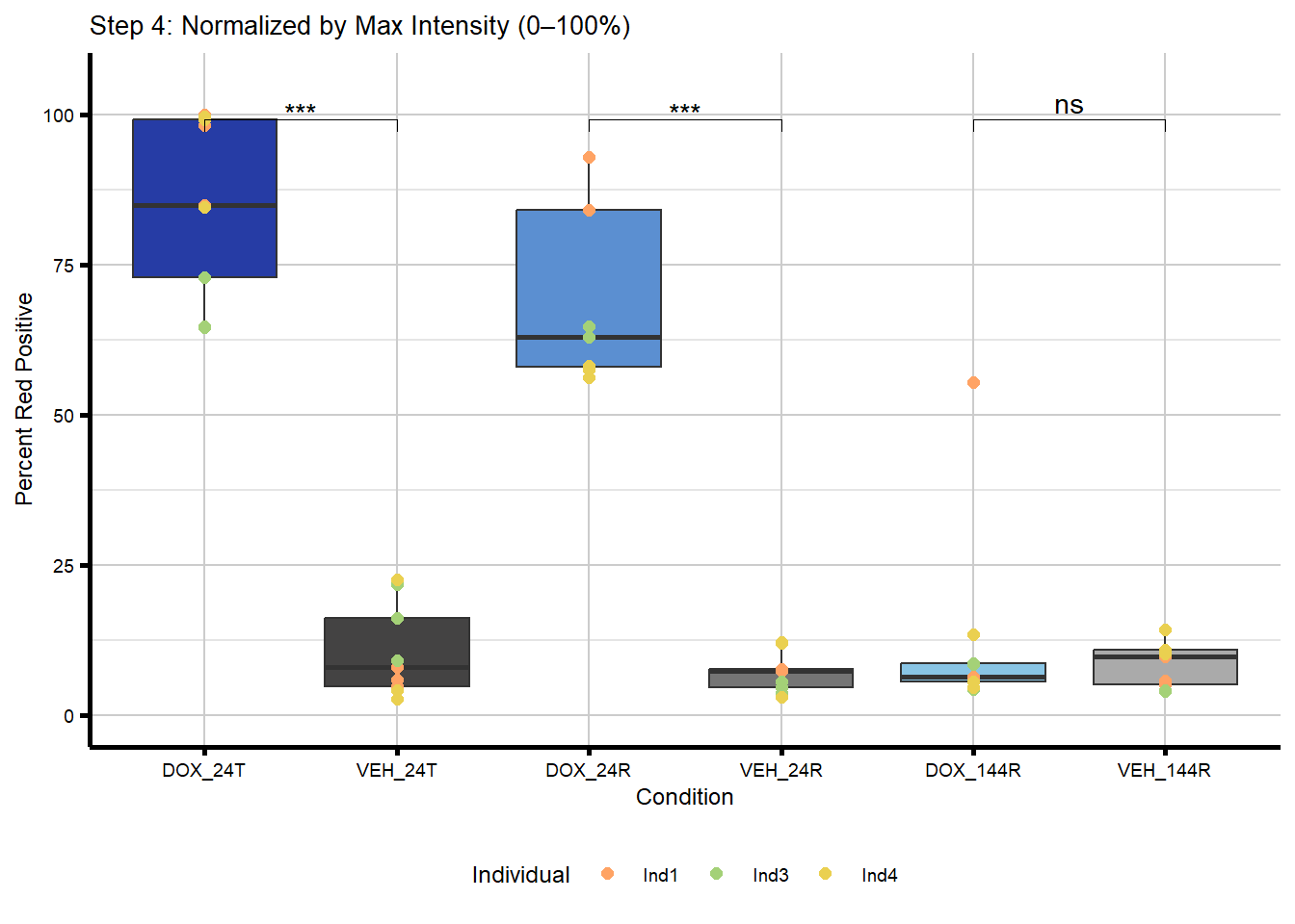
| Version | Author | Date |
|---|---|---|
| 0f7b54c | emmapfort | 2025-12-01 |
IF Quant Step 5
Collapse images by individual.
#now I want to collapse these three images per condition into their respective individual after normalization
#I now only have three points, one per individual, on each boxplot
#I also performed a t-test between DOX and VEH at each timepoint to assess differences between treated and untreated within each timepoint

individual_summary_step5 <- merged_image_summary_norm %>%
  group_by(Individual, Treatment, Timepoint, Magnification) %>%
  summarise(
    Mean_Norm = mean(Norm_Percent_Red_Positive, na.rm = TRUE),
    Median_Norm = median(Norm_Percent_Red_Positive, na.rm = TRUE),
    .groups = "drop"
  ) %>%
  mutate(
    Condition = paste0(Treatment, "_", Timepoint)
  )

#utilize the same t tests performed earlier since it is just a collapsed version of the same data
#changed the name to reduce confusion
ttest_table_step5 <- ttests_step3 %>%
  filter(Timepoint %in% c("24T", "24R", "144R")) %>%
  mutate(
    group1 = paste0("DOX_", Timepoint),
    group2 = paste0("VEH_", Timepoint),
    y.position = max(individual_summary_step5$Mean_Norm, na.rm = TRUE) * 1.05,

    #add in significance stars
    p.signif = case_when(
      p < 0.001 ~ "***",
      p < 0.01  ~ "**",
      p < 0.05  ~ "*",
      TRUE      ~ "ns"
    )
  )


#plot the collapsed image-level data 0-100
plot_step5 <- ggplot(individual_summary_step5,
                     aes(x = Condition, y = Mean_Norm)) +
  geom_boxplot(aes(fill = Condition), show.legend = FALSE) +
  geom_point(aes(color = Individual),
             size = 3,
             alpha = 1,
             position = position_identity()) +
  scale_y_continuous(limits = c(0, 100)) +
  scale_x_discrete(limits = condition_levels) +
  scale_color_manual(values = ind_cols_if) +
  scale_fill_manual(values = txtime_col_old) +
  stat_pvalue_manual(ttest_table_step5,
                     label = "p.signif",
                     xmin = "group1",
                     xmax = "group2",
                     tip.length = 0.02) +
  labs(title = "Step 5: Individual-Level Percent Red Positive",
       x = "Condition",
       y = "Normalized Percent Positive") +
  theme_custom() +
  theme(legend.position = "bottom")

plot_step5
Warning in grid.Call(C_textBounds, as.graphicsAnnot(x$label), x$x, x$y, : font
family not found in Windows font database
Warning in grid.Call(C_textBounds, as.graphicsAnnot(x$label), x$x, x$y, : font
family not found in Windows font database
Warning in grid.Call(C_textBounds, as.graphicsAnnot(x$label), x$x, x$y, : font
family not found in Windows font database
Warning in grid.Call(C_textBounds, as.graphicsAnnot(x$label), x$x, x$y, : font
family not found in Windows font databaseWarning in grid.Call.graphics(C_text, as.graphicsAnnot(x$label), x$x, x$y, :
font family not found in Windows font database
Warning in grid.Call.graphics(C_text, as.graphicsAnnot(x$label), x$x, x$y, :
font family not found in Windows font database
Warning in grid.Call.graphics(C_text, as.graphicsAnnot(x$label), x$x, x$y, :
font family not found in Windows font database
Warning in grid.Call.graphics(C_text, as.graphicsAnnot(x$label), x$x, x$y, :
font family not found in Windows font database
Warning in grid.Call.graphics(C_text, as.graphicsAnnot(x$label), x$x, x$y, :
font family not found in Windows font database
Warning in grid.Call.graphics(C_text, as.graphicsAnnot(x$label), x$x, x$y, :
font family not found in Windows font database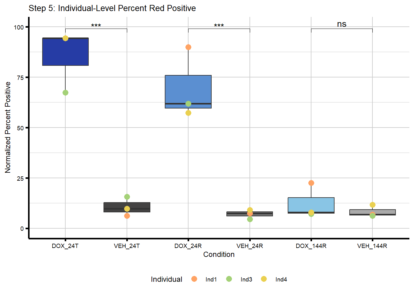
| Version | Author | Date |
|---|---|---|
| 0f7b54c | emmapfort | 2025-12-01 |
# save_plot(
#   plot = plot_step5,
#   filename = "IFQuant_Step5_Final_EMP",
#   folder = output_folder,
#   height = plot_height,
#   width = plot_width
# )
IF Quant Step 6
Perform significance testing between treated timepoints.
#Above, I compared DOX to VEH for each timepoint
#I want to now make comparisons between DOX timepoints to see if there are any differences between each timepoint after treatment and recovery time
#I will then add these to the plot in Illustrator to show both comparisons together since they don't want to plot correctly

individual_summary_step6_dox <- merged_image_summary_norm %>%
  group_by(Individual, Treatment, Timepoint, Magnification) %>%
  summarise(
    Mean_Norm = mean(Norm_Percent_Red_Positive, na.rm = TRUE),
    Median_Norm = median(Norm_Percent_Red_Positive, na.rm = TRUE),
    .groups = "drop"
  ) %>%
  mutate(
    Condition = paste0(Treatment, "_", Timepoint)
  )

#set condition levels for x axis to plot all boxes
condition_levels <- c("DOX_24T", "VEH_24T",
                      "DOX_24R", "VEH_24R",
                      "DOX_144R", "VEH_144R")

dox_conditions <- c("DOX_24T", "DOX_24R", "DOX_144R")

individual_summary_step6_dox <- individual_summary_step6_dox %>%
  mutate(Condition = factor(Condition, levels = condition_levels))

#perform paired t-tests between DOX timepoints
timepoint_pairs <- list(
  c("24T","24R"),
  c("24R","144R"),
  c("24T","144R")
)

#t test table
ttest_table_dox_time <- purrr::map_df(seq_along(timepoint_pairs), function(i){
  tp <- timepoint_pairs[[i]]

  df_wide <- individual_summary_step6_dox %>%
    filter(Timepoint %in% tp) %>%
    group_by(Individual, Timepoint) %>%
    summarise(Mean_Norm = mean(Mean_Norm, na.rm = TRUE), .groups = "drop") %>%
    pivot_wider(names_from = Timepoint, values_from = Mean_Norm) %>%
    drop_na()

  base_y <- max(individual_summary_step6_dox$Mean_Norm,
                na.rm = TRUE) * 0.9

  y_increment <- max(individual_summary_step6_dox$Mean_Norm,
                     na.rm = TRUE) * 0.05

  y_pos <- base_y + y_increment * i

  if(nrow(df_wide) < 2){
    tibble(
      group1 = paste0("DOX_", tp[1]),
      group2 = paste0("DOX_", tp[2]),
      p.value = NA_real_,
      p.signif = "NA",
      y.position = y_pos
    )
  } else {
    test <- t.test(df_wide[[tp[1]]], df_wide[[tp[2]]], paired = TRUE)
    tibble(
      group1 = paste0("DOX_", tp[1]),
      group2 = paste0("DOX_", tp[2]),
      p.value = test$p.value,
      p.signif = case_when(
        test$p.value < 0.001 ~ "***",
        test$p.value < 0.01  ~ "**",
        test$p.value < 0.05  ~ "*",
        TRUE                 ~ "ns"
      ),
      y.position = y_pos
    )
  }
})

#map to numeric positions for stat_pvalue_manual
ttest_table_dox_time <- ttest_table_dox_time %>%
  mutate(
    group1_num = as.numeric(factor(group1, levels = condition_levels)),
    group2_num = as.numeric(factor(group2, levels = condition_levels))
  )

#manually set y positions for each comparison (so I can see all of it)
max_val <- max(individual_summary_step6_dox$Mean_Norm, na.rm = TRUE)

ttest_table_dox_time <- ttest_table_dox_time %>%
  mutate(
    y.position = case_when(
      group1 == "DOX_24T" & group2 == "DOX_24R" ~ max_val * 1.05,  #middle
      group1 == "DOX_24T" & group2 == "DOX_144R" ~ max_val * 1.10, #top
      group1 == "DOX_24R" & group2 == "DOX_144R" ~ max_val * 1.00  #bottom
    ),
    group1_num = as.numeric(factor(group1, levels = condition_levels)),
    group2_num = as.numeric(factor(group2, levels = condition_levels))
  )

#plot DOX timepoint comparisons
plot_step6_dox_time <- ggplot(individual_summary_step6_dox,
                              aes(x = Condition,
                                  y = Mean_Norm)) +
  geom_boxplot(aes(fill = Condition),
               show.legend = FALSE) +
  geom_point(aes(color = Individual),
             size = 3,
             alpha = 1,
             position = position_identity()) +
  scale_y_continuous(limits = c(0, 105)) +
  scale_x_discrete(limits = condition_levels) +
  scale_color_manual(values = ind_cols_if) +
  scale_fill_manual(values = txtime_col_old) +
  stat_pvalue_manual(ttest_table_dox_time,
                     label = "p.signif",
                     xmin = "group1_num",
                     xmax = "group2_num",
                     y.position = "y.position",
                     tip.length = 0.02) +
  labs(title = "Step 6: DOX Timepoint Comparisons Norm Percent Positive",
       x = "Condition",
       y = "Normalized Percent Positive") +
  theme_custom() +
  theme(legend.position = "bottom")

#print the plot
plot_step6_dox_time
Warning in grid.Call(C_textBounds, as.graphicsAnnot(x$label), x$x, x$y, : font
family not found in Windows font database
Warning in grid.Call(C_textBounds, as.graphicsAnnot(x$label), x$x, x$y, : font
family not found in Windows font database
Warning in grid.Call(C_textBounds, as.graphicsAnnot(x$label), x$x, x$y, : font
family not found in Windows font database
Warning in grid.Call(C_textBounds, as.graphicsAnnot(x$label), x$x, x$y, : font
family not found in Windows font databaseWarning in grid.Call.graphics(C_text, as.graphicsAnnot(x$label), x$x, x$y, :
font family not found in Windows font database
Warning in grid.Call.graphics(C_text, as.graphicsAnnot(x$label), x$x, x$y, :
font family not found in Windows font database
Warning in grid.Call.graphics(C_text, as.graphicsAnnot(x$label), x$x, x$y, :
font family not found in Windows font database
Warning in grid.Call.graphics(C_text, as.graphicsAnnot(x$label), x$x, x$y, :
font family not found in Windows font database
Warning in grid.Call.graphics(C_text, as.graphicsAnnot(x$label), x$x, x$y, :
font family not found in Windows font database
Warning in grid.Call.graphics(C_text, as.graphicsAnnot(x$label), x$x, x$y, :
font family not found in Windows font database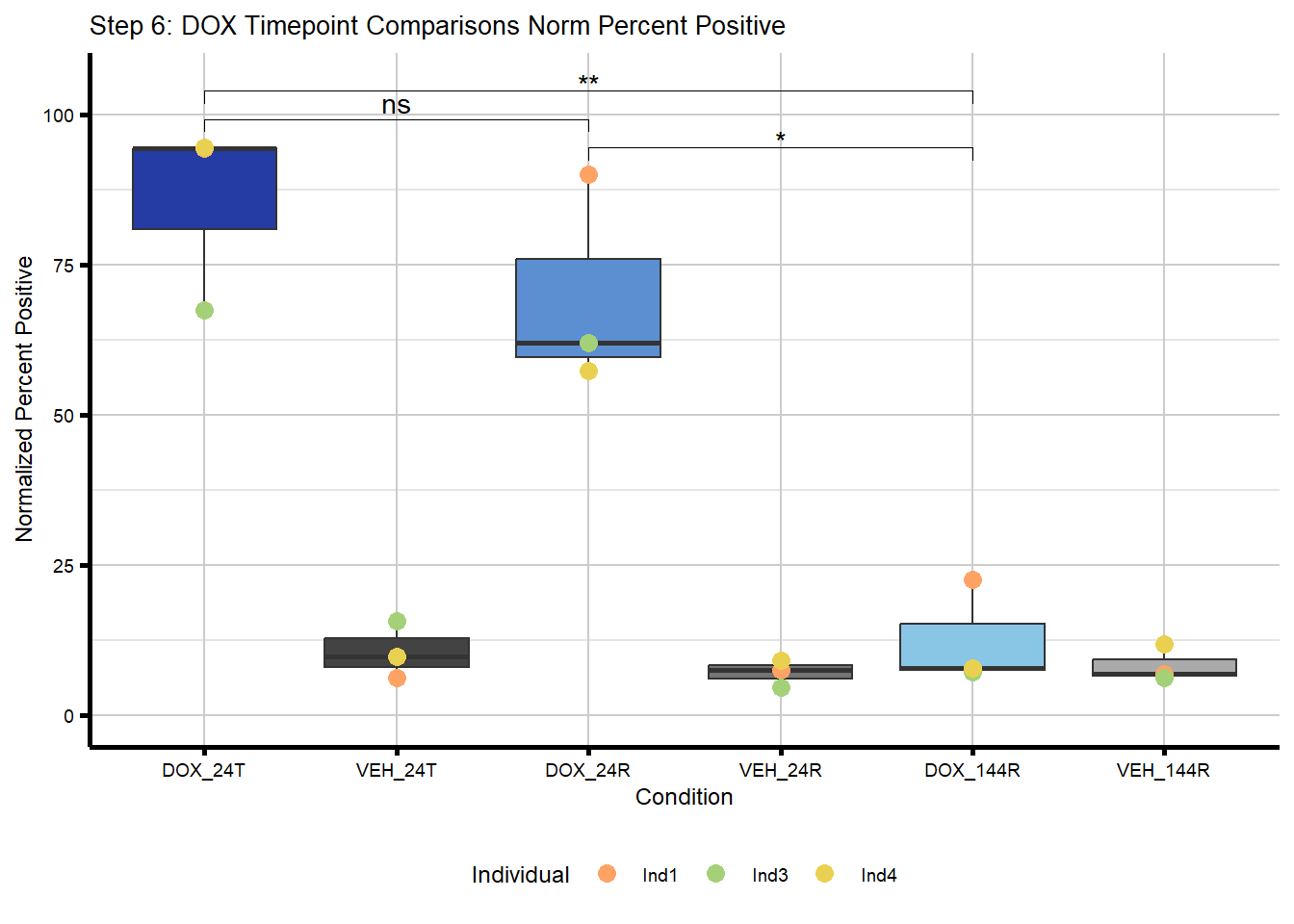
| Version | Author | Date |
|---|---|---|
| 0f7b54c | emmapfort | 2025-12-01 |
# save_plot(
#   plot = plot_step6_dox_time,
#   filename = "IFQuant_Step6_DOX_TimeComp_EMP",
#   folder = output_folder
# )
Figure 1E - yH2AX IF Images (no code)
Images from individual 87-1 (Ind1).
sessionInfo()R version 4.4.2 (2024-10-31 ucrt)
Platform: x86_64-w64-mingw32/x64
Running under: Windows 11 x64 (build 22000)
Matrix products: default
locale:
[1] LC_COLLATE=English_United States.utf8
[2] LC_CTYPE=English_United States.utf8
[3] LC_MONETARY=English_United States.utf8
[4] LC_NUMERIC=C
[5] LC_TIME=English_United States.utf8
time zone: America/Chicago
tzcode source: internal
attached base packages:
[1] stats graphics grDevices utils datasets methods base
other attached packages:
[1] ggpubr_0.6.0 rstatix_0.7.2 RImageJROI_0.1.3 scales_1.4.0
[5] drc_3.0-1 MASS_7.3-61 readxl_1.4.5 lubridate_1.9.4
[9] forcats_1.0.0 stringr_1.5.1 dplyr_1.1.4 purrr_1.0.4
[13] readr_2.1.5 tidyr_1.3.1 tibble_3.2.1 ggplot2_3.5.2
[17] tidyverse_2.0.0 workflowr_1.7.1
loaded via a namespace (and not attached):
[1] tidyselect_1.2.1 farver_2.1.2 fastmap_1.2.0
[4] TH.data_1.1-3 spatstat.geom_3.5-0 promises_1.3.2
[7] digest_0.6.37 timechange_0.3.0 lifecycle_1.0.4
[10] survival_3.7-0 processx_3.8.6 spatstat.data_3.1-6
[13] magrittr_2.0.3 compiler_4.4.2 rlang_1.1.6
[16] sass_0.4.10 tools_4.4.2 utf8_1.2.5
[19] plotrix_3.8-4 yaml_2.3.10 ggsignif_0.6.4
[22] knitr_1.50 labeling_0.4.3 bit_4.5.0
[25] RColorBrewer_1.1-3 multcomp_1.4-28 abind_1.4-8
[28] withr_3.0.2 grid_4.4.2 polyclip_1.10-7
[31] git2r_0.36.2 gtools_3.9.5 spatstat.utils_3.1-5
[34] cli_3.6.3 mvtnorm_1.3-3 crayon_1.5.3
[37] rmarkdown_2.29 generics_0.1.4 rstudioapi_0.17.1
[40] httr_1.4.7 tzdb_0.5.0 cachem_1.1.0
[43] splines_4.4.2 parallel_4.4.2 cellranger_1.1.0
[46] vctrs_0.6.5 Matrix_1.7-1 sandwich_3.1-1
[49] jsonlite_2.0.0 carData_3.0-5 car_3.1-3
[52] callr_3.7.6 hms_1.1.3 bit64_4.5.2
[55] Formula_1.2-5 spatstat.univar_3.1-4 jquerylib_0.1.4
[58] glue_1.8.0 codetools_0.2-20 ps_1.9.1
[61] stringi_1.8.7 gtable_0.3.6 later_1.4.2
[64] deldir_2.0-4 pillar_1.10.2 htmltools_0.5.8.1
[67] R6_2.6.1 rprojroot_2.0.4 vroom_1.6.5
[70] evaluate_1.0.3 lattice_0.22-6 backports_1.5.0
[73] broom_1.0.8 httpuv_1.6.16 bslib_0.9.0
[76] Rcpp_1.0.14 whisker_0.4.1 xfun_0.52
[79] fs_1.6.6 zoo_1.8-14 getPass_0.2-4
[82] pkgconfig_2.0.3