Figure 5 Analysis
Last updated: 2026-01-06
Checks: 7 0
Knit directory: DXR_website/
This reproducible R Markdown analysis was created with workflowr (version 1.7.1). The Checks tab describes the reproducibility checks that were applied when the results were created. The Past versions tab lists the development history.
Great! Since the R Markdown file has been committed to the Git repository, you know the exact version of the code that produced these results.
Great job! The global environment was empty. Objects defined in the global environment can affect the analysis in your R Markdown file in unknown ways. For reproduciblity it’s best to always run the code in an empty environment.
The command set.seed(20251201) was run prior to running
the code in the R Markdown file. Setting a seed ensures that any results
that rely on randomness, e.g. subsampling or permutations, are
reproducible.
Great job! Recording the operating system, R version, and package versions is critical for reproducibility.
Nice! There were no cached chunks for this analysis, so you can be confident that you successfully produced the results during this run.
Great job! Using relative paths to the files within your workflowr project makes it easier to run your code on other machines.
Great! You are using Git for version control. Tracking code development and connecting the code version to the results is critical for reproducibility.
The results in this page were generated with repository version cd535e9. See the Past versions tab to see a history of the changes made to the R Markdown and HTML files.
Note that you need to be careful to ensure that all relevant files for
the analysis have been committed to Git prior to generating the results
(you can use wflow_publish or
wflow_git_commit). workflowr only checks the R Markdown
file, but you know if there are other scripts or data files that it
depends on. Below is the status of the Git repository when the results
were generated:
Ignored files:
    Ignored:    .Rhistory
    Ignored:    .Rproj.user/
    Ignored:    DXR_website/data/
    Ignored:    code/Flow_Purity_Stressor_Boxplots_EMP_250226.R
    Ignored:    data/CDKN1A_geneplot_Dox.RDS
    Ignored:    data/Cormotif_dox.RDS
    Ignored:    data/Cormotif_prob_gene_list.RDS
    Ignored:    data/Cormotif_prob_gene_list_doxonly.RDS
    Ignored:    data/Counts_RNA_EMPfortmiller.txt
    Ignored:    data/DMSO_TNN13_plot.RDS
    Ignored:    data/DOX_TNN13_plot.RDS
    Ignored:    data/DOXgeneplots.RDS
    Ignored:    data/ExpressionMatrix_EMP.csv
    Ignored:    data/Ind1_DOX_Spearman_plot.RDS
    Ignored:    data/Ind6REP_Spearman_list.csv
    Ignored:    data/Ind6REP_Spearman_plot.RDS
    Ignored:    data/Ind6REP_Spearman_set.csv
    Ignored:    data/Ind6_Spearman_plot.RDS
    Ignored:    data/MDM2_geneplot_Dox.RDS
    Ignored:    data/Master_summary_75-1_EMP_250811_final.csv
    Ignored:    data/Master_summary_87-1_EMP_250811_final.csv
    Ignored:    data/Metadata.csv
    Ignored:    data/Metadata_2_norep_update.RDS
    Ignored:    data/Metadata_update.csv
    Ignored:    data/QC/
    Ignored:    data/Recovery_flow_purity.csv
    Ignored:    data/SIRT1_geneplot_Dox.RDS
    Ignored:    data/Sample_annotated.csv
    Ignored:    data/SpearmanHeatmapMatrix_EMP
    Ignored:    data/VolcanoPlot_D144R_original_EMP_250623.png
    Ignored:    data/VolcanoPlot_D24R_original_EMP_250623.png
    Ignored:    data/VolcanoPlot_D24T_original_EMP_250623.png
    Ignored:    data/annot_dox.RDS
    Ignored:    data/annot_list_hm.csv
    Ignored:    data/cormotif_dxr_1.RDS
    Ignored:    data/cormotif_dxr_2.RDS
    Ignored:    data/counts/
    Ignored:    data/counts_DE_df_dox.RDS
    Ignored:    data/counts_DE_raw_data.RDS
    Ignored:    data/counts_raw_filt.RDS
    Ignored:    data/counts_raw_matrix.RDS
    Ignored:    data/counts_raw_matrix_EMP_250514.csv
    Ignored:    data/d24_Spearman_plot.RDS
    Ignored:    data/dge_calc_dxr.RDS
    Ignored:    data/dge_calc_matrix.RDS
    Ignored:    data/ensembl_backup_dox.RDS
    Ignored:    data/fC_AllCounts.RDS
    Ignored:    data/fC_DOXCounts.RDS
    Ignored:    data/featureCounts_Concat_Matrix_DOXSamples_EMP_250430.csv
    Ignored:    data/featureCounts_DOXdata_updatedind.RDS
    Ignored:    data/filcpm_colnames_matrix.csv
    Ignored:    data/filcpm_matrix.csv
    Ignored:    data/filt_gene_list_dox.RDS
    Ignored:    data/filter_gene_list_final.RDS
    Ignored:    data/final_data/
    Ignored:    data/gene_clustlike_motif.RDS
    Ignored:    data/gene_postprob_motif.RDS
    Ignored:    data/genedf_dxr.RDS
    Ignored:    data/genematrix_dox.RDS
    Ignored:    data/genematrix_dxr.RDS
    Ignored:    data/heartgenes.csv
    Ignored:    data/heartgenes_dox.csv
    Ignored:    data/image_intensity_stats_all_conditions.csv
    Ignored:    data/image_level_stats_all_conditions.csv
    Ignored:    data/image_level_summary_yH2AX_quant.csv
    Ignored:    data/ind_num_dox.RDS
    Ignored:    data/ind_num_dxr.RDS
    Ignored:    data/initial_cormotif.RDS
    Ignored:    data/initial_cormotif_dox.RDS
    Ignored:    data/low_nuclei_samples.csv
    Ignored:    data/low_veh_samples.csv
    Ignored:    data/new/
    Ignored:    data/new_cormotif_dox.RDS
    Ignored:    data/perc_mean_all_10X.png
    Ignored:    data/perc_mean_all_20X.png
    Ignored:    data/perc_mean_all_40X.png
    Ignored:    data/perc_mean_consistent_10X.png
    Ignored:    data/perc_mean_consistent_20X.png
    Ignored:    data/perc_mean_consistent_40X.png
    Ignored:    data/perc_median_all_10X.png
    Ignored:    data/perc_median_all_20X.png
    Ignored:    data/perc_median_all_40X.png
    Ignored:    data/perc_median_consistent_10X.png
    Ignored:    data/perc_median_consistent_20X.png
    Ignored:    data/perc_median_consistent_40X.png
    Ignored:    data/plot_leg_d.RDS
    Ignored:    data/plot_leg_d_horizontal.RDS
    Ignored:    data/plot_leg_d_vertical.RDS
    Ignored:    data/plot_theme_custom.RDS
    Ignored:    data/process_gene_data_funct.RDS
    Ignored:    data/raw_mean_all_10X.png
    Ignored:    data/raw_mean_all_20X.png
    Ignored:    data/raw_mean_all_40X.png
    Ignored:    data/raw_mean_consistent_10X.png
    Ignored:    data/raw_mean_consistent_20X.png
    Ignored:    data/raw_mean_consistent_40X.png
    Ignored:    data/raw_median_all_10X.png
    Ignored:    data/raw_median_all_20X.png
    Ignored:    data/raw_median_all_40X.png
    Ignored:    data/raw_median_consistent_10X.png
    Ignored:    data/raw_median_consistent_20X.png
    Ignored:    data/raw_median_consistent_40X.png
    Ignored:    data/ruv/
    Ignored:    data/summary_all_IF_ROI.RDS
    Ignored:    data/tableED_GOBP.RDS
    Ignored:    data/tableESR_GOBP_postprob.RDS
    Ignored:    data/tableLD_GOBP.RDS
    Ignored:    data/tableLR_GOBP_postprob.RDS
    Ignored:    data/tableNR_GOBP.RDS
    Ignored:    data/tableNR_GOBP_postprob.RDS
    Ignored:    data/table_incsus_genes_GOBP_RUV.RDS
    Ignored:    data/table_motif1_GOBP_d.RDS
    Ignored:    data/table_motif1_genes_GOBP.RDS
    Ignored:    data/table_motif2_GOBP_d.RDS
    Ignored:    data/table_motif3_genes_GOBP.RDS
    Ignored:    data/thing.R
    Ignored:    data/top.table_V.D144r_dox.RDS
    Ignored:    data/top.table_V.D24_dox.RDS
    Ignored:    data/top.table_V.D24r_dox.RDS
    Ignored:    data/yH2AX_75-1_EMP_250811.csv
    Ignored:    data/yH2AX_87-1_EMP_250811.csv
    Ignored:    data/yH2AX_Boxplots_MeanIntensity_10X_EMP_250811.png
    Ignored:    data/yH2AX_Boxplots_MeanIntensity_10X_NormtoMax_EMP_250811.png
    Ignored:    data/yH2AX_Boxplots_MeanIntensity_20X_EMP_250811.png
    Ignored:    data/yH2AX_Boxplots_MeanIntensity_20X_NormtoMax_EMP_250811.png
    Ignored:    data/yH2AX_Boxplots_MedianIntensity_10X_NormtoMax_EMP_250811.png
    Ignored:    data/yH2AX_Boxplots_MedianIntensity_20X_NormtoMax_EMP_250811.png
    Ignored:    data/yH2AX_Boxplots_MedianIntensity_NormtoMax_EMP_250811.png
    Ignored:    data/yH2AX_Boxplots_Quant_10X_EMP_250817.png
    Ignored:    data/yH2AX_Boxplots_Quant_20X_EMP_250817.png
    Ignored:    data/yh2ax_all_df_EMP_250812.csv

Unstaged changes:
    Modified:   analysis/DXR_Project_Analysis.Rmd
Note that any generated files, e.g. HTML, png, CSS, etc., are not included in this status report because it is ok for generated content to have uncommitted changes.
These are the previous versions of the repository in which changes were
made to the R Markdown (DXR_website/analysis/Figure5.Rmd)
and HTML (DXR_website/docs/Figure5.html) files. If you’ve
configured a remote Git repository (see ?wflow_git_remote),
click on the hyperlinks in the table below to view the files as they
were in that past version.
| File | Version | Author | Date | Message |
|---|---|---|---|---|
| Rmd | cd535e9 | emmapfort | 2026-01-06 | Final Website Touches 01/06/25 EMP |
| html | 7f22593 | emmapfort | 2026-01-05 | Build site. |
| Rmd | 49fa865 | emmapfort | 2026-01-05 | Final Updates to Website EMP 01/05/26 |
| Rmd | da1f69c | emmapfort | 2025-12-02 | updated analysis 12/02/25 |
Libraries
Load necessary libraries for analysis.
library(tidyverse)
library(readxl)
library(readr)
library(ComplexHeatmap)
library(reshape2)
library(circlize)
library(grid)
library(stringr)
library(org.Hs.eg.db)
library(AnnotationDbi)
Define my custom plot theme
# Define the custom theme
# plot_theme_custom <- function() {
#   theme_minimal() +
#     theme(
#       #line for x and y axis
#       axis.line = element_line(linewidth = 1,
#                                color = "black"),
#
#       #axis ticks only on x and y, length standard
#       axis.ticks.x = element_line(color = "black",
#                                 linewidth = 1),
#       axis.ticks.y = element_line(color = "black",
#                                 linewidth = 1),
#       axis.ticks.length = unit(0.05, "in"),
#
#       #text and font
#       axis.text = element_text(color = "black",
#                                family = "Arial",
#                                size = 7),
#       axis.title = element_text(color = "black",
#                                 family = "Arial",
#                                 size = 9),
#       legend.text = element_text(color = "black",
#                                  family = "Arial",
#                                  size = 7),
#       legend.title = element_text(color = "black",
#                                   family = "Arial",
#                                   size = 9),
#       plot.title = element_text(color = "black",
#                                 family = "Arial",
#                                 size = 10),
#
#       #blank background and border
#       panel.background = element_blank(),
#       panel.border = element_blank(),
#
#       #gridlines for alignment
#       panel.grid.major = element_line(color = "grey80", linewidth = 0.5),  #grey major grid for align in illus
#       panel.grid.minor = element_line(color = "grey90", linewidth = 0.5) #grey minor grid for align in illus
#     )
# }

# saveRDS(plot_theme_custom, "data/plot_theme_custom.RDS")

theme_custom <- readRDS("data/plot_theme_custom.RDS")
Define a function to save plots as .pdf and .png
save_plot <- function(plot, filename,
                      folder = ".",
                      width = 8,
                      height = 6,
                      units = "in",
                      dpi = 300,
                      add_date = TRUE) {
  if (missing(filename)) stop("Please provide a filename (without extension) for the plot.")

  date_str <- if (add_date) paste0("_", format(Sys.Date(), "%y%m%d")) else ""
  pdf_file <- file.path(folder, paste0(filename, date_str, ".pdf"))
  png_file <- file.path(folder, paste0(filename, date_str, ".png"))
  ggsave(filename = pdf_file, plot = plot, device = cairo_pdf, width = width, height = height, units = units, bg = "transparent")
  ggsave(filename = png_file, plot = plot, device = "png", width = width, height = height, units = units, dpi = dpi, bg = "transparent")
  message("Saved plot as Cairo PDF: ", pdf_file)
  message("Saved plot as PNG: ", png_file)
}

output_folder <- "C:/Users/emmap/OneDrive/Desktop/DXR Manuscript Materials/Fig pdfs"


#save plot function created
#to use: just define the plot name, filename_base, width, height
Read in Gene Lists from Literature
I utilized gene sets from two additional studies - a p53 target gene set (Fischer, M., Census and evaluation of p53 target genes. Oncogene, 2017. 36(28): p. 3943-3956) and a DNA damage response (DDR) gene set (Liberzon, A., et al., The Molecular Signatures Database (MSigDB) hallmark gene set collection. Cell Syst, 2015. 1(6): p. 417-425).
#DDR gene set from Liberzon et al.

#read in my DDR gene set
DNA_damage <- readRDS("data/Fig5/DNA_damage_response_genes.RDS")

#pull out only the unique values that are not NA (there aren't any)
ddr_set <- unique(na.omit(DNA_damage))
#pull out the entrez ids
entrezids_DDR_R <- unname(DNA_damage)
#calculate the total length of my gene set for proportion analysis
total_ddr_genes <- length(ddr_set)
cat("Total DNA damage genes:", total_ddr_genes, "\n")
Total DNA damage genes: 65 #should be 65 total genes
#p53 target genes from Fischer et al.
p53_target_genes <- readRDS("data/Fig5/p53_target_genes_list.RDS")
#pull out only the unique values that are not NA (there aren't any)
p53_set <- unique(na.omit(p53_target_genes))
#pull out the entrez ids
entrezids_p53 <- unname(p53_set)
#calculate the total length of my gene set for proportion analysis
total_p53_genes <- length(p53_set)
cat("Total p53 Target genes:", total_p53_genes, "\n")Total p53 Target genes: 300 Figure 5A - Forest Plot of Odds Ratios
#define my gene clusters

final_genes_1_RUV <- readRDS("data/Fig3/final_genes_1_RUV.RDS")
final_genes_2_RUV <- readRDS("data/Fig3/final_genes_2_RUV.RDS")

motifs <- list(
  acute = final_genes_1_RUV,
  chronic = final_genes_2_RUV
)

#define the gene sets from above to test with a Fisher's exact test between clusters
gene_sets <- list(
  DDR = ddr_set,
  P53 = p53_set
)

#all tested genes as background
all_genes <- readRDS("data/DE/all_genes.RDS")

#compare between motif clusters for acute and chronic
compare_motifs <- function(acute, chronic, gene_set, gene_set_name) {
  in_chronic <- sum(chronic %in% gene_set)
  out_chronic <- length(chronic) - in_chronic
  in_acute <- sum(acute %in% gene_set)
  out_acute <- length(acute) - in_acute

  mat <- matrix(c(in_chronic, out_chronic, in_acute, out_acute), nrow = 2, byrow = TRUE)
  rownames(mat) <- c("Chronic", "Acute")
  colnames(mat) <- c("In_Set", "Not_In_Set")

  test <- fisher.test(mat)

  tibble(
    Gene_Set = gene_set_name,
    Motif_Comparison = "Chronic_vs_Acute",
    In_Set_Chronic = in_chronic,
    In_Set_Acute = in_acute,
    Odds_Ratio = as.numeric(test$estimate),
    CI_Low = test$conf.int[1],
    CI_High = test$conf.int[2],
    P_Value = test$p.value
  )
}

#apply for each gene set
comparison_results <- map_dfr(names(gene_sets), function(gs_name) {
  compare_motifs(final_genes_1_RUV, final_genes_2_RUV, gene_sets[[gs_name]], gs_name)
})

print(comparison_results)
# A tibble: 2 × 8
Gene_Set Motif_Comparison In_Set_Chronic In_Set_Acute Odds_Ratio CI_Low
<chr> <chr> <int> <int> <dbl> <dbl>
1 DDR Chronic_vs_Acute 16 24 10.4 5.13
2 P53 Chronic_vs_Acute 28 170 2.59 1.65
# ℹ 2 more variables: CI_High <dbl>, P_Value <dbl>#add sigificance and percent overlap
comparison_results <- comparison_results %>%
mutate(
Perc_Chronic = round((In_Set_Chronic / length(final_genes_2_RUV)) * 100, 2),
Perc_Acute = round((In_Set_Acute / length(final_genes_1_RUV)) * 100, 2),
Significance = case_when(
P_Value < 0.001 ~ "***",
P_Value < 0.01 ~ "**",
P_Value < 0.05 ~ "*",
TRUE ~ ""
),
Odds_Ratio = round(Odds_Ratio, 3),
CI_Low = round(CI_Low, 3),
CI_High = round(CI_High, 3),
P_Value = signif(P_Value, 3)
)
#create a final summary table
summary_table <- comparison_results %>%
dplyr::select(
Gene_Set,
In_Set_Chronic, Perc_Chronic,
In_Set_Acute, Perc_Acute,
Odds_Ratio, CI_Low, CI_High, P_Value, Significance
)
cat("\n--- Chronic vs Acute Enrichment Summary ---\n")
--- Chronic vs Acute Enrichment Summary ---print(summary_table)# A tibble: 2 × 10
Gene_Set In_Set_Chronic Perc_Chronic In_Set_Acute Perc_Acute Odds_Ratio CI_Low
<chr> <int> <dbl> <int> <dbl> <dbl> <dbl>
1 DDR 16 3.19 24 0.32 10.4 5.13
2 P53 28 5.59 170 2.24 2.59 1.65
# ℹ 3 more variables: CI_High <dbl>, P_Value <dbl>, Significance <chr>#now create a forest plot
p_comparison <- ggplot(comparison_results,
aes(y = Gene_Set, x = Odds_Ratio,
xmin = CI_Low, xmax = CI_High)) +
geom_point(size = 4) +
geom_errorbarh(height = 0.1, size = 1, color = "black") +
geom_text(aes(label = Significance),
position = position_nudge(y = 0.2),
color = "black", fontface = "bold", size = 5) +
geom_vline(xintercept = 1, linetype = "dashed", color = "red") +
scale_x_log10(limits = c(1, 30),
breaks = c(1, 10, 20)) +
labs(
x = "log odds ratio (95% confidence interval)",
y = NULL,
title = "Enrichment of DDR + p53 target genes Chronic vs Acute",
) +
theme_custom()
print(p_comparison)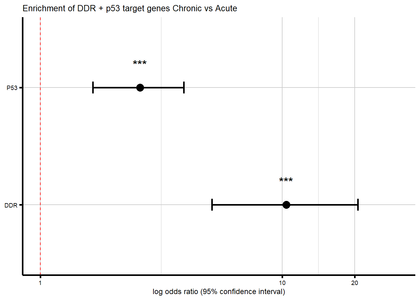
| Version | Author | Date |
|---|---|---|
| 7f22593 | emmapfort | 2026-01-05 |
Figure 5B - log2FC Heatmap DDR tx+144 DEGs
#load in DEGs for all timepoints
DOX_24T_R <- read.csv("data/DE/Toptable_RUV_24T_final.csv") %>%
  dplyr::select(-(X))
DOX_24R_R <- read.csv("data/DE/Toptable_RUV_24R_final.csv") %>%
  dplyr::select(-(X))
DOX_144R_R <- read.csv("data/DE/Toptable_RUV_144R_final.csv") %>%
  dplyr::select(-(X))

#extract Significant DEGs from these lists
DEGs_24T_R <- DOX_24T_R$Entrez_ID[DOX_24T_R$adj.P.Val < 0.05]
DEGs_24R_R <- DOX_24R_R$Entrez_ID[DOX_24R_R$adj.P.Val < 0.05]
DEGs_144R_R <- DOX_144R_R$Entrez_ID[DOX_144R_R$adj.P.Val < 0.05]


#DDR Entrez_ID and categories
entrez_category_DDR <- tribble(
  ~ENTREZID, ~Category,
  317, "Apoptosis", 355, "Apoptosis", 581, "Apoptosis", 637, "Apoptosis",
  836, "Apoptosis", 841, "Apoptosis", 842, "Apoptosis", 27113, "Apoptosis",
  5366, "Apoptosis", 54205, "Apoptosis", 55367, "Apoptosis", 8795, "Apoptosis",
  1026, "Cell Cycle / Checkpoint", 1027, "Cell Cycle / Checkpoint", 595, "Cell Cycle / Checkpoint",
  894, "Cell Cycle / Checkpoint", 896, "Cell Cycle / Checkpoint", 898, "Cell Cycle / Checkpoint",
  9133, "Cell Cycle / Checkpoint", 9134, "Cell Cycle / Checkpoint", 891, "Cell Cycle / Checkpoint",
  983, "Cell Cycle / Checkpoint", 1017, "Cell Cycle / Checkpoint", 1019, "Cell Cycle / Checkpoint",
  1020, "Cell Cycle / Checkpoint", 1021, "Cell Cycle / Checkpoint", 993, "Cell Cycle / Checkpoint",
  995, "Cell Cycle / Checkpoint", 1869, "Cell Cycle / Checkpoint", 4609, "Cell Cycle / Checkpoint",
  5925, "Cell Cycle / Checkpoint", 9874, "Cell Cycle / Checkpoint", 11011, "Cell Cycle / Checkpoint",
  1385, "Cell Cycle / Checkpoint",
  472, "Damage Sensors / Signal Transducers", 545, "Damage Sensors / Signal Transducers",
  5591, "Damage Sensors / Signal Transducers", 5810, "Damage Sensors / Signal Transducers",
  5883, "Damage Sensors / Signal Transducers", 5884, "Damage Sensors / Signal Transducers",
  6118, "Damage Sensors / Signal Transducers", 4361, "Damage Sensors / Signal Transducers",
  10111, "Damage Sensors / Signal Transducers", 4683, "Damage Sensors / Signal Transducers",
  84126, "Damage Sensors / Signal Transducers", 3014, "Damage Sensors / Signal Transducers",
  672, "DNA Repair", 2177, "DNA Repair", 5888, "DNA Repair", 5893, "DNA Repair",
  1647, "DNA Repair", 4616, "DNA Repair", 10912, "DNA Repair", 1111, "DNA Repair",
  11200, "DNA Repair", 1643, "DNA Repair", 8243, "DNA Repair", 5981, "DNA Repair",
  7157, "p53 Regulators / Targets", 4193, "p53 Regulators / Targets", 5371, "p53 Regulators / Targets",
  27244, "p53 Regulators / Targets", 50484, "p53 Regulators / Targets",
  207, "Miscellaneous / Broad", 25, "Miscellaneous / Broad"
)

entrez_ids_DDR_R <- entrez_category_DDR$ENTREZID


#function to extract relevant data
extract_data_DDR_RUV <- function(df, name) {
  df %>%
    filter(Entrez_ID %in% entrez_ids_DDR_R) %>%
    mutate(Gene = mapIds(org.Hs.eg.db,
                         as.character(Entrez_ID),
                         column = "SYMBOL",
                         keytype = "ENTREZID",
                         multiVals = "first"),
           Condition = name,
           Signif = ifelse(adj.P.Val < 0.05, "*", ""))
}


#DEG list
deg_list_RUV <- list("t0" = DOX_24T_R,
                 "t24" = DOX_24R_R,
                 "t144" = DOX_144R_R
)

#combine all DEGs and annotate
all_data_DDR_RUV <- bind_rows(mapply(extract_data_DDR_RUV, deg_list_RUV, names(deg_list_RUV), SIMPLIFY = FALSE))

#now make a filtering step to only include DEGs at tx+144
sig_genes_t144 <- all_data_DDR_RUV %>%
  dplyr::filter(Condition == "t144", adj.P.Val < 0.05) %>%
  pull(Gene) %>%
  unique()

filt_DDR_data_t144 <- all_data_DDR_RUV %>%
  dplyr::filter(Gene %in% sig_genes_t144)

#create matrices
logFC_mat_DDR_RUV <- acast(filt_DDR_data_t144, Gene ~ Condition, value.var = "logFC")
signif_mat_DDR_RUV <- acast(filt_DDR_data_t144, Gene ~ Condition, value.var = "Signif")

#desired column order
desired_order <- c("t0",
                   "t24",
                   "t144")

logFC_mat_DDR_RUV <- logFC_mat_DDR_RUV[, desired_order]
signif_mat_DDR_RUV <- signif_mat_DDR_RUV[, desired_order]

#column annotation
meta_DDR_RUV <- str_split_fixed(colnames(logFC_mat_DDR_RUV), "_", 2)
timepoint_annot <- colnames(logFC_mat_DDR_RUV)
col_annot_DDR_RUV <- HeatmapAnnotation(
  Timepoint = timepoint_annot,
  col = list(
    Timepoint = c("t0" = "#005A4C",
                  "t24" = "#328477",
                  "t144" = "#8FB9B1")
  ),
  annotation_height = unit(c(1, 1, 1), "cm"),
  annotation_legend_param = list(
    Timepoint = list(
      at = c("t0", "t24", "t144")
    )
  )
)

#draw heatmap
ddr_hm_5b <- Heatmap(logFC_mat_DDR_RUV,
        name = "log2FC",
        top_annotation = col_annot_DDR_RUV,
        cluster_columns = FALSE,
        cluster_rows = FALSE,
        show_row_names = TRUE,
        row_names_gp = gpar(fontsize = 7),
        show_column_names = FALSE,
        column_names_gp = gpar(fontsize = 7),
        rect_gp = gpar(col = "black", lwd = 0.5),
        border = gpar(col = "black"),
        layer_fun = function(j, i, x, y, width, height, fill) {
          grid.text(signif_mat_DDR_RUV[cbind(i, j)], x, y, gp = gpar(fontsize = 12))
        },
        column_title = "DDR gene response (Liberzon et al.)",
        column_title_gp = gpar(fontsize = 9, fontface = "plain"),
        heatmap_legend_param = list(
          title_gp = gpar(fontsize = 8, fontface = "plain"),
          labels_gp = gpar(fontsize = 7, fontface = "plain")
  )
)

print(ddr_hm_5b)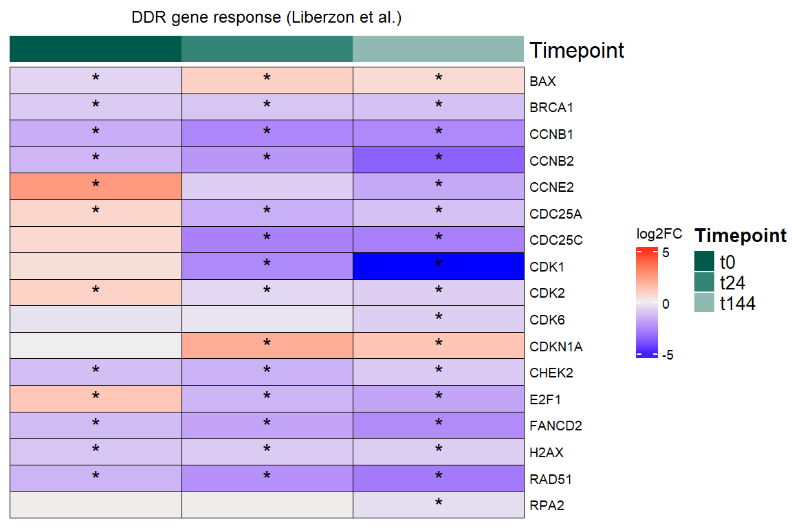
| Version | Author | Date |
|---|---|---|
| 7f22593 | emmapfort | 2026-01-05 |
#make a function to save complex heatmaps
save_complex_heatmap <- function(plot, filename, folder, width = 6, height = 8) {
  if (!dir.exists(folder)) dir.create(folder, recursive = TRUE)
    path <- file.path(folder, filename)
    pdf(path, width = width, height = height)
    draw(plot, heatmap_legend_side = "right")
    dev.off()
  message("Saved heatmap to: ", path)
}

#save to PDF in your output folder
# save_complex_heatmap(
#   plot = ddr_hm_5b,
#   filename = "Fig5B_logFCHM_RUV_DDR_EMP.pdf",
#   folder = output_folder,
#   width = 8,
#   height = 7
# )
Figure 5C - p53 Target Genes logFC Heatmap
#use DEGs above

#p53 target Entrez_ID
entrez_ids_p53 <- c(1026,50484,4193,9766,9518,7832,1643,1647,1263,57103,51065,8795,51499,64393,581,
                5228,5429,8493,55959,7508,64782,282991,355,53836,4814,10769,9050,27244,9540,94241,
                26154,57763,900,26999,55332,26263,23479,23612,29950,9618,10346,8824,134147,55294,
                22824,4254,6560,467,27113,60492,8444,60401,1969,220965,2232,3976,55191,84284,93129,
                5564,7803,83667,7779,132671,7039,51768,137695,93134,7633,10973,340485,307,27350,
                23245,3732,29965,1363,1435,196513,8507,8061,2517,51278,53354,54858,23228,5366,5912,
                6236,51222,26152,59,1907,50650,91012,780,9249,11072,144455,64787,116151,27165,2876,
                57822,55733,57722,121457,375449,85377,4851,5875,127544,29901,84958,8797,8793,441631,
                220001,54541,5889,5054,25816,25987,5111,98,317,598,604,10904,1294,80315,53944,
                1606,2770,3628,3675,3985,4035,4163,84552,29085,55367,5371,5791,54884,5980,8794,
                1462,50808,220,583,694,1056,9076,10978,54677,1612,55040,114907,2274,127707,4000,
                8079,4646,4747,27445,5143,80055,79156,5360,5364,23654,5565,5613,5625,10076,56963,
                6004,390,255488,6326,6330,23513,7869,283130,204962,83959,6548,6774,9263,10228,
                22954,10475,85363,494514,10142,79714,1006,8446,9648,79828,5507,55240,63874,25841,
                9289,84883,154810,51321,421,8553,655,119032,84280,10950,824,839,57828,857,8812,
                8837,94027,113189,22837,132864,10898,3300,81704,1847,1849,1947,9538,24139,5168,
                147965,115548,9873,23768,2632,2817,3280,3265,23308,3490,51477,182,3856,8844,144811,
                9404,4043,9848,2872,23041,740,343263,4638,26509,4792,22861,57523,55214,80025,164091,
                57060,64065,51090,5453,8496,333926,55671,5900,55544,23179,8601,389,6223,55800,6385,
                4088,6643,122809,257397,285343,7011,54790,374618,55362,51754,7157,9537,22906,7205,
                80705,219699,55245,83719,7748,25946,118738)


#function to extract relevant data
extract_data_p53_RUV <- function(df, name) {
  df %>%
    filter(Entrez_ID %in% entrez_ids_p53) %>%
    mutate(Gene = mapIds(org.Hs.eg.db,
                         as.character(Entrez_ID),
                         column = "SYMBOL",
                         keytype = "ENTREZID",
                         multiVals = "first"),
           Condition = name,
           Signif = ifelse(adj.P.Val < 0.05, "*", ""))
}

#DEG list
deg_list_RUV <- list("t0" = DOX_24T_R,
                 "t24" = DOX_24R_R,
                 "t144" = DOX_144R_R
)

#combine all DEGs and annotate
all_data_p53_RUV <- bind_rows(mapply(extract_data_p53_RUV, deg_list_RUV,
                                     names(deg_list_RUV), SIMPLIFY = FALSE))

#now make a filtering step to only include DEGs at tx+144
sig_genes_t144 <- all_data_p53_RUV %>%
  dplyr::filter(Condition == "t144", adj.P.Val < 0.05) %>%
  pull(Gene) %>%
  unique()

filt_p53_data_t144 <- all_data_p53_RUV %>%
  dplyr::filter(Gene %in% sig_genes_t144)

#create matrices
logFC_mat53_RUV <- acast(filt_p53_data_t144, Gene ~ Condition, value.var = "logFC")
signif_mat53_RUV <- acast(filt_p53_data_t144, Gene ~ Condition, value.var = "Signif")

#desired column order
desired_order <- c("t0",
                   "t24",
                   "t144")

logFC_mat_p53_RUV <- logFC_mat53_RUV[, desired_order]
signif_mat_p53_RUV <- signif_mat53_RUV[, desired_order]

#column annotation
timepoint_annot <- colnames(logFC_mat_p53_RUV)

col_annot_p53_RUV <- HeatmapAnnotation(
  Timepoint = timepoint_annot,
  col = list(
    Timepoint = c("t0" = "#005A4C",
             "t24" = "#328477",
             "t144" = "#8FB9B1")
  ),
  annotation_height = unit(c(1, 1, 1), "cm"),
  annotation_legend_param = list(
    Timepoint = list(
      at = c("t0", "t24", "t144")
    )
  )
)

#draw heatmap
p53_hm_5c <- Heatmap(
  logFC_mat_p53_RUV,
  name = "log2FC",
  top_annotation = col_annot_p53_RUV,
  cluster_columns = FALSE,
  cluster_rows = TRUE,
  show_row_names = TRUE,
  row_names_gp = gpar(fontsize = 7),
  show_column_names = FALSE,
  column_names_gp = gpar(fontsize = 7),
  rect_gp = gpar(col = "black", lwd = 0.5),
  border = "black",
  layer_fun = function(j, i, x, y, width, height, fill) {
    grid.text(signif_mat_p53_RUV[cbind(i, j)], x, y, gp = gpar(fontsize = 12))
  },
  column_title = "p53 gene response (Fischer et al.)",
  column_title_gp = gpar(fontsize = 9, fontface = "plain"),
  heatmap_legend_param = list(
          title_gp = gpar(fontsize = 8, fontface = "plain"),
          labels_gp = gpar(fontsize = 7)
  )
)

print(p53_hm_5c)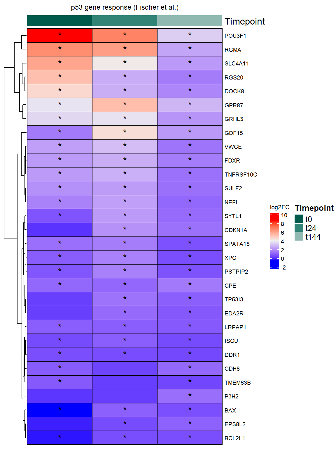
| Version | Author | Date |
|---|---|---|
| 7f22593 | emmapfort | 2026-01-05 |
Supplementary Figure 8A - DDR target gene enrichment in DEGs vs nonDEGs
#DEGs list
timepoint_DEGs_ddr <- list(
  "t0"   = DEGs_24T_R,
  "t24"   = DEGs_24R_R,
  "t144"  = DEGs_144R_R
)

#calculate proportions, odds ratios, and Fisher's test results per timepoint
proportion_data_ddr <- purrr::map_dfr(names(timepoint_DEGs_ddr), function(tp_ddr) {
  degs_ddr <- unique(timepoint_DEGs_ddr[[tp_ddr]])
  nondegs_ddr <- setdiff(all_genes, degs_ddr)

  in_deg_ddr <- sum(degs_ddr %in% ddr_set)
  in_deg_nonddr <- length(degs_ddr) - in_deg_ddr

  in_nondeg_ddr <- sum(nondegs_ddr %in% ddr_set)
  in_nondeg_nonddr <- length(nondegs_ddr) - in_nondeg_ddr

  contingency_degs_ddr <- matrix(c(in_deg_ddr, in_deg_nonddr,
                                   in_nondeg_ddr, in_nondeg_nonddr),
                                 nrow = 2, byrow = TRUE)

  fisher_res_ddr <- fisher.test(contingency_degs_ddr)

  p_val_ddr <- fisher_res_ddr$p.value
  odds_ratio_ddr <- unname(fisher_res_ddr$estimate)
  ci_low_ddr <- fisher_res_ddr$conf.int[1]
  ci_high_ddr <- fisher_res_ddr$conf.int[2]

  tibble(
    Timepoint = tp_ddr,
    Odds_Ratio = odds_ratio_ddr,
    CI_low = ci_low_ddr,
    CI_high = ci_high_ddr,
    P_Value = p_val_ddr,
    Significant = p_val_ddr < 0.05
  )
})

# Format Timepoint factor and add significance label/color
proportion_data_ddr <- proportion_data_ddr %>%
  mutate(
    Timepoint = factor(Timepoint, levels = c("t0", "t24", "t144")),
    Sig_Label = ifelse(Significant, "Significant", "Not Significant")
  )

#plot horizontal forest plot
supp8_forest_ddr_A <- ggplot(proportion_data_ddr, aes(y = Timepoint, x = Odds_Ratio, color = Sig_Label)) +
  geom_point(size = 5) +
  geom_errorbarh(aes(xmin = CI_low, xmax = CI_high), height = 0.3) +
  geom_vline(xintercept = 1, linetype = "dashed", color = "gray50") +
  scale_color_manual(values = c("Significant" = "black", "Not Significant" = "pink")) +
  scale_x_log10() +
  labs(
    title = "Odds Ratios of DDR Gene Enrichment by Timepoint",
    y = "Timepoint",
    x = "Odds Ratio (log scale)",
    color = "Significance"
  ) +
  scale_y_discrete(limits = rev(levels(proportion_data_ddr$Timepoint)))+
  theme_custom()

print(supp8_forest_ddr_A)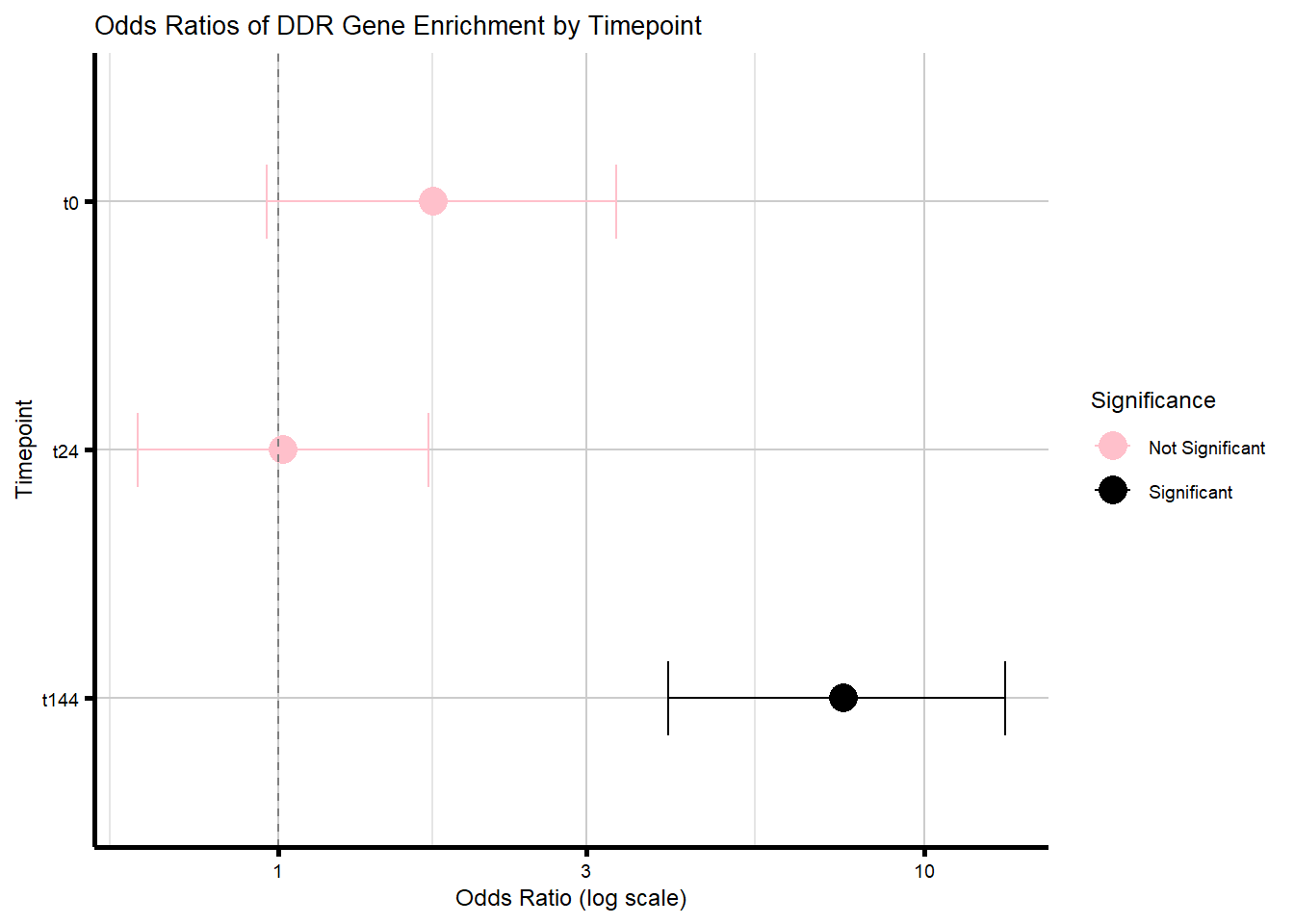
| Version | Author | Date |
|---|---|---|
| 7f22593 | emmapfort | 2026-01-05 |
# save_plot(
#   plot = supp8_forest_ddr_A,
#   filename = "Supp8_ForestDDR_EMP",
#   folder = output_folder,
#   height = 4,
#   width = 6)
Supplementary Figure 8B - p53 target gene enrichment in DEGs vs nonDEGs
timepoint_DEGs_p53 <- list(
  "t0"   = DEGs_24T_R,
  "t24"   = DEGs_24R_R,
  "t144"  = DEGs_144R_R
)

proportion_data_p53 <- purrr::map_dfr(names(timepoint_DEGs_p53), function(tp_p53) {
  degs_p53 <- unique(timepoint_DEGs_p53[[tp_p53]])
  nondegs_p53 <- setdiff(all_genes, degs_p53)

  in_deg_p53 <- sum(degs_p53 %in% p53_set)
  in_deg_nonp53 <- length(degs_p53) - in_deg_p53

  in_nondeg_p53 <- sum(nondegs_p53 %in% p53_set)
  in_nondeg_nonp53 <- length(nondegs_p53) - in_nondeg_p53

  contingency_degs_p53 <- matrix(c(in_deg_p53, in_deg_nonp53,
                                   in_nondeg_p53, in_nondeg_nonp53),
                                 nrow = 2, byrow = TRUE)

  fisher_res_p53 <- fisher.test(contingency_degs_p53)

  p_val_p53 <- fisher_res_p53$p.value
  odds_ratio_p53 <- unname(fisher_res_p53$estimate)
  ci_low_p53 <- fisher_res_p53$conf.int[1]
  ci_high_p53 <- fisher_res_p53$conf.int[2]

  tibble(
    Timepoint = tp_p53,
    Odds_Ratio = odds_ratio_p53,
    CI_low = ci_low_p53,
    CI_high = ci_high_p53,
    P_Value = p_val_p53,
    Significant = p_val_p53 < 0.01
  )
})

# Format Timepoint factor and add significance label/color
proportion_data_p53 <- proportion_data_p53 %>%
  mutate(
    Timepoint = factor(Timepoint, levels = c("t0", "t24", "t144")),
    Sig_Label = ifelse(Significant, "Significant", "Not Significant")
  )

#plot horizontal forest plot with color by significance
supp8_forest_p53_B <- ggplot(proportion_data_p53, aes(y = Timepoint, x = Odds_Ratio, color = Sig_Label)) +
  geom_point(size = 5) +
  geom_errorbarh(aes(xmin = CI_low, xmax = CI_high), height = 0.3) +
  geom_vline(xintercept = 1, linetype = "dashed", color = "gray50") +
  scale_color_manual(values = c("Significant" = "black", "Not Significant" = "pink")) +
  scale_x_log10() +
  labs(
    title = "Odds Ratios of p53 Gene Enrichment by Timepoint",
    y = "Timepoint",
    x = "Odds Ratio (log scale)",
    color = "Significance"
  ) +
  scale_y_discrete(limits = rev(levels(proportion_data_p53$Timepoint)))+
  theme_custom()


print(supp8_forest_p53_B)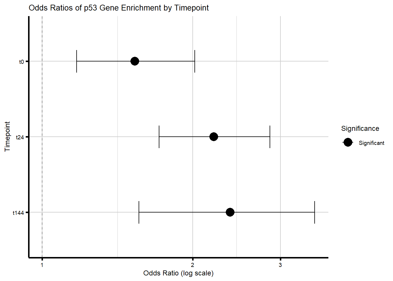
| Version | Author | Date |
|---|---|---|
| 7f22593 | emmapfort | 2026-01-05 |
# save_plot(
#   plot = supp8_forest_p53_B,
#   filename = "Supp8B_Forestp53_EMP",
#   folder = output_folder,
#   height = 4,
#   width = 6)
sessionInfo()R version 4.4.2 (2024-10-31 ucrt)
Platform: x86_64-w64-mingw32/x64
Running under: Windows 11 x64 (build 22000)
Matrix products: default
locale:
[1] LC_COLLATE=English_United States.utf8
[2] LC_CTYPE=English_United States.utf8
[3] LC_MONETARY=English_United States.utf8
[4] LC_NUMERIC=C
[5] LC_TIME=English_United States.utf8
time zone: America/Chicago
tzcode source: internal
attached base packages:
[1] stats4 grid stats graphics grDevices utils datasets
[8] methods base
other attached packages:
[1] org.Hs.eg.db_3.20.0 AnnotationDbi_1.68.0 IRanges_2.40.0
[4] S4Vectors_0.44.0 Biobase_2.66.0 BiocGenerics_0.52.0
[7] circlize_0.4.16 reshape2_1.4.4 ComplexHeatmap_2.22.0
[10] readxl_1.4.5 lubridate_1.9.4 forcats_1.0.0
[13] stringr_1.5.1 dplyr_1.1.4 purrr_1.0.4
[16] readr_2.1.5 tidyr_1.3.1 tibble_3.2.1
[19] ggplot2_3.5.2 tidyverse_2.0.0 workflowr_1.7.1
loaded via a namespace (and not attached):
[1] tidyselect_1.2.1 blob_1.2.4 farver_2.1.2
[4] Biostrings_2.74.0 fastmap_1.2.0 promises_1.3.2
[7] digest_0.6.37 timechange_0.3.0 lifecycle_1.0.4
[10] cluster_2.1.6 Cairo_1.6-5 KEGGREST_1.46.0
[13] processx_3.8.6 RSQLite_2.3.9 magrittr_2.0.3
[16] compiler_4.4.2 rlang_1.1.6 sass_0.4.10
[19] tools_4.4.2 utf8_1.2.5 yaml_2.3.10
[22] knitr_1.50 bit_4.5.0 plyr_1.8.9
[25] RColorBrewer_1.1-3 withr_3.0.2 git2r_0.36.2
[28] colorspace_2.1-1 scales_1.4.0 iterators_1.0.14
[31] cli_3.6.3 rmarkdown_2.29 crayon_1.5.3
[34] generics_0.1.4 rstudioapi_0.17.1 httr_1.4.7
[37] tzdb_0.5.0 rjson_0.2.23 DBI_1.2.3
[40] cachem_1.1.0 zlibbioc_1.52.0 parallel_4.4.2
[43] XVector_0.46.0 cellranger_1.1.0 matrixStats_1.5.0
[46] vctrs_0.6.5 jsonlite_2.0.0 callr_3.7.6
[49] hms_1.1.3 GetoptLong_1.0.5 bit64_4.5.2
[52] clue_0.3-66 magick_2.9.0 foreach_1.5.2
[55] jquerylib_0.1.4 glue_1.8.0 codetools_0.2-20
[58] ps_1.9.1 stringi_1.8.7 gtable_0.3.6
[61] shape_1.4.6.1 GenomeInfoDb_1.42.3 later_1.4.2
[64] UCSC.utils_1.2.0 pillar_1.10.2 htmltools_0.5.8.1
[67] GenomeInfoDbData_1.2.13 R6_2.6.1 doParallel_1.0.17
[70] rprojroot_2.0.4 evaluate_1.0.3 png_0.1-8
[73] memoise_2.0.1 httpuv_1.6.16 bslib_0.9.0
[76] Rcpp_1.0.14 whisker_0.4.1 xfun_0.52
[79] fs_1.6.6 getPass_0.2-4 pkgconfig_2.0.3
[82] GlobalOptions_0.1.2