Figure 7 Analysis
Last updated: 2026-01-06
Checks: 7 0
Knit directory: DXR_website/
This reproducible R Markdown analysis was created with workflowr (version 1.7.1). The Checks tab describes the reproducibility checks that were applied when the results were created. The Past versions tab lists the development history.
Great! Since the R Markdown file has been committed to the Git repository, you know the exact version of the code that produced these results.
Great job! The global environment was empty. Objects defined in the global environment can affect the analysis in your R Markdown file in unknown ways. For reproduciblity it’s best to always run the code in an empty environment.
The command set.seed(20251201) was run prior to running
the code in the R Markdown file. Setting a seed ensures that any results
that rely on randomness, e.g. subsampling or permutations, are
reproducible.
Great job! Recording the operating system, R version, and package versions is critical for reproducibility.
Nice! There were no cached chunks for this analysis, so you can be confident that you successfully produced the results during this run.
Great job! Using relative paths to the files within your workflowr project makes it easier to run your code on other machines.
Great! You are using Git for version control. Tracking code development and connecting the code version to the results is critical for reproducibility.
The results in this page were generated with repository version cd535e9. See the Past versions tab to see a history of the changes made to the R Markdown and HTML files.
Note that you need to be careful to ensure that all relevant files for
the analysis have been committed to Git prior to generating the results
(you can use wflow_publish or
wflow_git_commit). workflowr only checks the R Markdown
file, but you know if there are other scripts or data files that it
depends on. Below is the status of the Git repository when the results
were generated:
Ignored files:
    Ignored:    .Rhistory
    Ignored:    .Rproj.user/
    Ignored:    DXR_website/data/
    Ignored:    code/Flow_Purity_Stressor_Boxplots_EMP_250226.R
    Ignored:    data/CDKN1A_geneplot_Dox.RDS
    Ignored:    data/Cormotif_dox.RDS
    Ignored:    data/Cormotif_prob_gene_list.RDS
    Ignored:    data/Cormotif_prob_gene_list_doxonly.RDS
    Ignored:    data/Counts_RNA_EMPfortmiller.txt
    Ignored:    data/DMSO_TNN13_plot.RDS
    Ignored:    data/DOX_TNN13_plot.RDS
    Ignored:    data/DOXgeneplots.RDS
    Ignored:    data/ExpressionMatrix_EMP.csv
    Ignored:    data/Ind1_DOX_Spearman_plot.RDS
    Ignored:    data/Ind6REP_Spearman_list.csv
    Ignored:    data/Ind6REP_Spearman_plot.RDS
    Ignored:    data/Ind6REP_Spearman_set.csv
    Ignored:    data/Ind6_Spearman_plot.RDS
    Ignored:    data/MDM2_geneplot_Dox.RDS
    Ignored:    data/Master_summary_75-1_EMP_250811_final.csv
    Ignored:    data/Master_summary_87-1_EMP_250811_final.csv
    Ignored:    data/Metadata.csv
    Ignored:    data/Metadata_2_norep_update.RDS
    Ignored:    data/Metadata_update.csv
    Ignored:    data/QC/
    Ignored:    data/Recovery_flow_purity.csv
    Ignored:    data/SIRT1_geneplot_Dox.RDS
    Ignored:    data/Sample_annotated.csv
    Ignored:    data/SpearmanHeatmapMatrix_EMP
    Ignored:    data/VolcanoPlot_D144R_original_EMP_250623.png
    Ignored:    data/VolcanoPlot_D24R_original_EMP_250623.png
    Ignored:    data/VolcanoPlot_D24T_original_EMP_250623.png
    Ignored:    data/annot_dox.RDS
    Ignored:    data/annot_list_hm.csv
    Ignored:    data/cormotif_dxr_1.RDS
    Ignored:    data/cormotif_dxr_2.RDS
    Ignored:    data/counts/
    Ignored:    data/counts_DE_df_dox.RDS
    Ignored:    data/counts_DE_raw_data.RDS
    Ignored:    data/counts_raw_filt.RDS
    Ignored:    data/counts_raw_matrix.RDS
    Ignored:    data/counts_raw_matrix_EMP_250514.csv
    Ignored:    data/d24_Spearman_plot.RDS
    Ignored:    data/dge_calc_dxr.RDS
    Ignored:    data/dge_calc_matrix.RDS
    Ignored:    data/ensembl_backup_dox.RDS
    Ignored:    data/fC_AllCounts.RDS
    Ignored:    data/fC_DOXCounts.RDS
    Ignored:    data/featureCounts_Concat_Matrix_DOXSamples_EMP_250430.csv
    Ignored:    data/featureCounts_DOXdata_updatedind.RDS
    Ignored:    data/filcpm_colnames_matrix.csv
    Ignored:    data/filcpm_matrix.csv
    Ignored:    data/filt_gene_list_dox.RDS
    Ignored:    data/filter_gene_list_final.RDS
    Ignored:    data/final_data/
    Ignored:    data/gene_clustlike_motif.RDS
    Ignored:    data/gene_postprob_motif.RDS
    Ignored:    data/genedf_dxr.RDS
    Ignored:    data/genematrix_dox.RDS
    Ignored:    data/genematrix_dxr.RDS
    Ignored:    data/heartgenes.csv
    Ignored:    data/heartgenes_dox.csv
    Ignored:    data/image_intensity_stats_all_conditions.csv
    Ignored:    data/image_level_stats_all_conditions.csv
    Ignored:    data/image_level_summary_yH2AX_quant.csv
    Ignored:    data/ind_num_dox.RDS
    Ignored:    data/ind_num_dxr.RDS
    Ignored:    data/initial_cormotif.RDS
    Ignored:    data/initial_cormotif_dox.RDS
    Ignored:    data/low_nuclei_samples.csv
    Ignored:    data/low_veh_samples.csv
    Ignored:    data/new/
    Ignored:    data/new_cormotif_dox.RDS
    Ignored:    data/perc_mean_all_10X.png
    Ignored:    data/perc_mean_all_20X.png
    Ignored:    data/perc_mean_all_40X.png
    Ignored:    data/perc_mean_consistent_10X.png
    Ignored:    data/perc_mean_consistent_20X.png
    Ignored:    data/perc_mean_consistent_40X.png
    Ignored:    data/perc_median_all_10X.png
    Ignored:    data/perc_median_all_20X.png
    Ignored:    data/perc_median_all_40X.png
    Ignored:    data/perc_median_consistent_10X.png
    Ignored:    data/perc_median_consistent_20X.png
    Ignored:    data/perc_median_consistent_40X.png
    Ignored:    data/plot_leg_d.RDS
    Ignored:    data/plot_leg_d_horizontal.RDS
    Ignored:    data/plot_leg_d_vertical.RDS
    Ignored:    data/plot_theme_custom.RDS
    Ignored:    data/process_gene_data_funct.RDS
    Ignored:    data/raw_mean_all_10X.png
    Ignored:    data/raw_mean_all_20X.png
    Ignored:    data/raw_mean_all_40X.png
    Ignored:    data/raw_mean_consistent_10X.png
    Ignored:    data/raw_mean_consistent_20X.png
    Ignored:    data/raw_mean_consistent_40X.png
    Ignored:    data/raw_median_all_10X.png
    Ignored:    data/raw_median_all_20X.png
    Ignored:    data/raw_median_all_40X.png
    Ignored:    data/raw_median_consistent_10X.png
    Ignored:    data/raw_median_consistent_20X.png
    Ignored:    data/raw_median_consistent_40X.png
    Ignored:    data/ruv/
    Ignored:    data/summary_all_IF_ROI.RDS
    Ignored:    data/tableED_GOBP.RDS
    Ignored:    data/tableESR_GOBP_postprob.RDS
    Ignored:    data/tableLD_GOBP.RDS
    Ignored:    data/tableLR_GOBP_postprob.RDS
    Ignored:    data/tableNR_GOBP.RDS
    Ignored:    data/tableNR_GOBP_postprob.RDS
    Ignored:    data/table_incsus_genes_GOBP_RUV.RDS
    Ignored:    data/table_motif1_GOBP_d.RDS
    Ignored:    data/table_motif1_genes_GOBP.RDS
    Ignored:    data/table_motif2_GOBP_d.RDS
    Ignored:    data/table_motif3_genes_GOBP.RDS
    Ignored:    data/thing.R
    Ignored:    data/top.table_V.D144r_dox.RDS
    Ignored:    data/top.table_V.D24_dox.RDS
    Ignored:    data/top.table_V.D24r_dox.RDS
    Ignored:    data/yH2AX_75-1_EMP_250811.csv
    Ignored:    data/yH2AX_87-1_EMP_250811.csv
    Ignored:    data/yH2AX_Boxplots_MeanIntensity_10X_EMP_250811.png
    Ignored:    data/yH2AX_Boxplots_MeanIntensity_10X_NormtoMax_EMP_250811.png
    Ignored:    data/yH2AX_Boxplots_MeanIntensity_20X_EMP_250811.png
    Ignored:    data/yH2AX_Boxplots_MeanIntensity_20X_NormtoMax_EMP_250811.png
    Ignored:    data/yH2AX_Boxplots_MedianIntensity_10X_NormtoMax_EMP_250811.png
    Ignored:    data/yH2AX_Boxplots_MedianIntensity_20X_NormtoMax_EMP_250811.png
    Ignored:    data/yH2AX_Boxplots_MedianIntensity_NormtoMax_EMP_250811.png
    Ignored:    data/yH2AX_Boxplots_Quant_10X_EMP_250817.png
    Ignored:    data/yH2AX_Boxplots_Quant_20X_EMP_250817.png
    Ignored:    data/yh2ax_all_df_EMP_250812.csv

Unstaged changes:
    Modified:   analysis/DXR_Project_Analysis.Rmd
Note that any generated files, e.g. HTML, png, CSS, etc., are not included in this status report because it is ok for generated content to have uncommitted changes.
These are the previous versions of the repository in which changes were
made to the R Markdown (DXR_website/analysis/Figure7.Rmd)
and HTML (DXR_website/docs/Figure7.html) files. If you’ve
configured a remote Git repository (see ?wflow_git_remote),
click on the hyperlinks in the table below to view the files as they
were in that past version.
| File | Version | Author | Date | Message |
|---|---|---|---|---|
| Rmd | cd535e9 | emmapfort | 2026-01-06 | Final Website Touches 01/06/25 EMP |
Libraries
Load necessary libraries for analysis.
library(tidyverse)
library(readxl)
library(readr)
library(reshape2)
library(circlize)
library(grid)
library(stringr)
library(org.Hs.eg.db)
library(AnnotationDbi)
library(gprofiler2)
library(purrr)
library(ggVennDiagram)
library(eulerr)
Define my custom plot theme
# Define the custom theme
# plot_theme_custom <- function() {
#   theme_minimal() +
#     theme(
#       #line for x and y axis
#       axis.line = element_line(linewidth = 1,
#                                color = "black"),
#
#       #axis ticks only on x and y, length standard
#       axis.ticks.x = element_line(color = "black",
#                                 linewidth = 1),
#       axis.ticks.y = element_line(color = "black",
#                                 linewidth = 1),
#       axis.ticks.length = unit(0.05, "in"),
#
#       #text and font
#       axis.text = element_text(color = "black",
#                                family = "Arial",
#                                size = 7),
#       axis.title = element_text(color = "black",
#                                 family = "Arial",
#                                 size = 9),
#       legend.text = element_text(color = "black",
#                                  family = "Arial",
#                                  size = 7),
#       legend.title = element_text(color = "black",
#                                   family = "Arial",
#                                   size = 9),
#       plot.title = element_text(color = "black",
#                                 family = "Arial",
#                                 size = 10),
#
#       #blank background and border
#       panel.background = element_blank(),
#       panel.border = element_blank(),
#
#       #gridlines for alignment
#       panel.grid.major = element_line(color = "grey80", linewidth = 0.5),  #grey major grid for align in illus
#       panel.grid.minor = element_line(color = "grey90", linewidth = 0.5) #grey minor grid for align in illus
#     )
# }

# saveRDS(plot_theme_custom, "data/plot_theme_custom.RDS")

theme_custom <- readRDS("data/plot_theme_custom.RDS")
Define a function to save plots as .pdf and .png
save_plot <- function(plot, filename,
                      folder = ".",
                      width = 8,
                      height = 6,
                      units = "in",
                      dpi = 300,
                      add_date = TRUE) {
  if (missing(filename)) stop("Please provide a filename (without extension) for the plot.")

  date_str <- if (add_date) paste0("_", format(Sys.Date(), "%y%m%d")) else ""
  pdf_file <- file.path(folder, paste0(filename, date_str, ".pdf"))
  png_file <- file.path(folder, paste0(filename, date_str, ".png"))
  ggsave(filename = pdf_file, plot = plot, device = cairo_pdf, width = width, height = height, units = units, bg = "transparent")
  ggsave(filename = png_file, plot = plot, device = "png", width = width, height = height, units = units, dpi = dpi, bg = "transparent")
  message("Saved plot as Cairo PDF: ", pdf_file)
  message("Saved plot as PNG: ", png_file)
}

output_folder <- "C:/Users/emmap/OneDrive/Desktop/DXR Manuscript Materials/Fig pdfs"


#save plot function created
#to use: just define the plot name, filename_base, width, height
Identify genes associated with DOX cardiotoxicity
We utilized three studies which identified DOX-induced cardiotoxicity genes (DIC):
Liu, C., et al., CRISPRi/a screens in human iPSC-cardiomyocytes identify glycolytic activation as a druggable target for doxorubicin-induced cardiotoxicity. Cell Stem Cell, 2024. 31(12): p. 1760-1776. e9.
Sapp, V., et al., Genome-wide CRISPR/Cas9 screening in human iPS derived cardiomyocytes uncovers novel mediators of doxorubicin cardiotoxicity. Sci Rep, 2021. 11(1): p. 13866.
Fonoudi, H., et al., Functional Validation of Doxorubicin-Induced Cardiotoxicity-Related Genes. JACC CardioOncol, 2024. 6(1): p. 38-50.
#read in the three DOX response gene sets from literature
liu_ids <- readRDS("data/Fig7/liu_ids.RDS")
sapp_ids <- readRDS("data/Fig7/sapp_ids.RDS")
fonoudi_ids <- readRDS("data/Fig7/fonoudi_ids.RDS")

#combine these into a DIC gene set
DIC_genes <- unique(c(fonoudi_ids, sapp_ids, liu_ids))
length(DIC_genes)
[1] 201#read in your cluster gene sets
final_genes_1_RUV <- readRDS("data/Fig3/final_genes_1_RUV.RDS")
final_genes_2_RUV <- readRDS("data/Fig3/final_genes_2_RUV.RDS")
#read in your progressively Chronic genes and non-ProChronic genes
proChronic_gene_list <- readRDS("data/Fig6/proChronic_gene_list.RDS")
nonproChronic_gene_list <- readRDS("data/Fig6/non-proChronic_gene_list.RDS")Figure 7A - Overlap of response genes with DOX cardiotoxicity genes
venn_proChronic_list <- list(
  "DIC" = as.character(DIC_genes),
  "Acute" = as.character(final_genes_1_RUV),
  "ProChronic" = as.character(proChronic_gene_list),
  "non-ProChronic" = as.character(nonproChronic_gene_list)
)


venn_proChronic_DIC <- ggVennDiagram(
  venn_proChronic_list,
  category.names = c("DIC \n (n = 201)",
                     "Acute \n (n = 7602)",
                     "ProChronic \n (n = 163)",
                     "non-ProChronic \n (n = 338)")
) +
  ggtitle("Overlap of response genes with DOX cardiotoxicity genes \n(Fonoudi et al., Sapp et al., Liu et al.)") +
  labs(x = NULL, y = NULL) +
  scale_fill_gradient(low = "#F9F9F9", high = "#4B9CD3") +
  theme_custom() +
  theme(legend.position = "none")


print(venn_proChronic_DIC)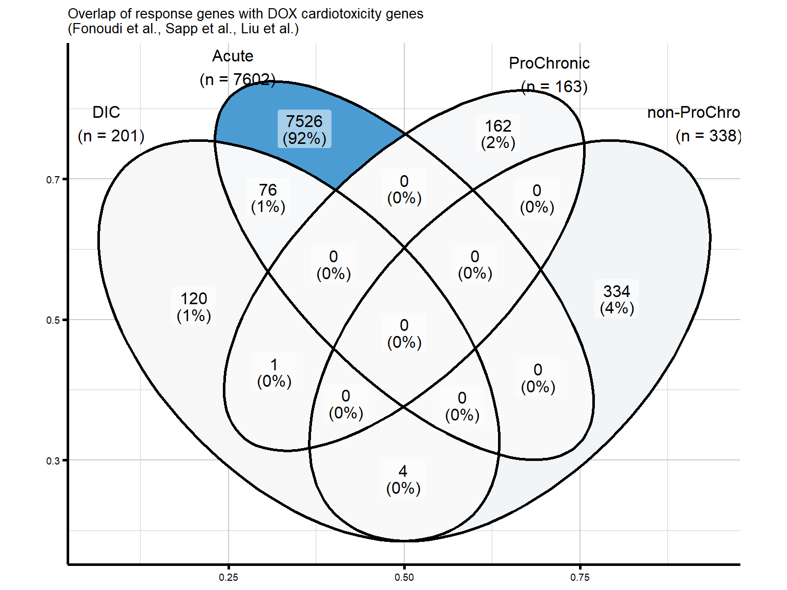
#I am interested in the gene that is overlapping in my ProChronic with the DIC gene set
#POLQ
Figure 7B - Overlapping gene from ProChronic and DIC (POLQ)
#proChronic_gene_list
#DIC_genes

#there are 5 total genes to investigate based on the Venn diagram of overlap with CT genes
#1 overlap with ProChronic
#4 overlap with non-ProChronic

intersect(proChronic_gene_list, DIC_genes)
[1] "10721"proChronic_overlap <- proChronic_gene_list[proChronic_gene_list %in% DIC_genes]
#these give the same results
#10721 Entrez_ID
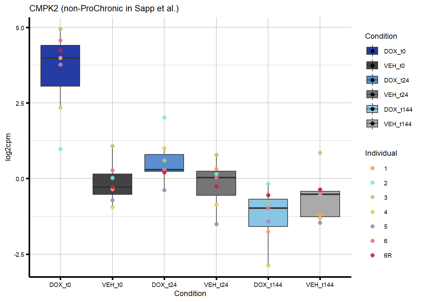
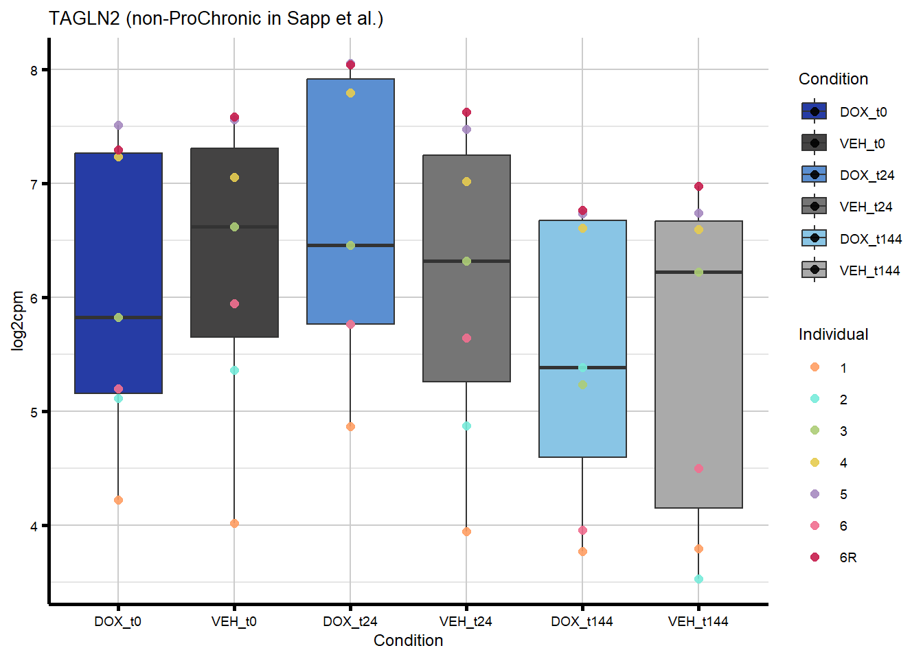
intersect(nonproChronic_gene_list, DIC_genes)[1] "8407" "129607" "30811" "1310" nonproChronic_overlap <- nonproChronic_gene_list[nonproChronic_gene_list %in% DIC_genes]
#these give the same results
#8407, 129607, 30811, 1310 Entrez_ID =
#8407 =
#129607
DIC_cats <- list(
"Fonoudi et al." = fonoudi_ids,
"Liu et al." = liu_ids,
"Sapp et al." = sapp_ids
)
#pull the gene symbol so I can plot log2cpm data
dic_genes_df <- map_dfr(names(DIC_cats), function(cat) {
tibble(
Entrez_ID = intersect(DIC_genes, DIC_cats[[cat]]),
Category = cat
)
})
dim(dic_genes_df)[1] 202 2#202 genes overall from all categories
#filter overlaps for proSus
proChronic_overlap <- dic_genes_df %>%
filter(Entrez_ID %in% proChronic_gene_list)
#1 gene - from Sapp et al
#filter overlaps for recSus
nonproChronic_overlap <- dic_genes_df %>%
filter(Entrez_ID %in% nonproChronic_gene_list)
#4 genes - from Sapp et al
#also sanity check that these genes are DEGs that overlap with proSus recSus
set_for_overlap <- list(
ProChronic = proChronic_overlap$Entrez_ID,
nonproChronic = nonproChronic_overlap$Entrez_ID,
geneSets = unique(unlist(DIC_genes))
)
#read in my factors
#add in colors and factors
txtime_col <- list(
"DOX_t0" = "#263CA5",
"VEH_t0" = "#444343",
"DOX_t24" = "#5B8FD1",
"VEH_t24" = "#757575",
"DOX_t144" = "#89C5E5",
"VEH_t144" = "#AAAAAA"
)
ind_col <- list(
"1" = "#FF9F64",
"2" = "#78EBDA",
"3" = "#ADCD77",
"4" = "#E6CC50",
"5" = "#A68AC0",
"6" = "#F16F90",
"6R" = "#C61E4E"
)
time_col <- list(
"t0" = "#005A4C",
"t24" = "#328477",
"t144" = "#8FB9B1")
tx_col <- list(
"DOX" = "#499FBD",
"VEH" = "#BBBBBC")
#read in my deg_wide dataframe
deg_wide <- readRDS("data/DE/DEGs_overlap_wide_dataframe.RDS")
proChronic_degs <- deg_wide %>%
dplyr::filter(Entrez_ID %in% proChronic_overlap$Entrez_ID)
nonproChronic_degs <- deg_wide %>%
dplyr::filter(Entrez_ID %in% nonproChronic_overlap$Entrez_ID)
#check whether the assumptions are stil the same that the absFC is t0 < t144
#ProChronic
proChronic_pattern <- proChronic_degs %>%
mutate(correct_pattern = absFC_t0 < absFC_t24 & absFC_t24 < absFC_t144)
proChronic_summary <- proChronic_pattern %>%
summarise(
total_genes = n(),
n_correct = sum(correct_pattern, na.rm = TRUE),
percent_correct = 100 * n_correct / total_genes
)
proChronic_summary # A tibble: 1 × 3
total_genes n_correct percent_correct
<int> <int> <dbl>
1 1 1 100#find gene symbols
proChronic_overlap <- proChronic_overlap %>%
mutate(
SYMBOL = mapIds(
org.Hs.eg.db,
keys = Entrez_ID,
column = "SYMBOL",
keytype = "ENTREZID",
multiVals = "first"
)
)
nonproChronic_overlap <- nonproChronic_overlap %>%
mutate(
SYMBOL = mapIds(
org.Hs.eg.db,
keys = Entrez_ID,
column = "SYMBOL",
keytype = "ENTREZID",
multiVals = "first"
)
)
#now plot these example genes for each
boxplot_new <- readRDS("data/DE/boxplot_updated.RDS")
#process the cpm data
process_cpm_data_cormotif <- function(gene_id, expr_df) {
gene_data <- expr_df %>% filter(Entrez_ID == gene_id)
long_data <- gene_data %>%
pivot_longer(
cols = -c(Entrez_ID, SYMBOL),
names_to = "Sample",
values_to = "log2CPM"
) %>%
mutate(
Treatment = case_when(
grepl("DOX", Sample) ~ "DOX",
grepl("VEH", Sample) ~ "VEH",
TRUE ~ NA_character_
),
Timepoint = case_when(
grepl("t0", Sample) ~ "t0",
grepl("t24", Sample) ~ "t24",
grepl("t144", Sample) ~ "t144",
TRUE ~ NA_character_
),
Individual = case_when(
grepl("1$", Sample) ~ "1",
grepl("2$", Sample) ~ "2",
grepl("3$", Sample) ~ "3",
grepl("4$", Sample) ~ "4",
grepl("5$", Sample) ~ "5",
grepl("6$", Sample) ~ "6",
grepl("6R$", Sample) ~ "6R",
TRUE ~ NA_character_
),
Condition = paste(Treatment, Timepoint, sep = "_")
)
# Set factor levels for plotting order
long_data$Condition <- factor(
long_data$Condition,
levels = c("DOX_t0", "VEH_t0",
"DOX_t24", "VEH_t24",
"DOX_t144", "VEH_t144")
)
return(long_data)
}
# Function to generate plots for a set of genes
generate_overlap_plots_cormotif <- function(overlap_df, expr_df, comparison_label) {
plots <- list()
for (gene_id in overlap_df$Entrez_ID) {
gene_data <- process_cpm_data_cormotif(gene_id, expr_df)
# Get SYMBOL and all categories
gene_symbol <- unique(gene_data$SYMBOL)
gene_categories <- overlap_df$Category[overlap_df$Entrez_ID == gene_id]
gene_categories <- paste(unique(gene_categories), collapse = ", ")
p <- ggplot(gene_data, aes(x = Condition,
y = log2CPM,
fill = Condition)) +
geom_boxplot(outlier.shape = NA) +
geom_point(aes(color = Individual), size = 2,
alpha = 0.9,
position = position_identity()) +
scale_fill_manual(values = txtime_col) +
scale_color_manual(values = ind_col) +
ggtitle(paste0(gene_symbol,
" (", comparison_label, " in ", gene_categories, ") ")) +
labs(x = "Condition", y = "log2cpm") +
theme_custom()
#use Entrez_ID + SYMBOL + comparison label for the list name to guarantee uniqueness
plot_name <- paste0(gene_symbol, "_", gene_id, "_", comparison_label)
plots[[plot_name]] <- p
}
return(plots)
}
#generate plots for both (most interested in proChronic overlap with DIC genes)
proChronic_plots <- generate_overlap_plots_cormotif(proChronic_overlap,
boxplot_new, "ProChronic")
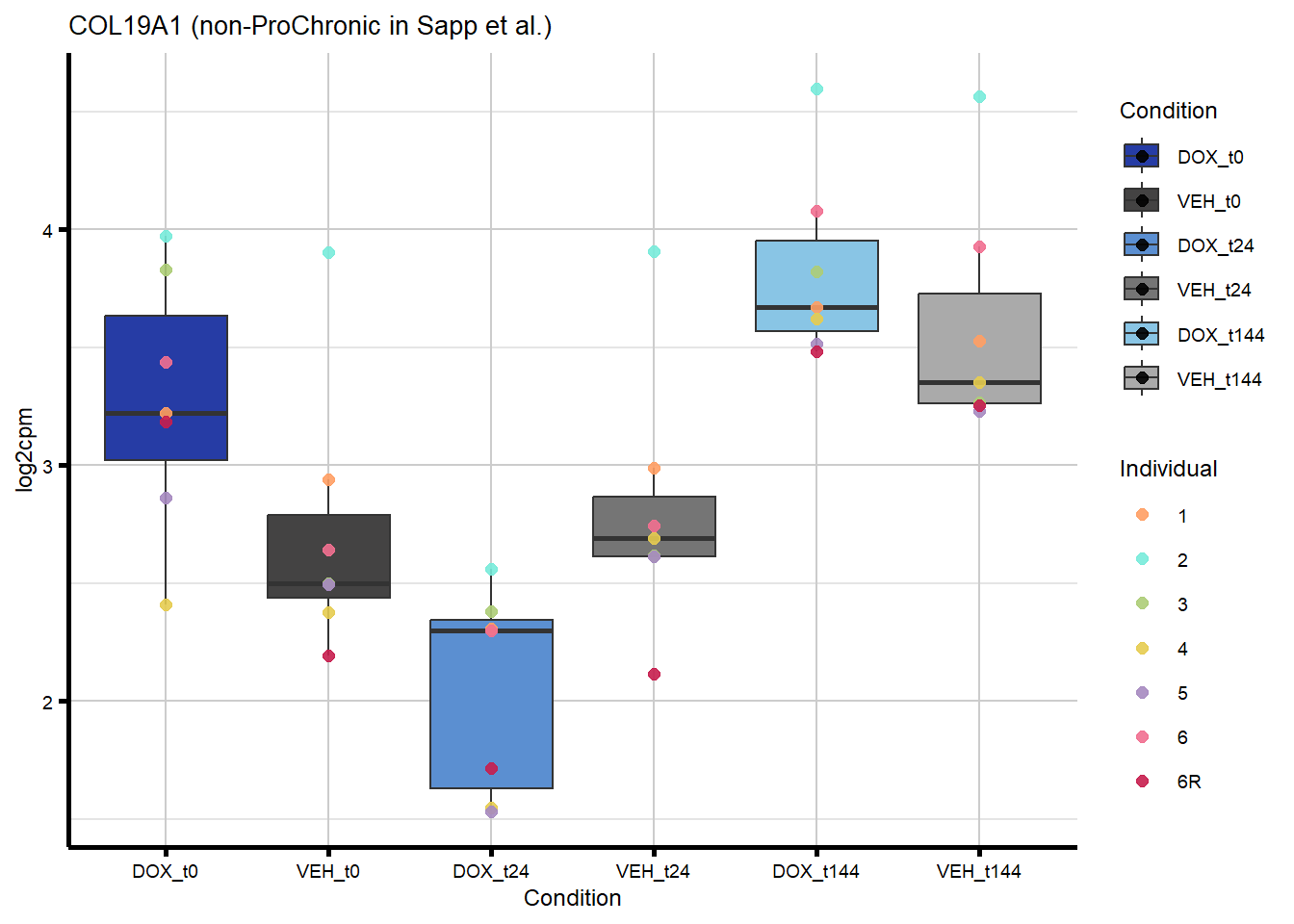
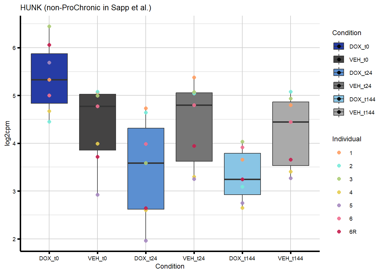
nonproChronic_plots <- generate_overlap_plots_cormotif(nonproChronic_overlap,
boxplot_new, "non-ProChronic")
#preview all plots
for (p in c(proChronic_plots, nonproChronic_plots)) print(p)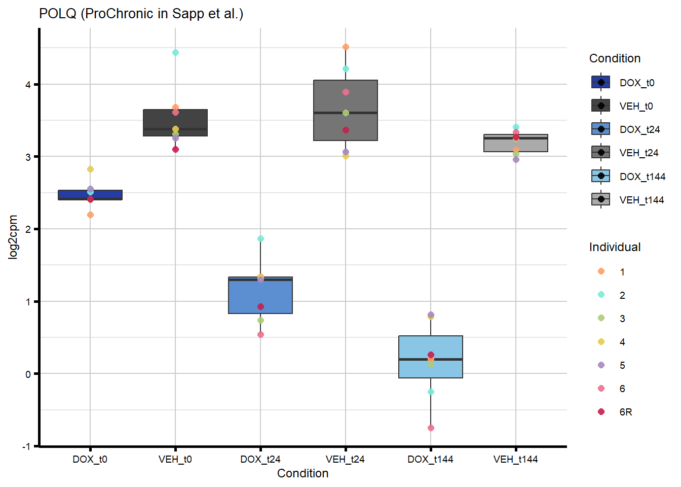
#save all of these plots with unique names
# for (plot_name in names(proSus_plots)) {
#   save_plot(proSus_plots[[plot_name]],
#             filename = paste0("ExGene_proSus_", plot_name, "_EMP"),
#             folder = output_folder)
# }
#
# for (plot_name in names(notproSus_plots)) {
#   save_plot(notproSus_plots[[plot_name]],
#             filename = paste0("ExGene_notproSus_", plot_name, "_EMP"),
#             folder = output_folder)
# }


#POLQ is the gene that is overlapping between DIC and ProChronic
Figure 7C - Overlap of response genes with heart failure risk genes
We pulled the associations for heart failure (HF) from the GWAS catalogue for this analysis.
#read in the HF GWAS gene set from the GWAS catalog

hf_gwas_genes <- readRDS("data/Fig7/HF_gwas_genelist.RDS")
hf_gwas_genes_list <- hf_gwas_genes$Entrez_ID

venn_proChronic_list_HF <- list(
  HF = as.character(hf_gwas_genes_list),
  Acute = as.character(final_genes_1_RUV),
  ProChronic = as.character(proChronic_gene_list),
  nonProChronic = as.character(nonproChronic_gene_list)
)

venn_proChronic_HF <- ggVennDiagram(
  venn_proChronic_list_HF,
  category.names = c("HF GWAS\n (n = 299)",
                     "Acute \n (n = 7602)",
                     "ProChronic \n (n = 163)",
                     "non-ProChronic \n (n = 338)")
) +
  ggtitle("Overlap of response genes with heart failure risk genes \n(Cerezo et al.)") +
  labs(x = NULL, y = NULL) +
  scale_fill_gradient(low = "#F9F9F9", high = "#4B9CD3") +
  theme_custom() +
  theme(legend.position = "none")


print(venn_proChronic_HF)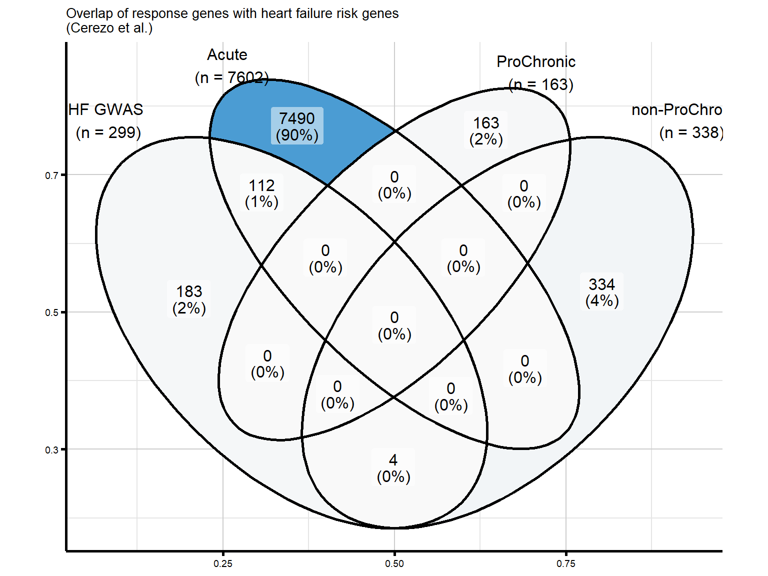
# save_plot(
# plot = venn_proSus_HF,
# filename = "Venn_HF_proSus_EMP",
# folder = output_folder,
# height = 6,
# width = 8
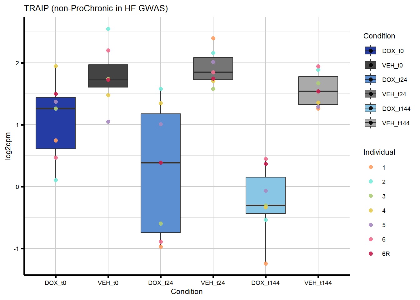
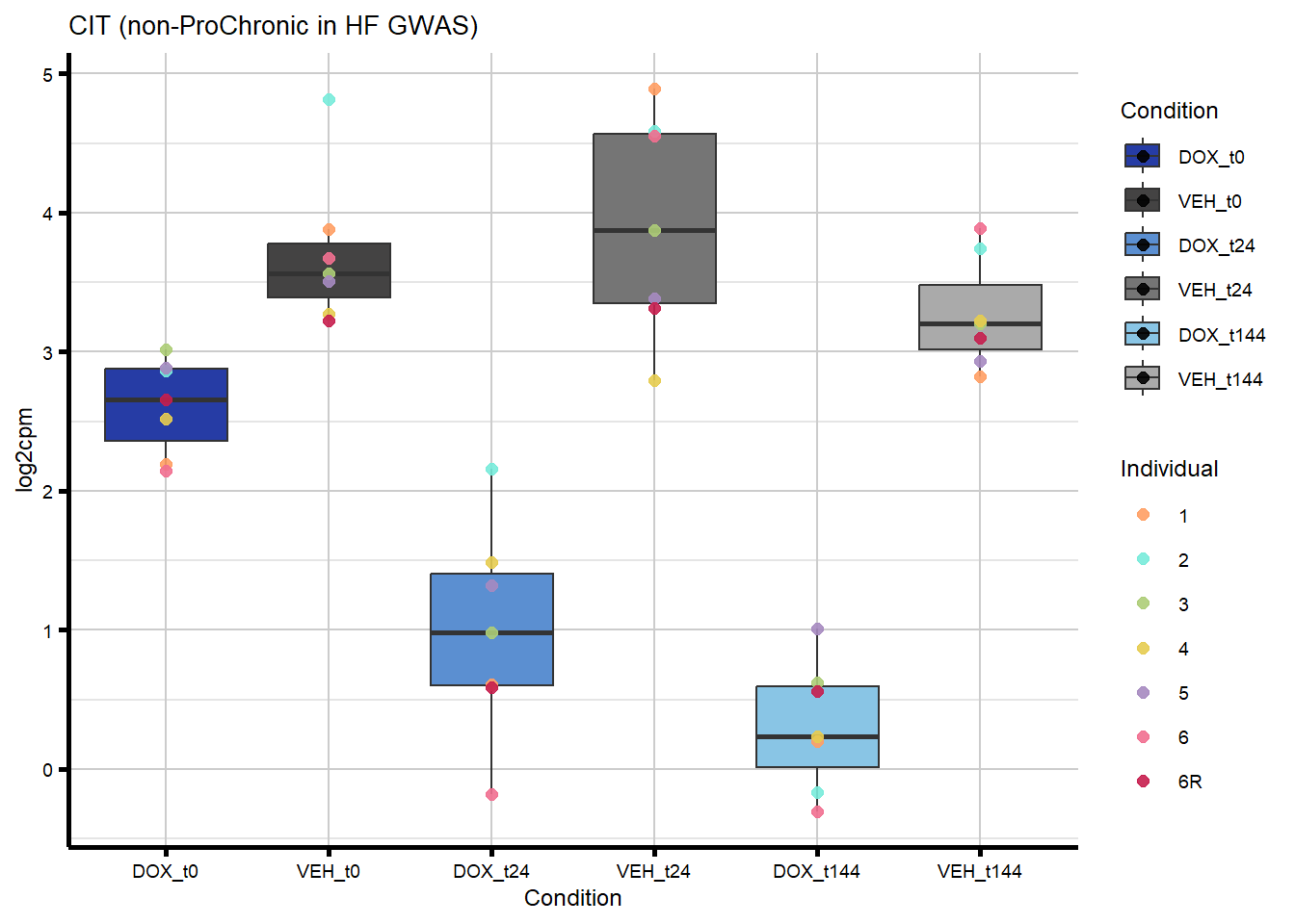
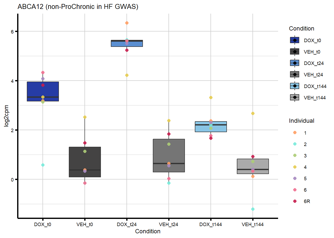
# )Figure 7D - Overlap of HF risk genes with non-ProChronic (TIRAP)
#there are 4 total genes to investigate based on the Venn diagram of overlap with HF GWAS Genes
#4 overlap with non-ProChronic

nonproChronic_overlap <- nonproChronic_gene_list[nonproChronic_gene_list %in% hf_gwas_genes_list]
#Entrez_IDs - 11113, 26154, 10293, 1026

HF_cats <- list(
  "HF GWAS" = hf_gwas_genes_list
)

hf_gwas_cats <- list(
  "HF GWAS Genes" = unique(na.omit(hf_gwas_genes_list))
)

#pull the gene symbol so I can plot log2cpm data
hf_genes_df <- map_dfr(names(HF_cats), function(cat) {
  tibble(
    Entrez_ID = intersect(hf_gwas_genes_list, HF_cats[[cat]]),
    Category = cat
  )
})

dim(hf_genes_df)
[1] 299 2#filter overlaps for notproSus
nonproChronic_overlap_hf <- hf_genes_df %>%
filter(Entrez_ID %in% nonproChronic_gene_list)
#4 genes
#read in my dataframe for plotting log2cpm genes
deg_wide <- readRDS("data/DE/DEGs_overlap_wide_dataframe.RDS")
nonproChronic_degs <- deg_wide %>%
dplyr::filter(Entrez_ID %in% nonproChronic_overlap_hf$Entrez_ID)
#check whether the assumptions are stil the same that the absFC is t0 < t144
#find gene symbols
nonproChronic_overlap_hf <- nonproChronic_overlap_hf %>%
mutate(
SYMBOL = mapIds(
org.Hs.eg.db,
keys = Entrez_ID,
column = "SYMBOL",
keytype = "ENTREZID",
multiVals = "first"
)
)
#now plot these example genes for each
boxplot_new <- readRDS("data/DE/boxplot_updated.RDS")
#process the cpm data
process_cpm_data_cormotif <- function(gene_id, expr_df) {
gene_data <- expr_df %>% filter(Entrez_ID == gene_id)
long_data <- gene_data %>%
pivot_longer(
cols = -c(Entrez_ID, SYMBOL),
names_to = "Sample",
values_to = "log2CPM"
) %>%
mutate(
Treatment = case_when(
grepl("DOX", Sample) ~ "DOX",
grepl("VEH", Sample) ~ "VEH",
TRUE ~ NA_character_
),
Timepoint = case_when(
grepl("t0", Sample) ~ "t0",
grepl("t24", Sample) ~ "t24",
grepl("t144", Sample) ~ "t144",
TRUE ~ NA_character_
),
Individual = case_when(
grepl("1$", Sample) ~ "1",
grepl("2$", Sample) ~ "2",
grepl("3$", Sample) ~ "3",
grepl("4$", Sample) ~ "4",
grepl("5$", Sample) ~ "5",
grepl("6$", Sample) ~ "6",
grepl("6R$", Sample) ~ "6R",
TRUE ~ NA_character_
),
Condition = paste(Treatment, Timepoint, sep = "_")
)
#set factor levels for plotting order
long_data$Condition <- factor(
long_data$Condition,
levels = c("DOX_t0", "VEH_t0",
"DOX_t24", "VEH_t24",
"DOX_t144", "VEH_t144")
)
return(long_data)
}
#function to generate plots for a set of genes
generate_overlap_plots_cormotif <- function(overlap_df, expr_df, comparison_label) {
plots <- list()
for (gene_id in overlap_df$Entrez_ID) {
gene_data <- process_cpm_data_cormotif(gene_id, expr_df)
# Get SYMBOL and all categories
gene_symbol <- unique(gene_data$SYMBOL)
gene_categories <- overlap_df$Category[overlap_df$Entrez_ID == gene_id]
gene_categories <- paste(unique(gene_categories), collapse = ", ")
p <- ggplot(gene_data, aes(x = Condition,
y = log2CPM,
fill = Condition)) +
geom_boxplot(outlier.shape = NA) +
geom_point(aes(color = Individual), size = 2,
alpha = 0.9,
position = position_identity()) +
scale_fill_manual(values = txtime_col) +
scale_color_manual(values = ind_col) +
ggtitle(paste0(gene_symbol,
" (", comparison_label, " in ", gene_categories, ") ")) +
labs(x = "Condition", y = "log2cpm") +
theme_custom()
#use Entrez_ID + SYMBOL + comparison label for the list name to guarantee uniqueness
plot_name <- paste0(gene_symbol, "_", gene_id, "_", comparison_label)
plots[[plot_name]] <- p
}
return(plots)
}
#generate plots for notproSus overlap genes
nonproChronic_plots_hf <- generate_overlap_plots_cormotif(nonproChronic_overlap_hf,
boxplot_new, "non-ProChronic")
#preview all plots
for (p in c(nonproChronic_plots_hf)) print(p)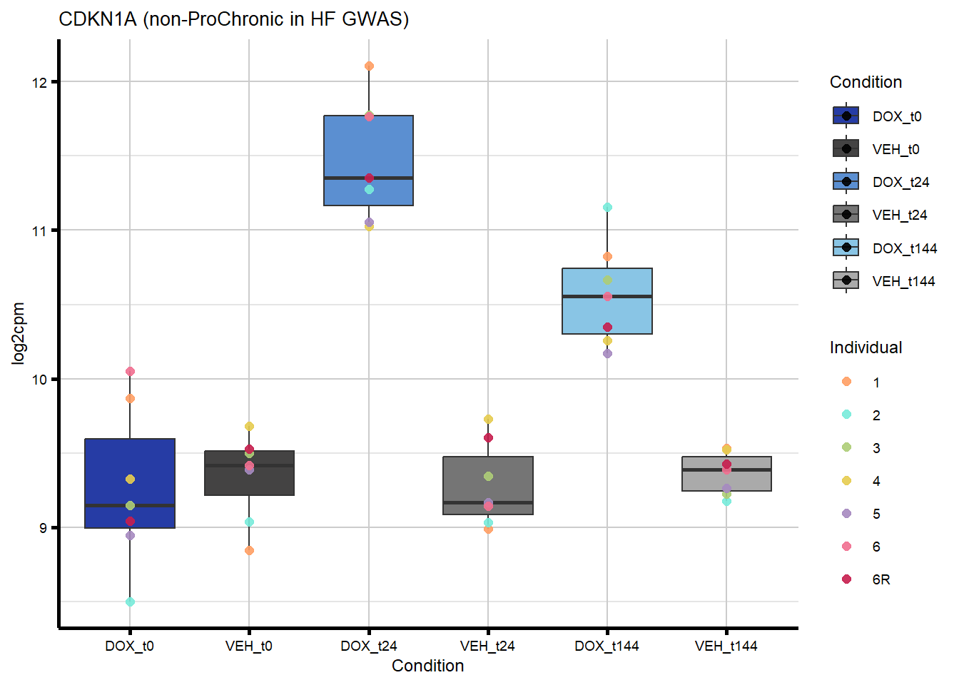
#save all of these plots with unique names
# for (plot_name in names(nonproChronic_plots_hf)) {
#   save_plot(nonproChronic_plots_hf[[plot_name]],
#             filename = paste0("ExGene_HF_nonproChronic_", plot_name, "_EMP"),
#             folder = output_folder)
# }

#I plotted TIRAP as an example of a gene that overlaps with non-proChronic in the HF GWAS set
sessionInfo()R version 4.4.2 (2024-10-31 ucrt)
Platform: x86_64-w64-mingw32/x64
Running under: Windows 11 x64 (build 22000)
Matrix products: default
locale:
[1] LC_COLLATE=English_United States.utf8
[2] LC_CTYPE=English_United States.utf8
[3] LC_MONETARY=English_United States.utf8
[4] LC_NUMERIC=C
[5] LC_TIME=English_United States.utf8
time zone: America/Chicago
tzcode source: internal
attached base packages:
[1] stats4 grid stats graphics grDevices utils datasets
[8] methods base
other attached packages:
[1] eulerr_7.0.2 ggVennDiagram_1.5.2 gprofiler2_0.2.3
[4] org.Hs.eg.db_3.20.0 AnnotationDbi_1.68.0 IRanges_2.40.0
[7] S4Vectors_0.44.0 Biobase_2.66.0 BiocGenerics_0.52.0
[10] circlize_0.4.16 reshape2_1.4.4 readxl_1.4.5
[13] lubridate_1.9.4 forcats_1.0.0 stringr_1.5.1
[16] dplyr_1.1.4 purrr_1.0.4 readr_2.1.5
[19] tidyr_1.3.1 tibble_3.2.1 ggplot2_3.5.2
[22] tidyverse_2.0.0 workflowr_1.7.1
loaded via a namespace (and not attached):
[1] tidyselect_1.2.1 viridisLite_0.4.2 farver_2.1.2
[4] blob_1.2.4 Biostrings_2.74.0 lazyeval_0.2.2
[7] fastmap_1.2.0 promises_1.3.2 digest_0.6.37
[10] timechange_0.3.0 lifecycle_1.0.4 processx_3.8.6
[13] KEGGREST_1.46.0 RSQLite_2.3.9 magrittr_2.0.3
[16] compiler_4.4.2 rlang_1.1.6 sass_0.4.10
[19] tools_4.4.2 yaml_2.3.10 data.table_1.17.0
[22] knitr_1.50 labeling_0.4.3 htmlwidgets_1.6.4
[25] bit_4.5.0 plyr_1.8.9 RColorBrewer_1.1-3
[28] withr_3.0.2 git2r_0.36.2 colorspace_2.1-1
[31] scales_1.4.0 cli_3.6.3 rmarkdown_2.29
[34] crayon_1.5.3 generics_0.1.4 rstudioapi_0.17.1
[37] httr_1.4.7 tzdb_0.5.0 DBI_1.2.3
[40] cachem_1.1.0 zlibbioc_1.52.0 cellranger_1.1.0
[43] XVector_0.46.0 vctrs_0.6.5 jsonlite_2.0.0
[46] callr_3.7.6 hms_1.1.3 bit64_4.5.2
[49] plotly_4.10.4 jquerylib_0.1.4 glue_1.8.0
[52] ps_1.9.1 stringi_1.8.7 shape_1.4.6.1
[55] gtable_0.3.6 later_1.4.2 GenomeInfoDb_1.42.3
[58] UCSC.utils_1.2.0 pillar_1.10.2 htmltools_0.5.8.1
[61] GenomeInfoDbData_1.2.13 R6_2.6.1 rprojroot_2.0.4
[64] evaluate_1.0.3 png_0.1-8 memoise_2.0.1
[67] httpuv_1.6.16 bslib_0.9.0 Rcpp_1.0.14
[70] whisker_0.4.1 xfun_0.52 fs_1.6.6
[73] getPass_0.2-4 pkgconfig_2.0.3 GlobalOptions_0.1.2