DE
Emma M Pfortmiller
Last updated: 2026-01-13
Checks: 6 1
Knit directory: Dissrt/
This reproducible R Markdown analysis was created with workflowr (version 1.7.1). The Checks tab describes the reproducibility checks that were applied when the results were created. The Past versions tab lists the development history.
The R Markdown file has staged changes. To know which version of the
R Markdown file created these results, you’ll want to first commit it to
the Git repo. If you’re still working on the analysis, you can ignore
this warning. When you’re finished, you can run
wflow_publish to commit the R Markdown file and build the
HTML.
Great job! The global environment was empty. Objects defined in the global environment can affect the analysis in your R Markdown file in unknown ways. For reproduciblity it’s best to always run the code in an empty environment.
The command set.seed(20250926) was run prior to running
the code in the R Markdown file. Setting a seed ensures that any results
that rely on randomness, e.g. subsampling or permutations, are
reproducible.
Great job! Recording the operating system, R version, and package versions is critical for reproducibility.
Nice! There were no cached chunks for this analysis, so you can be confident that you successfully produced the results during this run.
Great job! Using relative paths to the files within your workflowr project makes it easier to run your code on other machines.
Great! You are using Git for version control. Tracking code development and connecting the code version to the results is critical for reproducibility.
The results in this page were generated with repository version b9f416f. See the Past versions tab to see a history of the changes made to the R Markdown and HTML files.
Note that you need to be careful to ensure that all relevant files for
the analysis have been committed to Git prior to generating the results
(you can use wflow_publish or
wflow_git_commit). workflowr only checks the R Markdown
file, but you know if there are other scripts or data files that it
depends on. Below is the status of the Git repository when the results
were generated:
Ignored files:
    Ignored:    .Rhistory
    Ignored:    .Rproj.user/
    Ignored:    data/cmf/
    Ignored:    data/counts/
    Ignored:    data/de/
    Ignored:    data/genesets/
    Ignored:    data/theme/

Staged changes:
    Modified1:  DE.Rmd
    Modified2:  analysis/DE.Rmd
    Modified:   analysis/QC_Subset.Rmd
Note that any generated files, e.g. HTML, png, CSS, etc., are not included in this status report because it is ok for generated content to have uncommitted changes.
There are no past versions. Publish this analysis with
wflow_publish() to start tracking its development.
#Load Libraries
#Define plot theme
# Define the custom theme
# plot_theme_custom <- function() {
#   theme_minimal() +
#     theme(
#       #line for x and y axis
#       axis.line = element_line(linewidth = 1,
#                                color = "black"),
#
#       #axis ticks only on x and y, length standard
#       axis.ticks.x = element_line(color = "black",
#                                 linewidth = 1),
#       axis.ticks.y = element_line(color = "black",
#                                 linewidth = 1),
#       axis.ticks.length = unit(0.05, "in"),
#
#       #text and font
#       axis.text = element_text(color = "black",
#                                family = "Arial",
#                                size = 8),
#       axis.title = element_text(color = "black",
#                                 family = "Arial",
#                                 size = 10),
#       legend.text = element_text(color = "black",
#                                  family = "Arial",
#                                  size = 8),
#       legend.title = element_text(color = "black",
#                                   family = "Arial",
#                                   size = 10),
#       plot.title = element_text(color = "black",
#                                 family = "Arial",
#                                 size = 12),
#
#       #blank background and border
#       panel.background = element_blank(),
#       panel.border = element_blank(),
#
#       #gridlines for alignment
#       panel.grid.major = element_line(color = "grey80", linewidth = 0.5),  #grey major grid for align in illus
#       panel.grid.minor = element_line(color = "grey90", linewidth = 0.5) #grey minor grid for align in illus
#     )
# }

# saveRDS(plot_theme_custom, "data/plot_theme_custom.RDS")

theme_custom <- readRDS("data/plot_theme_custom.RDS")
#Define saving plots as pdfs
save_plot <- function(plot, filename,
                      folder = ".",
                      width = 8,
                      height = 6,
                      units = "in",
                      dpi = 300,
                      add_date = TRUE) {
  if (missing(filename)) stop("Please provide a filename (without extension) for the plot.")

  date_str <- if (add_date) paste0("_", format(Sys.Date(), "%y%m%d")) else ""
  pdf_file <- file.path(folder, paste0(filename, date_str, ".pdf"))
  png_file <- file.path(folder, paste0(filename, date_str, ".png"))
  ggsave(filename = pdf_file, plot = plot, device = cairo_pdf, width = width, height = height, units = units, bg = "transparent")
  ggsave(filename = png_file, plot = plot, device = "png", width = width, height = height, units = units, dpi = dpi, bg = "transparent")
  message("Saved plot as Cairo PDF: ", pdf_file)
  message("Saved plot as PNG: ", png_file)
}

output_folder <- "C:/Users/emmap/OneDrive/Desktop/Ward Lab/Experiments/Stressor Project/Full Set RNAseq/plots"


#save plot function created
#to use: just define the plot name, filename_base, width, height
#Factors and Colors
#each of these to be used after pairwise comparison save individual

####STIMULI####
# stim_list <- list(
#   "Tunicamycin" = "TUN",
#   "Thapsigargin" = "THA",
#   "Doxorubicin" = "DOX",
#   "Nutlin-3" = "NUTL",
#   "Lipopolysaccharides" = "LPS",
#   "Tumor Necrosis Factor alpha" = "TNFa",
#   "Bisphenol A" = "BPA",
#   "Perfluorooctanoic Acid" = "PFOA"
# )
# stimuli_vec <- unlist(lapply(names(stim_list), function(cat) {
#   setNames(rep(cat, length(stim_list[[cat]])), stim_list[[cat]])
# }))
# saveRDS(stimuli_vec, "data/theme/stimuli_fullname_vector.RDS")
stim_vec <- readRDS("data/theme/stimuli_fullname_vector.RDS")

####RESPONSE CATEGORY####
# resp_list <- list(
#   UPR = c("TUN", "THA"),
#   DDR = c("DOX", "NUTL"),
#   IMR = c("LPS", "TNFa"),
#   MMR = c("BPA", "PFOA")
# )
# response_vec <- unlist(lapply(names(resp_list), function(cat) {
#   setNames(rep(cat, length(resp_list[[cat]])), resp_list[[cat]])
# }))
# saveRDS(response_vec, "data/theme/response_categories_vector.RDS")
response_vec <- readRDS("data/theme/response_categories_vector.RDS")

####SPECIES####
# spec_list <- list(
#   Human = "H",
#   Chimp = "C"
# )
# species_vec <- unlist(lapply(names(spec_list), function(cat) {
#   setNames(rep(cat, length(spec_list[[cat]])), spec_list[[cat]])
# }))
# saveRDS(species_vec, "data/theme/species_vector.RDS")
species_vec <- readRDS("data/theme/species_vector.RDS")

####TIME####
# time_list <- list(
#   "2hr" = "2",
#   "24hr" = "24"
# )
# time_vec <- unlist(lapply(names(time_list), function(cat) {
#   setNames(rep(cat, length(time_list[[cat]])), time_list[[cat]])
# }))
# saveRDS(time_vec, "data/theme/time_vector.RDS")
time_vec <- readRDS("data/theme/time_vector.RDS")

####INDIVIDUAL####
# ind_list <- list(
#   H24280 = "H1",
#   H28126 = "H2",
#   "84-1" = "H3",
#   H21792 = "H4",
#   H20682 = "H5",
#   H22422 = "H6",
#   "78-1" = "H7",
#   C3647 = "C1",
#   C8861 = "C2",
#   C4020 = "C3",
#   C3649 = "C4",
#   C3651 = "C5",
#   C40280 = "C6",
#   C4955 = "C7"
# )
# ind_vec <- unlist(lapply(names(ind_list), function (cat) {
#   setNames(rep(cat, length(ind_list[[cat]])), ind_list[[cat]])
# }))
# saveRDS(ind_vec, "data/theme/individual_vector.RDS")
ind_vec <- readRDS("data/theme/individual_vector.RDS")
Read in Dataframes
#read in my counts file for my subset of samples
hc_counts_sub <- readRDS("data/counts/hc_counts_subset_entrez.RDS")

#read in my cpm matrix (already subset)
hc_cpm_matrix <- readRDS("data/counts/hc_cpm_filtered_matrix_subset.RDS")

#read in my metadata for this subset
metadata_sub <- read_csv("data/counts/metadata_subset.csv")
Differential Expression Analysis
#filter my raw counts (subset of samples) to remove lowly expressed genes as above

x <- hc_counts_sub[row.names(hc_cpm_matrix),]
# dim(x)

# saveRDS(x, "data/de/x_dge_counts_allind_subset.RDS")

x <- readRDS("data/de/x_dge_counts_allind_subset.RDS")

#use metadata_sub to match
meta_de <- metadata_sub

#ensure that the names are matched up properly
identical(meta_de$Final_sample_name, colnames(x))
[1] TRUEcolnames(x) <- meta_de$Final_sample_name
rownames(meta_de) <- meta_de$Final_sample_name
meta_de$Cond <- make.names(meta_de$Cond)
meta_de$Ind <- as.character(meta_de$Ind)
# saveRDS(meta_de, "data/de/metadata_2_de.RDS")
# saveRDS(x, "data/de/x_counts_de.RDS")
#create my DGElist object
dge <- DGEList(counts = x)
dge$samples$group <- factor(meta_de$Cond)
dge <- calcNormFactors(dge, method = "TMM")
# saveRDS(dge, "data/de/dge_matrix.RDS")
#check the normalization factors from TMM normalization of the libraries
dge$samples group lib.size norm.factors
TUN_2_C1 TUN_2_C 4959120 0.8274652
THA_2_C1 THA_2_C 7407002 0.8388147
DMSO_2_C1 DMSO_2_C 6447319 0.8277064
TUN_24_C1 TUN_24_C 5920073 0.8223902
THA_24_C1 THA_24_C 5605707 0.9282232
DOX_24_C1 DOX_24_C 4915306 0.6852739
NUTL_24_C1 NUTL_24_C 5968030 0.8527996
DMSO_24_C1 DMSO_24_C 4163362 0.8510154
LPS_24_C1 LPS_24_C 5540367 0.8262713
TNFa_24_C1 TNFa_24_C 5461910 0.8500622
H2O_24_C1 H2O_24_C 6343704 0.8316516
BPA_24_C1 BPA_24_C 5806762 0.7918941
PFOA_24_C1 PFOA_24_C 5763792 0.8332842
EtOH_24_C1 EtOH_24_C 5329162 0.8255942
TUN_2_C2 TUN_2_C 3669613 0.9760496
THA_2_C2 THA_2_C 3835409 1.0457465
DMSO_2_C2 DMSO_2_C 4098895 0.9925365
TUN_24_C2 TUN_24_C 3915885 1.0341810
THA_24_C2 THA_24_C 3723396 0.9797107
DOX_24_C2 DOX_24_C 3475457 1.1264528
NUTL_24_C2 NUTL_24_C 3510587 0.9951095
DMSO_24_C2 DMSO_24_C 3818926 0.9726100
LPS_24_C2 LPS_24_C 4140244 0.9601131
TNFa_24_C2 TNFa_24_C 3740690 0.9837099
H2O_24_C2 H2O_24_C 3890138 0.9538141
BPA_24_C2 BPA_24_C 3939470 0.9598972
PFOA_24_C2 PFOA_24_C 4189725 0.9652969
EtOH_24_C2 EtOH_24_C 3571535 0.9800994
TUN_2_C3 TUN_2_C 4010528 1.0143085
THA_2_C3 THA_2_C 4087377 1.0867888
DMSO_2_C3 DMSO_2_C 3331058 1.0281897
TUN_24_C3 TUN_24_C 3772938 1.0495732
THA_24_C3 THA_24_C 3628245 1.0557194
DOX_24_C3 DOX_24_C 2749174 1.1421786
NUTL_24_C3 NUTL_24_C 3817234 1.0822000
DMSO_24_C3 DMSO_24_C 5146135 1.0798687
LPS_24_C3 LPS_24_C 3371202 1.0302273
TNFa_24_C3 TNFa_24_C 3768725 1.0513896
H2O_24_C3 H2O_24_C 3045735 1.0425282
BPA_24_C3 BPA_24_C 4024472 1.0525834
PFOA_24_C3 PFOA_24_C 4158259 1.0401244
EtOH_24_C3 EtOH_24_C 3078091 1.0443458
TUN_2_C4 TUN_2_C 5442200 1.0258397
THA_2_C4 THA_2_C 4842067 1.0941637
DMSO_2_C4 DMSO_2_C 8294030 1.0507750
TUN_24_C4 TUN_24_C 6084143 1.0723319
THA_24_C4 THA_24_C 4752713 1.0542360
DOX_24_C4 DOX_24_C 5587235 1.2378495
NUTL_24_C4 NUTL_24_C 5424888 1.0433478
DMSO_24_C4 DMSO_24_C 4936901 1.0322069
LPS_24_C4 LPS_24_C 5044954 1.0239242
TNFa_24_C4 TNFa_24_C 5449243 1.0173841
H2O_24_C4 H2O_24_C 6114673 1.0155054
BPA_24_C4 BPA_24_C 5448746 1.0284361
PFOA_24_C4 PFOA_24_C 5170408 1.0337958
EtOH_24_C4 EtOH_24_C 4687966 1.0416165
TUN_2_C5 TUN_2_C 5260281 0.8959149
DMSO_2_C5 DMSO_2_C 4980521 0.9150542
TUN_24_C5 TUN_24_C 2422629 0.9663321
THA_24_C5 THA_24_C 5220437 0.9338753
DOX_24_C5 DOX_24_C 3857127 0.9379252
NUTL_24_C5 NUTL_24_C 5431835 0.9607412
DMSO_24_C5 DMSO_24_C 6072407 0.9439351
LPS_24_C5 LPS_24_C 4927576 0.9359844
TNFa_24_C5 TNFa_24_C 3324595 0.9542558
H2O_24_C5 H2O_24_C 3415761 0.9319109
BPA_24_C5 BPA_24_C 4828093 0.9989147
PFOA_24_C5 PFOA_24_C 2729739 0.9668128
EtOH_24_C5 EtOH_24_C 4543163 0.9876224
TUN_2_C6 TUN_2_C 4132658 0.9435674
THA_2_C6 THA_2_C 5287746 1.0344496
DMSO_2_C6 DMSO_2_C 4281498 0.9484976
TUN_24_C6 TUN_24_C 4642733 1.0033246
THA_24_C6 THA_24_C 3658060 0.9831190
DOX_24_C6 DOX_24_C 3544684 0.9549855
NUTL_24_C6 NUTL_24_C 4481917 0.9811213
DMSO_24_C6 DMSO_24_C 2687838 0.9945722
LPS_24_C6 LPS_24_C 3299381 1.0397990
TNFa_24_C6 TNFa_24_C 4596178 0.9443678
H2O_24_C6 H2O_24_C 5662044 0.9662587
BPA_24_C6 BPA_24_C 4081570 1.0223036
PFOA_24_C6 PFOA_24_C 4478352 0.9924562
EtOH_24_C6 EtOH_24_C 4526909 0.9963390
TUN_2_C7 TUN_2_C 4021553 1.0734842
THA_2_C7 THA_2_C 3638538 1.0967124
DMSO_2_C7 DMSO_2_C 4396029 1.0775258
TUN_24_C7 TUN_24_C 4867408 1.1030082
THA_24_C7 THA_24_C 4874929 1.0320511
DOX_24_C7 DOX_24_C 10856556 1.0930037
NUTL_24_C7 NUTL_24_C 4774607 1.0827795
DMSO_24_C7 DMSO_24_C 5061193 1.0998111
LPS_24_C7 LPS_24_C 4713485 1.0527685
TNFa_24_C7 TNFa_24_C 5033060 1.0676786
H2O_24_C7 H2O_24_C 4909794 1.0786616
BPA_24_C7 BPA_24_C 5500744 1.0744277
PFOA_24_C7 PFOA_24_C 4973477 1.0795022
EtOH_24_C7 EtOH_24_C 5864356 1.0900827
TUN_2_H1 TUN_2_H 3927492 1.0407090
THA_2_H1 THA_2_H 4477304 1.1737657
DMSO_2_H1 DMSO_2_H 5131738 1.1621535
TUN_24_H1 TUN_24_H 5063593 1.1343096
THA_24_H1 THA_24_H 4161183 1.0143056
DOX_24_H1 DOX_24_H 3830291 1.2342547
NUTL_24_H1 NUTL_24_H 4109224 1.1999306
DMSO_24_H1 DMSO_24_H 4884450 1.1491010
LPS_24_H1 LPS_24_H 4714234 1.1306675
TNFa_24_H1 TNFa_24_H 3652733 1.0618520
H2O_24_H1 H2O_24_H 5644094 1.0461864
BPA_24_H1 BPA_24_H 4939444 1.0836678
PFOA_24_H1 PFOA_24_H 3516211 1.0987721
EtOH_24_H1 EtOH_24_H 5021963 1.1554326
TUN_2_H2 TUN_2_H 4084086 0.9746956
THA_2_H2 THA_2_H 4334715 1.0004025
DMSO_2_H2 DMSO_2_H 3795254 0.9936030
TUN_24_H2 TUN_24_H 2368177 0.9993921
THA_24_H2 THA_24_H 3755675 0.9624449
DOX_24_H2 DOX_24_H 3675934 1.1199444
NUTL_24_H2 NUTL_24_H 5622940 1.0014470
DMSO_24_H2 DMSO_24_H 4466963 0.9902182
LPS_24_H2 LPS_24_H 3953259 0.9789006
TNFa_24_H2 TNFa_24_H 4558984 0.9482547
H2O_24_H2 H2O_24_H 4393881 0.9845595
BPA_24_H2 BPA_24_H 4262074 0.9724784
PFOA_24_H2 PFOA_24_H 4637013 0.9889370
EtOH_24_H2 EtOH_24_H 4045494 0.9847932
TUN_2_H3 TUN_2_H 4624289 0.9107778
THA_2_H3 THA_2_H 4671793 0.9845150
DMSO_2_H3 DMSO_2_H 4456642 0.9192210
TUN_24_H3 TUN_24_H 829325 0.9539374
THA_24_H3 THA_24_H 4447384 0.9255098
DOX_24_H3 DOX_24_H 3517136 0.8333112
NUTL_24_H3 NUTL_24_H 4836535 0.9288940
DMSO_24_H3 DMSO_24_H 4938430 0.9359783
LPS_24_H3 LPS_24_H 5750646 0.9256010
TNFa_24_H3 TNFa_24_H 7009774 0.8982110
H2O_24_H3 H2O_24_H 9615797 0.9267303
BPA_24_H3 BPA_24_H 3949790 0.9569316
PFOA_24_H3 PFOA_24_H 158890 1.0312532
EtOH_24_H3 EtOH_24_H 4850466 0.9208235
TUN_2_H4 TUN_2_H 4736981 0.9654103
THA_2_H4 THA_2_H 5126455 0.9837877
DMSO_2_H4 DMSO_2_H 5532136 0.9503962
TUN_24_H4 TUN_24_H 5531052 0.9419443
THA_24_H4 THA_24_H 5640304 0.9726737
DOX_24_H4 DOX_24_H 5837993 0.9887585
NUTL_24_H4 NUTL_24_H 4600568 0.9673994
DMSO_24_H4 DMSO_24_H 3931849 0.9670037
LPS_24_H4 LPS_24_H 3368315 0.9658248
TNFa_24_H4 TNFa_24_H 4620515 0.9353418
H2O_24_H4 H2O_24_H 5519677 0.9636465
BPA_24_H4 BPA_24_H 4790327 0.9270243
PFOA_24_H4 PFOA_24_H 6228314 0.9400187
EtOH_24_H4 EtOH_24_H 5056429 0.9731401
TUN_2_H5 TUN_2_H 3821591 1.0196187
THA_2_H5 THA_2_H 3945095 0.9736086
DMSO_2_H5 DMSO_2_H 2953839 0.9584474
TUN_24_H5 TUN_24_H 3983888 1.0275336
THA_24_H5 THA_24_H 1500011 1.0331216
DOX_24_H5 DOX_24_H 4181520 1.0726851
NUTL_24_H5 NUTL_24_H 3669772 1.0558622
DMSO_24_H5 DMSO_24_H 4899358 1.0161433
LPS_24_H5 LPS_24_H 4353197 0.9836018
TNFa_24_H5 TNFa_24_H 4229938 1.0121347
H2O_24_H5 H2O_24_H 4933369 1.0209506
BPA_24_H5 BPA_24_H 4807144 1.0173453
PFOA_24_H5 PFOA_24_H 4168658 0.9920302
EtOH_24_H5 EtOH_24_H 3892381 0.9857585
TUN_2_H6 TUN_2_H 4525698 0.9885124
THA_2_H6 THA_2_H 4559540 1.1224974
DMSO_2_H6 DMSO_2_H 3210000 1.0124781
TUN_24_H6 TUN_24_H 5011550 1.0341890
THA_24_H6 THA_24_H 4061609 1.0658931
DOX_24_H6 DOX_24_H 3884364 1.1873340
NUTL_24_H6 NUTL_24_H 4920507 1.1534941
DMSO_24_H6 DMSO_24_H 4735457 1.0253493
LPS_24_H6 LPS_24_H 5276684 1.0476686
TNFa_24_H6 TNFa_24_H 4717845 1.0274493
H2O_24_H6 H2O_24_H 4757930 1.0310121
BPA_24_H6 BPA_24_H 4110573 1.0305040
PFOA_24_H6 PFOA_24_H 2824459 1.0556768
EtOH_24_H6 EtOH_24_H 4304232 1.0285413
TUN_2_H7 TUN_2_H 3361581 0.9640236
THA_2_H7 THA_2_H 3860049 1.0723629
DMSO_2_H7 DMSO_2_H 4422725 0.9835484
TUN_24_H7 TUN_24_H 4579622 1.0016906
THA_24_H7 THA_24_H 3100180 1.0211045
DOX_24_H7 DOX_24_H 4245160 1.1396404
NUTL_24_H7 NUTL_24_H 4557525 1.0305386
DMSO_24_H7 DMSO_24_H 5147989 1.0388553
LPS_24_H7 LPS_24_H 4935561 1.0028201
TNFa_24_H7 TNFa_24_H 3610061 1.0281842
H2O_24_H7 H2O_24_H 3396148 1.0136277
BPA_24_H7 BPA_24_H 5007831 1.0244740
PFOA_24_H7 PFOA_24_H 4037671 0.9534338
EtOH_24_H7 EtOH_24_H 4289786 1.0075961design <- model.matrix(~0 + meta_de$Cond)
colnames(design) <- gsub("meta_de\\$Cond", "", colnames(design))
#take care that this alphabetizes everything
#currently all C are first and H are second
#BPA, DMSO2, DMSO24, DOX, EtOH, H2O, LPS, NUTL, PFOA, THA2, THA24, TNFa, TUN2, TUN24 current order
#run duplicate correlation for individual effect
corfit <- duplicateCorrelation(object = dge$counts, design = design,
block = metadata_sub$Ind)
#voom transformation and plot
v <- voom(dge, design, block = meta_de$Ind,
correlation = corfit$consensus.correlation, plot = TRUE)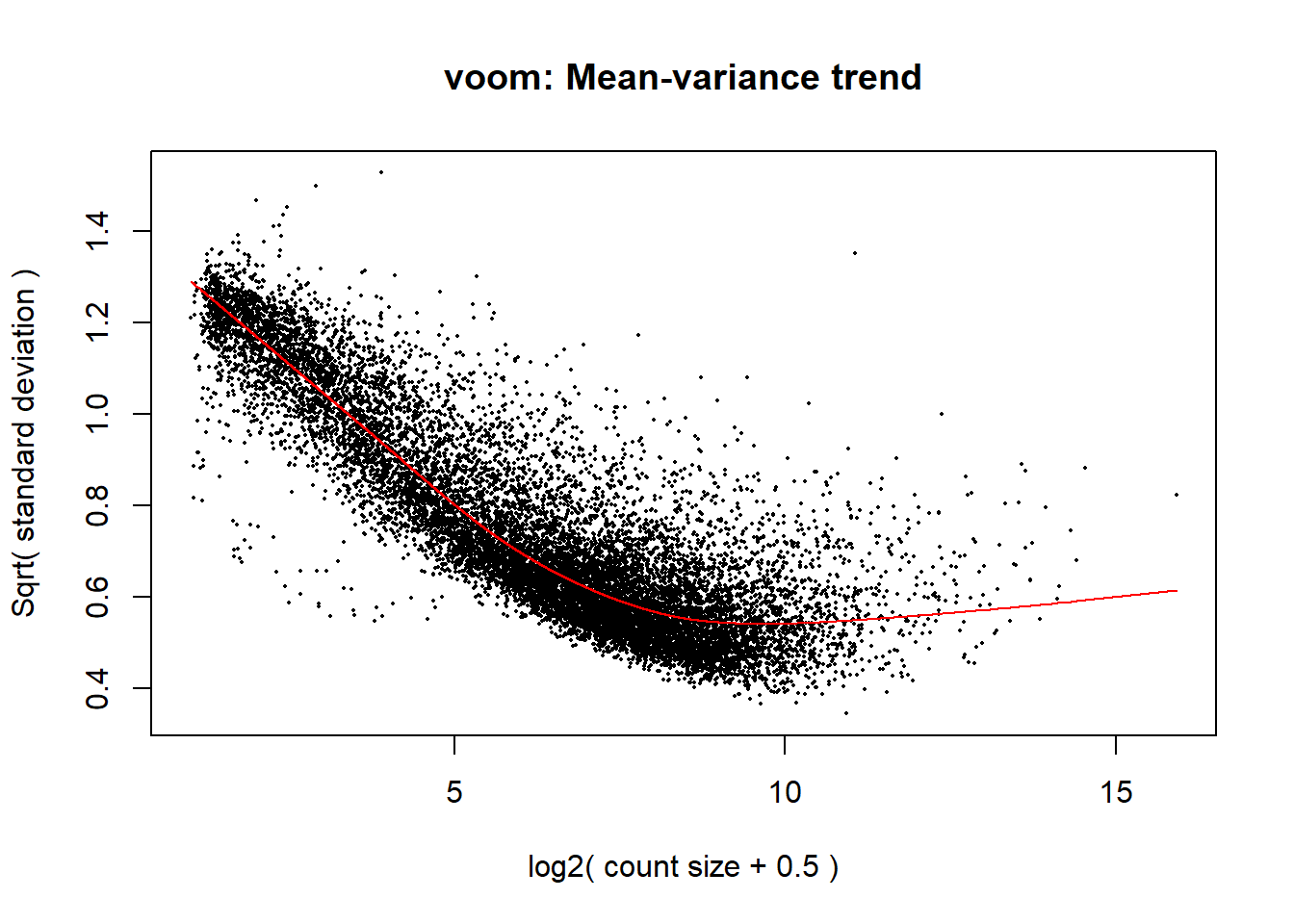
#fit my linear model
fit <- lmFit(v, design, block = meta_de$Ind,
             correlation = corfit$consensus.correlation)

#make my contrast matrix to compare across tx and veh within each species
contrast_matrix <- makeContrasts(
  V.TUN2_H = TUN_2_H - DMSO_2_H,
  V.THA2_H = THA_2_H - DMSO_2_H,
  V.TUN24_H = TUN_24_H - DMSO_24_H,
  V.THA24_H = THA_24_H - DMSO_24_H,
  V.DOX24_H = DOX_24_H - DMSO_24_H,
  V.NUTL24_H = NUTL_24_H - DMSO_24_H,
  V.LPS24_H = LPS_24_H - H2O_24_H,
  V.TNFa24_H = TNFa_24_H - H2O_24_H,
  V.BPA24_H = BPA_24_H - EtOH_24_H,
  V.PFOA24_H = PFOA_24_H - EtOH_24_H,
  V.TUN2_C = TUN_2_C - DMSO_2_C,
  V.THA2_C = THA_2_C - DMSO_2_C,
  V.TUN24_C = TUN_24_C - DMSO_24_C,
  V.THA24_C = THA_24_C - DMSO_24_C,
  V.DOX24_C = DOX_24_C - DMSO_24_C,
  V.NUTL24_C = NUTL_24_C - DMSO_24_C,
  V.LPS24_C = LPS_24_C - H2O_24_C,
  V.TNFa24_C = TNFa_24_C - H2O_24_C,
  V.BPA24_C = BPA_24_C - EtOH_24_C,
  V.PFOA24_C = PFOA_24_C - EtOH_24_C,
  levels = design
)

#apply these contrasts to compare stimuli to vehicle
fit2 <- contrasts.fit(fit, contrast_matrix)
fit2 <- eBayes(fit2)

#plot the mean-variance trend
plotSA(fit2, main = "final model: mean-variance trend")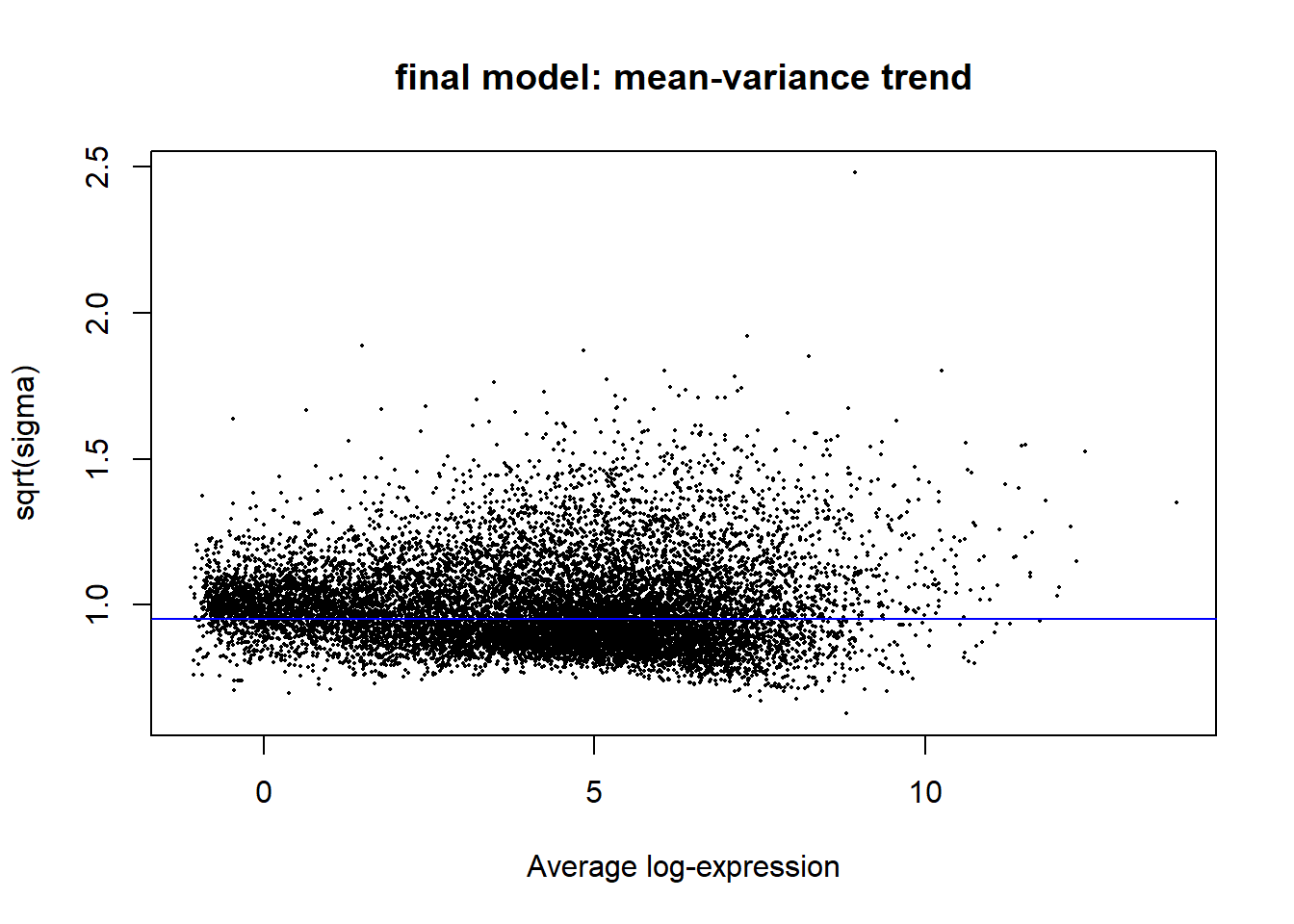
#now look at the summary of results to identify whether there are DEGs in each comparison
results_summary <- decideTests(fit2, adjust.method = "BH", p.value = 0.05)
summary(results_summary)
V.TUN2_H V.THA2_H V.TUN24_H V.THA24_H V.DOX24_H V.NUTL24_H V.LPS24_H
Down 0 660 1554 1917 4297 653 0
NotSig 13739 12364 10712 10051 5420 12440 13739
Up 0 715 1473 1771 4022 646 0
V.TNFa24_H V.BPA24_H V.PFOA24_H V.TUN2_C V.THA2_C V.TUN24_C V.THA24_C
Down 0 0 0 0 373 1662 1995
NotSig 13689 13739 13739 13739 12762 10574 9785
Up 50 0 0 0 604 1503 1959
V.DOX24_C V.NUTL24_C V.LPS24_C V.TNFa24_C V.BPA24_C V.PFOA24_C
Down 4329 497 0 15 0 0
NotSig 5341 12594 13727 13575 13739 13739
Up 4069 648 12 149 0 0Create Toptables
#2hr Human Toptables
Toptable_V.TUN2_H <- topTable(fit = fit2,
                            coef = "V.TUN2_H",
                            number = nrow(x),
                            adjust.method = "BH",
                            p.value = 1,
                            sort.by = "none")

Toptable_V.THA2_H <- topTable(fit = fit2,
                            coef = "V.THA2_H",
                            number = nrow(x),
                            adjust.method = "BH",
                            p.value = 1,
                            sort.by = "none")

#2hr Chimp Toptables
Toptable_V.TUN2_C <- topTable(fit = fit2,
                            coef = "V.TUN2_C",
                            number = nrow(x),
                            adjust.method = "BH",
                            p.value = 1,
                            sort.by = "none")

Toptable_V.THA2_C <- topTable(fit = fit2,
                            coef = "V.THA2_C",
                            number = nrow(x),
                            adjust.method = "BH",
                            p.value = 1,
                            sort.by = "none")

#24hr toptables human

Toptable_V.TUN24_H <- topTable(fit = fit2,
                            coef = "V.TUN24_H",
                            number = nrow(x),
                            adjust.method = "BH",
                            p.value = 1,
                            sort.by = "none")

Toptable_V.THA24_H <- topTable(fit = fit2,
                            coef = "V.THA24_H",
                            number = nrow(x),
                            adjust.method = "BH",
                            p.value = 1,
                            sort.by = "none")

Toptable_V.DOX24_H <- topTable(fit = fit2,
                            coef = "V.DOX24_H",
                            number = nrow(x),
                            adjust.method = "BH",
                            p.value = 1,
                            sort.by = "none")

Toptable_V.NUTL24_H <- topTable(fit = fit2,
                            coef = "V.NUTL24_H",
                            number = nrow(x),
                            adjust.method = "BH",
                            p.value = 1,
                            sort.by = "none")

Toptable_V.LPS24_H <- topTable(fit = fit2,
                            coef = "V.LPS24_H",
                            number = nrow(x),
                            adjust.method = "BH",
                            p.value = 1,
                            sort.by = "none")

Toptable_V.TNFa24_H <- topTable(fit = fit2,
                            coef = "V.TNFa24_H",
                            number = nrow(x),
                            adjust.method = "BH",
                            p.value = 1,
                            sort.by = "none")

Toptable_V.BPA24_H <- topTable(fit = fit2,
                            coef = "V.BPA24_H",
                            number = nrow(x),
                            adjust.method = "BH",
                            p.value = 1,
                            sort.by = "none")

Toptable_V.PFOA24_H <- topTable(fit = fit2,
                            coef = "V.PFOA24_H",
                            number = nrow(x),
                            adjust.method = "BH",
                            p.value = 1,
                            sort.by = "none")


#chimp 24hr toptables

Toptable_V.TUN24_C <- topTable(fit = fit2,
                            coef = "V.TUN24_C",
                            number = nrow(x),
                            adjust.method = "BH",
                            p.value = 1,
                            sort.by = "none")

Toptable_V.THA24_C <- topTable(fit = fit2,
                            coef = "V.THA24_C",
                            number = nrow(x),
                            adjust.method = "BH",
                            p.value = 1,
                            sort.by = "none")

Toptable_V.DOX24_C <- topTable(fit = fit2,
                            coef = "V.DOX24_C",
                            number = nrow(x),
                            adjust.method = "BH",
                            p.value = 1,
                            sort.by = "none")

Toptable_V.NUTL24_C <- topTable(fit = fit2,
                            coef = "V.NUTL24_C",
                            number = nrow(x),
                            adjust.method = "BH",
                            p.value = 1,
                            sort.by = "none")

Toptable_V.LPS24_C <- topTable(fit = fit2,
                            coef = "V.LPS24_C",
                            number = nrow(x),
                            adjust.method = "BH",
                            p.value = 1,
                            sort.by = "none")

Toptable_V.TNFa24_C <- topTable(fit = fit2,
                            coef = "V.TNFa24_C",
                            number = nrow(x),
                            adjust.method = "BH",
                            p.value = 1,
                            sort.by = "none")

Toptable_V.BPA24_C <- topTable(fit = fit2,
                            coef = "V.BPA24_C",
                            number = nrow(x),
                            adjust.method = "BH",
                            p.value = 1,
                            sort.by = "none")

Toptable_V.PFOA24_C <- topTable(fit = fit2,
                            coef = "V.PFOA24_C",
                            number = nrow(x),
                            adjust.method = "BH",
                            p.value = 1,
                            sort.by = "none")
sessionInfo()R version 4.4.2 (2024-10-31 ucrt)
Platform: x86_64-w64-mingw32/x64
Running under: Windows 11 x64 (build 22000)
Matrix products: default
locale:
[1] LC_COLLATE=English_United States.utf8
[2] LC_CTYPE=English_United States.utf8
[3] LC_MONETARY=English_United States.utf8
[4] LC_NUMERIC=C
[5] LC_TIME=English_United States.utf8
time zone: America/Chicago
tzcode source: internal
attached base packages:
[1] grid stats4 stats graphics grDevices utils datasets
[8] methods base
other attached packages:
[1] magick_2.9.0 broom_1.0.8
[3] gprofiler2_0.2.3 car_3.1-3
[5] carData_3.0-5 patchwork_1.3.0
[7] eulerr_7.0.2 ggrastr_1.0.2
[9] rstatix_0.7.2 ggsignif_0.6.4
[11] RUVSeq_1.40.0 EDASeq_2.40.0
[13] ShortRead_1.64.0 GenomicAlignments_1.42.0
[15] SummarizedExperiment_1.36.0 MatrixGenerics_1.18.1
[17] matrixStats_1.5.0 Rsamtools_2.22.0
[19] GenomicRanges_1.58.0 Biostrings_2.74.0
[21] GenomeInfoDb_1.42.3 XVector_0.46.0
[23] BiocParallel_1.40.0 VennDetail_1.22.0
[25] VennDiagram_1.7.3 futile.logger_1.4.3
[27] ggpubr_0.6.0 UpSetR_1.4.0
[29] ggVennDiagram_1.5.2 reshape2_1.4.4
[31] circlize_0.4.16 ComplexHeatmap_2.22.0
[33] org.Hs.eg.db_3.20.0 AnnotationDbi_1.68.0
[35] IRanges_2.40.0 S4Vectors_0.44.0
[37] corrplot_0.95 ggfortify_0.4.17
[39] ggrepel_0.9.6 biomaRt_2.62.1
[41] scales_1.4.0 edgebundleR_0.1.4
[43] edgeR_4.4.0 limma_3.62.1
[45] Biobase_2.66.0 BiocGenerics_0.52.0
[47] lubridate_1.9.4 forcats_1.0.0
[49] stringr_1.5.1 dplyr_1.1.4
[51] purrr_1.0.4 readr_2.1.5
[53] tidyr_1.3.1 tibble_3.2.1
[55] ggplot2_3.5.2 tidyverse_2.0.0
[57] workflowr_1.7.1
loaded via a namespace (and not attached):
[1] later_1.4.2 BiocIO_1.16.0 bitops_1.0-9
[4] filelock_1.0.3 R.oo_1.27.1 XML_3.99-0.18
[7] lifecycle_1.0.4 httr2_1.1.2 pwalign_1.2.0
[10] doParallel_1.0.17 rprojroot_2.0.4 vroom_1.6.5
[13] MASS_7.3-61 processx_3.8.6 lattice_0.22-6
[16] backports_1.5.0 magrittr_2.0.3 plotly_4.10.4
[19] sass_0.4.10 rmarkdown_2.29 jquerylib_0.1.4
[22] yaml_2.3.10 httpuv_1.6.16 DBI_1.2.3
[25] RColorBrewer_1.1-3 abind_1.4-8 zlibbioc_1.52.0
[28] R.utils_2.13.0 RCurl_1.98-1.17 rappdirs_0.3.3
[31] git2r_0.36.2 GenomeInfoDbData_1.2.13 codetools_0.2-20
[34] DelayedArray_0.32.0 xml2_1.3.8 tidyselect_1.2.1
[37] shape_1.4.6.1 UCSC.utils_1.2.0 farver_2.1.2
[40] BiocFileCache_2.14.0 jsonlite_2.0.0 GetoptLong_1.0.5
[43] Formula_1.2-5 iterators_1.0.14 foreach_1.5.2
[46] tools_4.4.2 progress_1.2.3 Rcpp_1.0.14
[49] glue_1.8.0 gridExtra_2.3 SparseArray_1.6.0
[52] xfun_0.52 withr_3.0.2 formatR_1.14
[55] fastmap_1.2.0 latticeExtra_0.6-30 callr_3.7.6
[58] digest_0.6.37 timechange_0.3.0 R6_2.6.1
[61] mime_0.13 colorspace_2.1-1 jpeg_0.1-11
[64] RSQLite_2.3.9 R.methodsS3_1.8.2 generics_0.1.4
[67] data.table_1.17.0 rtracklayer_1.66.0 prettyunits_1.2.0
[70] httr_1.4.7 htmlwidgets_1.6.4 S4Arrays_1.6.0
[73] whisker_0.4.1 pkgconfig_2.0.3 gtable_0.3.6
[76] blob_1.2.4 hwriter_1.3.2.1 htmltools_0.5.8.1
[79] clue_0.3-66 png_0.1-8 knitr_1.50
[82] lambda.r_1.2.4 rstudioapi_0.17.1 tzdb_0.5.0
[85] rjson_0.2.23 curl_6.0.1 cachem_1.1.0
[88] GlobalOptions_0.1.2 vipor_0.4.7 parallel_4.4.2
[91] restfulr_0.0.15 pillar_1.10.2 vctrs_0.6.5
[94] promises_1.3.2 dbplyr_2.5.0 xtable_1.8-4
[97] cluster_2.1.6 beeswarm_0.4.0 evaluate_1.0.3
[100] GenomicFeatures_1.58.0 cli_3.6.3 locfit_1.5-9.12
[103] compiler_4.4.2 futile.options_1.0.1 rlang_1.1.6
[106] crayon_1.5.3 aroma.light_3.36.0 interp_1.1-6
[109] ps_1.9.1 ggbeeswarm_0.7.2 getPass_0.2-4
[112] plyr_1.8.9 fs_1.6.6 stringi_1.8.7
[115] viridisLite_0.4.2 deldir_2.0-4 lazyeval_0.2.2
[118] Matrix_1.7-1 hms_1.1.3 bit64_4.5.2
[121] KEGGREST_1.46.0 statmod_1.5.0 shiny_1.10.0
[124] igraph_2.1.4 memoise_2.0.1 bslib_0.9.0
[127] bit_4.5.0