5FU Recovery RNAseq Analysis
Emma M Pfortmiller
2025-02-10
Last updated: 2025-02-27
Checks: 7 0
Knit directory: Recovery_5FU/
This reproducible R Markdown analysis was created with workflowr (version 1.7.1). The Checks tab describes the reproducibility checks that were applied when the results were created. The Past versions tab lists the development history.
Great! Since the R Markdown file has been committed to the Git repository, you know the exact version of the code that produced these results.
Great job! The global environment was empty. Objects defined in the global environment can affect the analysis in your R Markdown file in unknown ways. For reproduciblity it’s best to always run the code in an empty environment.
The command set.seed(20250217) was run prior to running
the code in the R Markdown file. Setting a seed ensures that any results
that rely on randomness, e.g. subsampling or permutations, are
reproducible.
Great job! Recording the operating system, R version, and package versions is critical for reproducibility.
Nice! There were no cached chunks for this analysis, so you can be confident that you successfully produced the results during this run.
Great job! Using relative paths to the files within your workflowr project makes it easier to run your code on other machines.
Great! You are using Git for version control. Tracking code development and connecting the code version to the results is critical for reproducibility.
The results in this page were generated with repository version e77e0d4. See the Past versions tab to see a history of the changes made to the R Markdown and HTML files.
Note that you need to be careful to ensure that all relevant files for
the analysis have been committed to Git prior to generating the results
(you can use wflow_publish or
wflow_git_commit). workflowr only checks the R Markdown
file, but you know if there are other scripts or data files that it
depends on. Below is the status of the Git repository when the results
were generated:
Ignored files:
    Ignored:    .Rhistory
    Ignored:    .Rproj.user/

Untracked files:
    Untracked:  code/Recovery_RNAseq_Analysis_EMP_250210.Rmd

Unstaged changes:
    Deleted:    analysis/Recovery_RNAseq_Analysis_EMP_250210.Rmd
Note that any generated files, e.g. HTML, png, CSS, etc., are not included in this status report because it is ok for generated content to have uncommitted changes.
These are the previous versions of the repository in which changes were
made to the R Markdown (analysis/Recovery_DE.Rmd) and HTML
(docs/Recovery_DE.html) files. If you’ve configured a
remote Git repository (see ?wflow_git_remote), click on the
hyperlinks in the table below to view the files as they were in that
past version.
| File | Version | Author | Date | Message |
|---|---|---|---|---|
| Rmd | e77e0d4 | emmapfort | 2025-02-27 | Make website cohesive and dataframes concise. |
Welcome to my research website.
── Attaching core tidyverse packages ──────────────────────── tidyverse 2.0.0 ──
✔ dplyr     1.1.4     ✔ readr     2.1.5
✔ forcats   1.0.0     ✔ stringr   1.5.1
✔ lubridate 1.9.3     ✔ tidyr     1.3.1
✔ purrr     1.0.2
── Conflicts ────────────────────────────────────────── tidyverse_conflicts() ──
✖ dplyr::filter() masks stats::filter()
✖ dplyr::lag()    masks stats::lag()
ℹ Use the conflicted package (<http://conflicted.r-lib.org/>) to force all conflicts to become errors
Loading required package: limma

Loading required package: ggrepel


Attaching package: 'PCAtools'


The following objects are masked from 'package:stats':

    biplot, screeplot


Loading required package: affy

Loading required package: BiocGenerics


Attaching package: 'BiocGenerics'


The following object is masked from 'package:limma':

    plotMA


The following objects are masked from 'package:lubridate':

    intersect, setdiff, union


The following objects are masked from 'package:dplyr':

    combine, intersect, setdiff, union


The following objects are masked from 'package:stats':

    IQR, mad, sd, var, xtabs


The following objects are masked from 'package:base':

    anyDuplicated, aperm, append, as.data.frame, basename, cbind,
    colnames, dirname, do.call, duplicated, eval, evalq, Filter, Find,
    get, grep, grepl, intersect, is.unsorted, lapply, Map, mapply,
    match, mget, order, paste, pmax, pmax.int, pmin, pmin.int,
    Position, rank, rbind, Reduce, rownames, sapply, saveRDS, setdiff,
    table, tapply, union, unique, unsplit, which.max, which.min


Loading required package: Biobase

Welcome to Bioconductor

    Vignettes contain introductory material; view with
    'browseVignettes()'. To cite Bioconductor, see
    'citation("Biobase")', and for packages 'citation("pkgname")'.


Attaching package: 'affy'


The following object is masked from 'package:lubridate':

    pm


Loading required package: EDASeq

Loading required package: ShortRead

Loading required package: BiocParallel

Loading required package: Biostrings

Loading required package: S4Vectors

Loading required package: stats4


Attaching package: 'S4Vectors'


The following objects are masked from 'package:lubridate':

    second, second<-


The following objects are masked from 'package:dplyr':

    first, rename


The following object is masked from 'package:tidyr':

    expand


The following object is masked from 'package:utils':

    findMatches


The following objects are masked from 'package:base':

    expand.grid, I, unname


Loading required package: IRanges


Attaching package: 'IRanges'


The following object is masked from 'package:lubridate':

    %within%


The following objects are masked from 'package:dplyr':

    collapse, desc, slice


The following object is masked from 'package:purrr':

    reduce


The following object is masked from 'package:grDevices':

    windows


Loading required package: XVector


Attaching package: 'XVector'


The following object is masked from 'package:purrr':

    compact


Loading required package: GenomeInfoDb


Attaching package: 'Biostrings'


The following object is masked from 'package:base':

    strsplit


Loading required package: Rsamtools

Loading required package: GenomicRanges

Loading required package: GenomicAlignments

Loading required package: SummarizedExperiment

Loading required package: MatrixGenerics

Loading required package: matrixStats


Attaching package: 'matrixStats'


The following objects are masked from 'package:Biobase':

    anyMissing, rowMedians


The following object is masked from 'package:dplyr':

    count


Attaching package: 'MatrixGenerics'


The following objects are masked from 'package:matrixStats':

    colAlls, colAnyNAs, colAnys, colAvgsPerRowSet, colCollapse,
    colCounts, colCummaxs, colCummins, colCumprods, colCumsums,
    colDiffs, colIQRDiffs, colIQRs, colLogSumExps, colMadDiffs,
    colMads, colMaxs, colMeans2, colMedians, colMins, colOrderStats,
    colProds, colQuantiles, colRanges, colRanks, colSdDiffs, colSds,
    colSums2, colTabulates, colVarDiffs, colVars, colWeightedMads,
    colWeightedMeans, colWeightedMedians, colWeightedSds,
    colWeightedVars, rowAlls, rowAnyNAs, rowAnys, rowAvgsPerColSet,
    rowCollapse, rowCounts, rowCummaxs, rowCummins, rowCumprods,
    rowCumsums, rowDiffs, rowIQRDiffs, rowIQRs, rowLogSumExps,
    rowMadDiffs, rowMads, rowMaxs, rowMeans2, rowMedians, rowMins,
    rowOrderStats, rowProds, rowQuantiles, rowRanges, rowRanks,
    rowSdDiffs, rowSds, rowSums2, rowTabulates, rowVarDiffs, rowVars,
    rowWeightedMads, rowWeightedMeans, rowWeightedMedians,
    rowWeightedSds, rowWeightedVars


The following object is masked from 'package:Biobase':

    rowMedians


Attaching package: 'GenomicAlignments'


The following object is masked from 'package:dplyr':

    last


Attaching package: 'ShortRead'


The following object is masked from 'package:affy':

    intensity


The following object is masked from 'package:dplyr':

    id


The following object is masked from 'package:purrr':

    compose


The following object is masked from 'package:tibble':

    view
These samples (63 in total) have been aligned to the Ensembl 113 release of GRCh38 via subread, and counts have been generated using featureCounts with inbuilt hg38 genome
Data is located under 5FU Project on my computer All analysis saved in RDirectory Recovery_RNAseq
Individual 1 - 84-1 (9 samples)
Individual 2 - 87-1 (9 samples)
Individual 3 - 75-1 (9 samples)
Individual 4 - 75-1 (9 samples)
Individual 5 - 17-3 (9 samples)
Individual 6 - 90-1 (9 samples)
Individual 7 - 90-1 REP (9 samples)
Now that I have imported all of these counts files, I will make a matrix with all of the samples
First I’ll break them up by individual, and then combine them all together
Now that I’ve made individual matrices for each individual - I will combine them together into one large matrix
#Now that I've put together my matrix - I will do some QC checks

#now that I have all of my factors and my gene info, I will make some graphs to show the QC data

reads_by_sample <- c(tx_col)
fC_AllCounts %>%
  ggplot(., aes (x = Conditions, y = Total_Align, fill = Treatment, group_by = Line))+
  geom_col()+
 geom_hline(aes(yintercept=20000000))+
 scale_fill_manual(values=reads_by_sample)+
  ggtitle(expression("Total number of reads by sample"))+
  xlab("")+
  ylab(expression("RNA-sequencing reads"))+
  theme_bw()+
  theme(plot.title = element_text(size = rel(2), hjust = 0.5),
        axis.title = element_text(size = 15, color = "black"),
        axis.ticks = element_line(linewidth = 1.5),
        axis.line = element_line(linewidth = 1.5),
        axis.text.y = element_text(size =10, color = "black", angle = 0, hjust = 0.8, vjust = 0.5),
        axis.text.x = element_text(size =10, color = "black", angle = 90, hjust = 1, vjust = 0.2),
        #strip.text.x = element_text(size = 15, color = "black", face = "bold"),
        strip.text.y = element_text(color = "white"))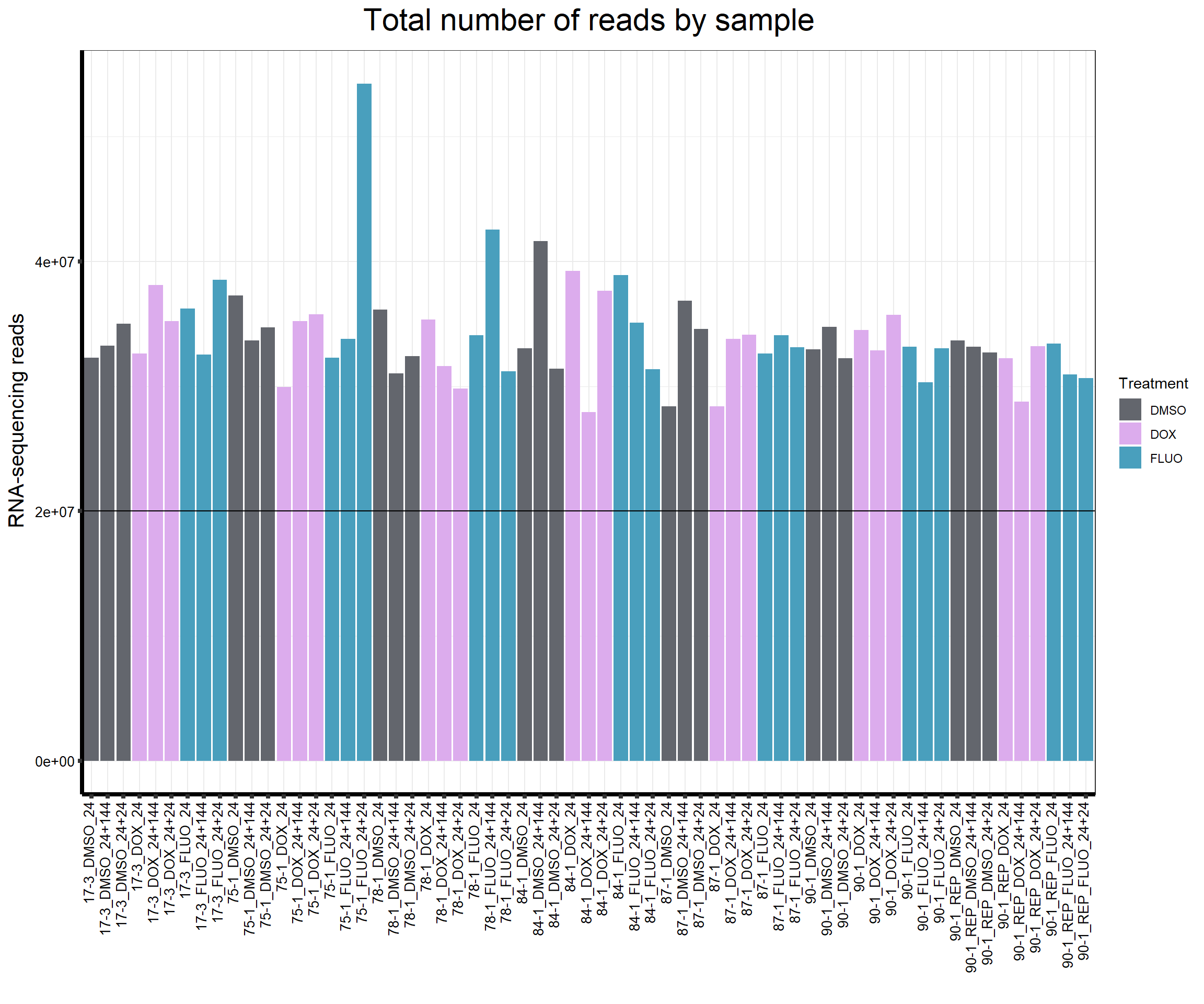
####Read Counts by Treatment####
fC_AllCounts %>%
  ggplot(., aes (x =Treatment, y= Total_Align, fill = Treatment))+
  geom_boxplot()+
 scale_fill_manual(values=reads_by_sample)+
  ggtitle(expression("Total number of reads by treatment"))+
  xlab("")+
  ylab(expression("RNA-sequencing reads"))+
  theme_bw()+

  theme(plot.title = element_text(size = rel(2), hjust = 0.5),
        axis.title = element_text(size = 15, color = "black"),
        axis.ticks = element_line(linewidth = 1.5),
        axis.line = element_line(linewidth = 1.5),
        axis.text.y = element_text(size =10, color = "black", angle = 0, hjust = 0.8, vjust = 0.5),
        axis.text.x = element_text(size =10, color = "black", angle = 90, hjust = 1, vjust = 0.2),
        #strip.text.x = element_text(size = 15, color = "black", face = "bold"),
        strip.text.y = element_text(color = "white"))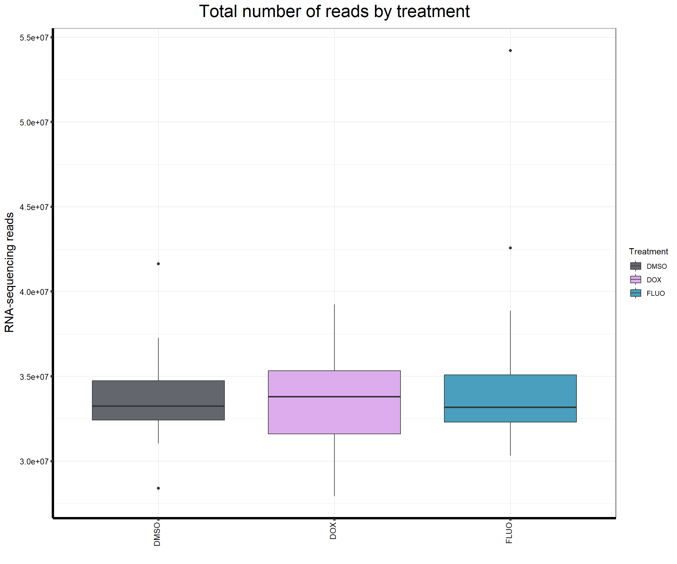
####Total Reads Per Individual####
fC_AllCounts %>%
  ggplot(., aes (x =as.factor(Line), y=Total_Align))+
  geom_boxplot(aes(fill=as.factor(Line)))+
 scale_fill_brewer(palette = "Dark2", name = "Individual")+
  ggtitle(expression("Total number of reads by individual"))+
  xlab("")+
  ylab(expression("RNA-sequencing reads"))+
  theme_bw()+

  theme(plot.title = element_text(size = rel(2), hjust = 0.5),
        axis.title = element_text(size = 15, color = "black"),
        axis.ticks = element_line(linewidth = 1.5),
        axis.line = element_line(linewidth = 1.5),
        axis.text.y = element_text(size =10, color = "black", angle = 0, hjust = 0.8, vjust = 0.5),
        axis.text.x = element_text(size =10, color = "black", angle = 0, hjust = 1),
        #strip.text.x = element_text(size = 15, color = "black", face = "bold"),
        strip.text.y = element_text(color = "white"))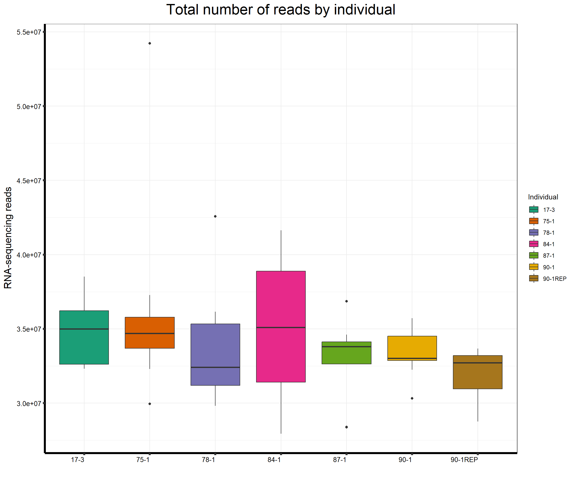
####Total Mapped Reads Per Drug####

reads_by_sample <- c(tx_col)
fC_AllCounts %>%
  ggplot(., aes (x = Conditions, y = Assigned_Align, fill = Treatment, group_by = Line))+
  geom_col()+
 geom_hline(aes(yintercept=20000000))+
 scale_fill_manual(values=reads_by_sample)+
  ggtitle(expression("Total number of mapped reads by sample"))+
  xlab("")+
  ylab(expression("RNA-sequencing reads"))+
  theme_bw()+
  theme(plot.title = element_text(size = rel(2), hjust = 0.5),
        axis.title = element_text(size = 15, color = "black"),
        axis.ticks = element_line(linewidth = 1.5),
        axis.line = element_line(linewidth = 1.5),
        axis.text.y = element_text(size =10, color = "black", angle = 0, hjust = 0.8, vjust = 0.5),
        axis.text.x = element_text(size =10, color = "black", angle = 90, hjust = 1, vjust = 0.2),
        #strip.text.x = element_text(size = 15, color = "black", face = "bold"),
        strip.text.y = element_text(color = "white"))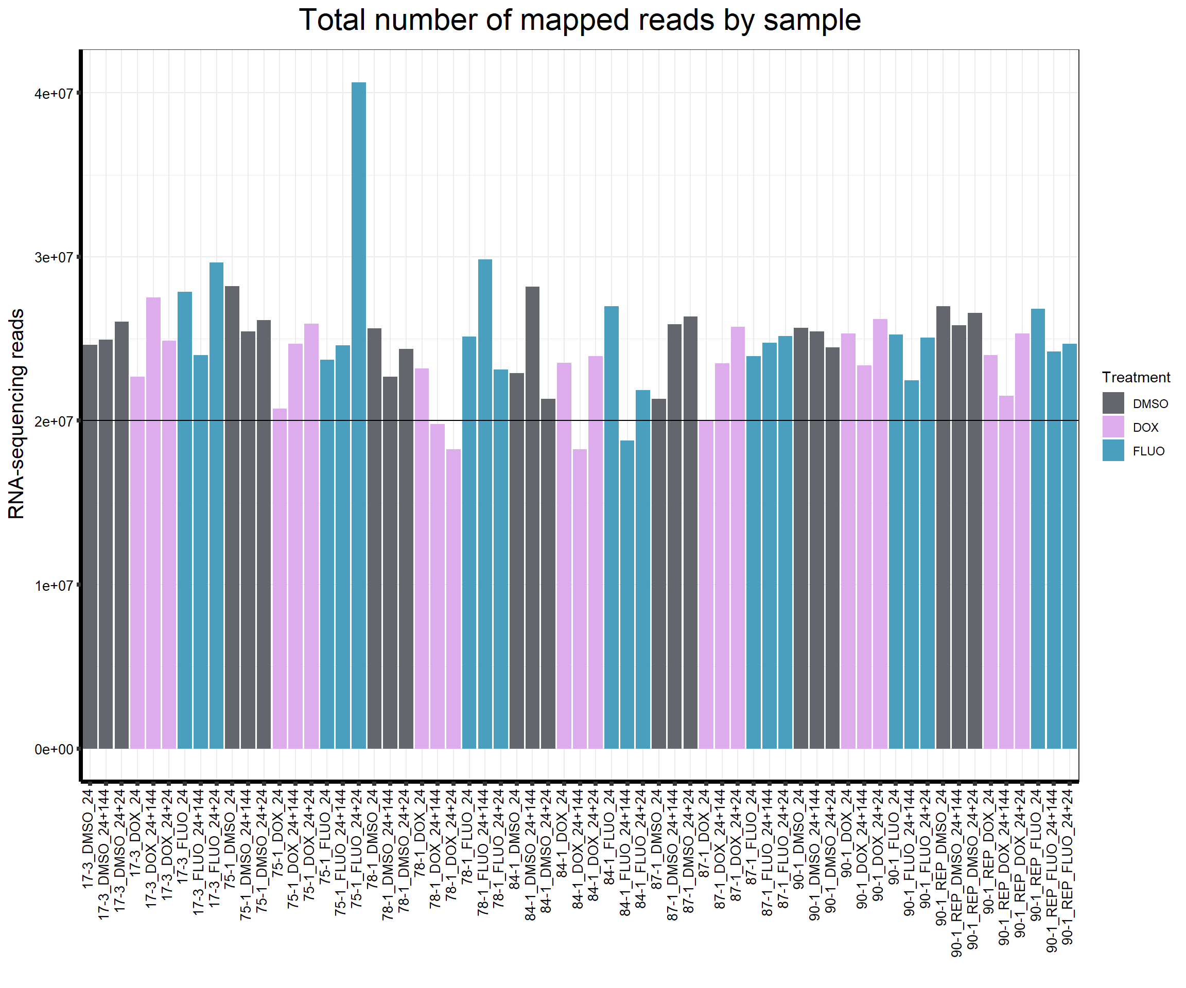
####Read Counts by Treatment####
fC_AllCounts %>%
  ggplot(., aes (x =Treatment, y= Assigned_Align, fill = Treatment))+
  geom_boxplot()+
 scale_fill_manual(values=reads_by_sample)+
  ggtitle(expression("Total number of mapped reads by treatment"))+
  xlab("")+
  ylab(expression("RNA-sequencing reads"))+
  theme_bw()+

  theme(plot.title = element_text(size = rel(2), hjust = 0.5),
        axis.title = element_text(size = 15, color = "black"),
        axis.ticks = element_line(linewidth = 1.5),
        axis.line = element_line(linewidth = 1.5),
        axis.text.y = element_text(size =10, color = "black", angle = 0, hjust = 0.8, vjust = 0.5),
        axis.text.x = element_text(size =10, color = "black", angle = 90, hjust = 1, vjust = 0.2),
        #strip.text.x = element_text(size = 15, color = "black", face = "bold"),
        strip.text.y = element_text(color = "white"))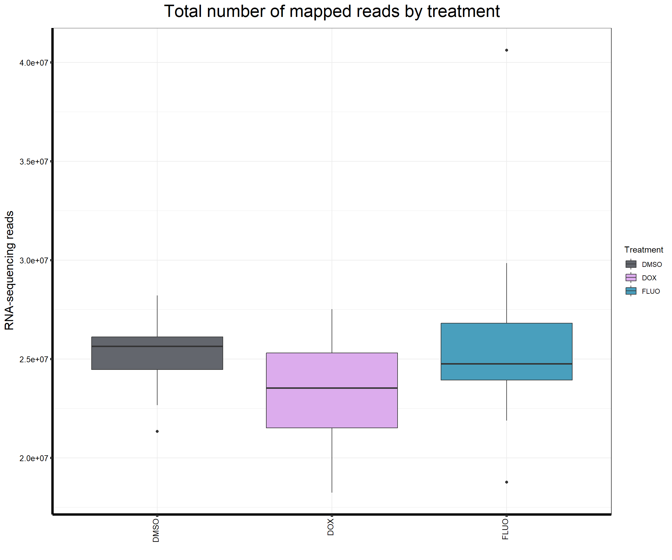
####Total Reads Per Individual####
fC_AllCounts %>%
  ggplot(., aes (x =as.factor(Line), y=Assigned_Align))+
  geom_boxplot(aes(fill=as.factor(Line)))+
 scale_fill_brewer(palette = "Dark2", name = "Individual")+
  ggtitle(expression("Total number of mapped reads by individual"))+
  xlab("")+
  ylab(expression("RNA-sequencing reads"))+
  theme_bw()+

  theme(plot.title = element_text(size = rel(2), hjust = 0.5),
        axis.title = element_text(size = 15, color = "black"),
        axis.ticks = element_line(linewidth = 1.5),
        axis.line = element_line(linewidth = 1.5),
        axis.text.y = element_text(size =10, color = "black", angle = 0, hjust = 0.8, vjust = 0.5),
        axis.text.x = element_text(size =10, color = "black", angle = 0, hjust = 1),
        #strip.text.x = element_text(size = 15, color = "black", face = "bold"),
        strip.text.y = element_text(color = "white"))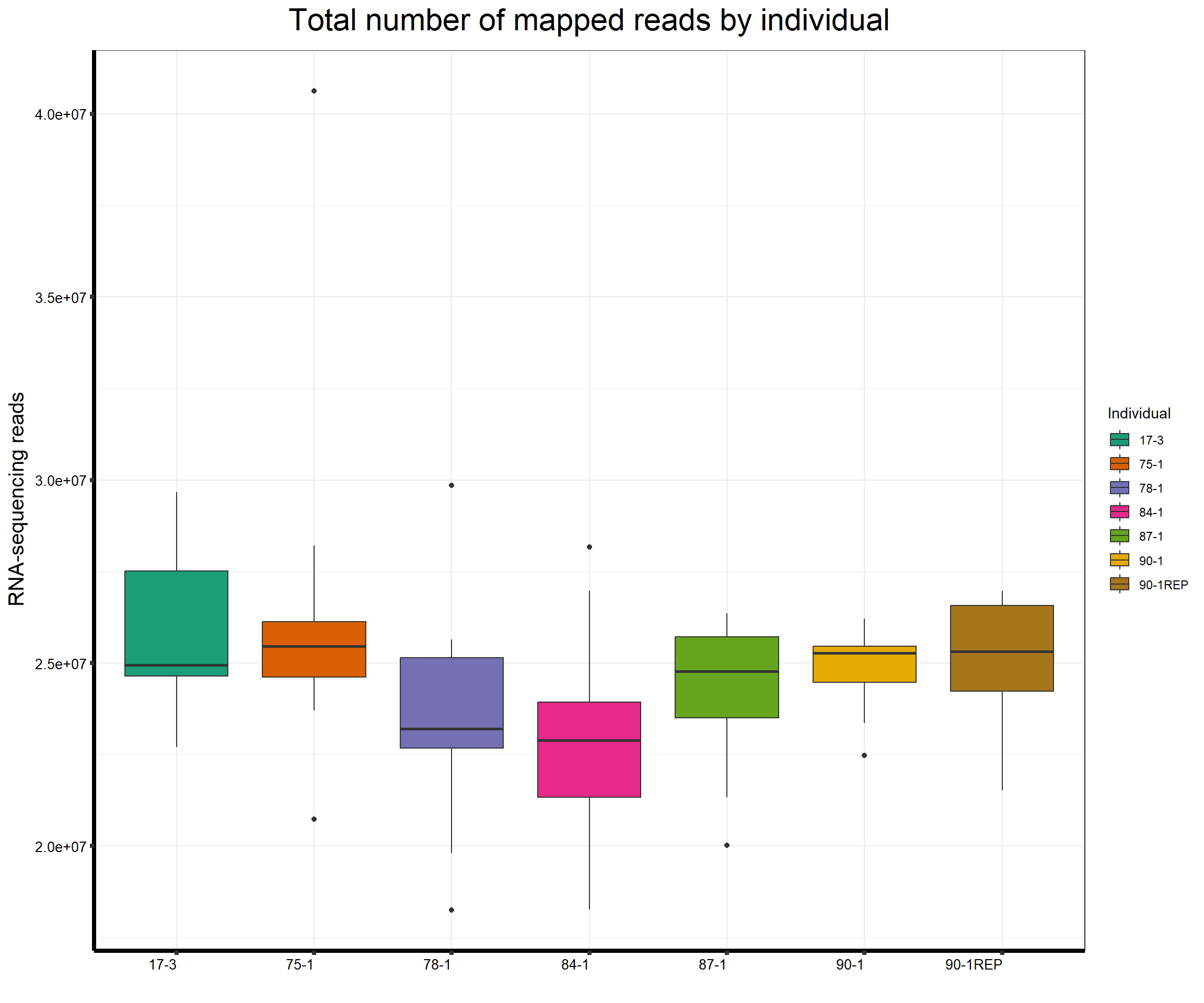
Now that I’ve made the final full matrix of all samples - 1. convert to log2cpm using cpm 2. filter for lowly expressed reads (rowMeans > 0)
boxplot(fC_Matrix_Full_cpm, xlab = "Conditions", ylab = expression("log"[2]* "counts per million"), ylim= c(-10, 20))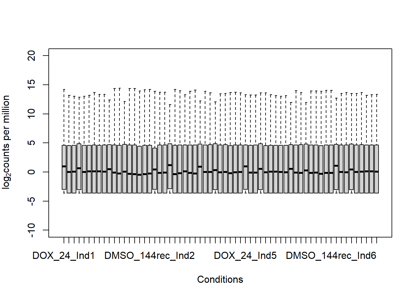
hist(fC_Matrix_Full_cpm, xlab = expression("log" [2]* "counts per million"))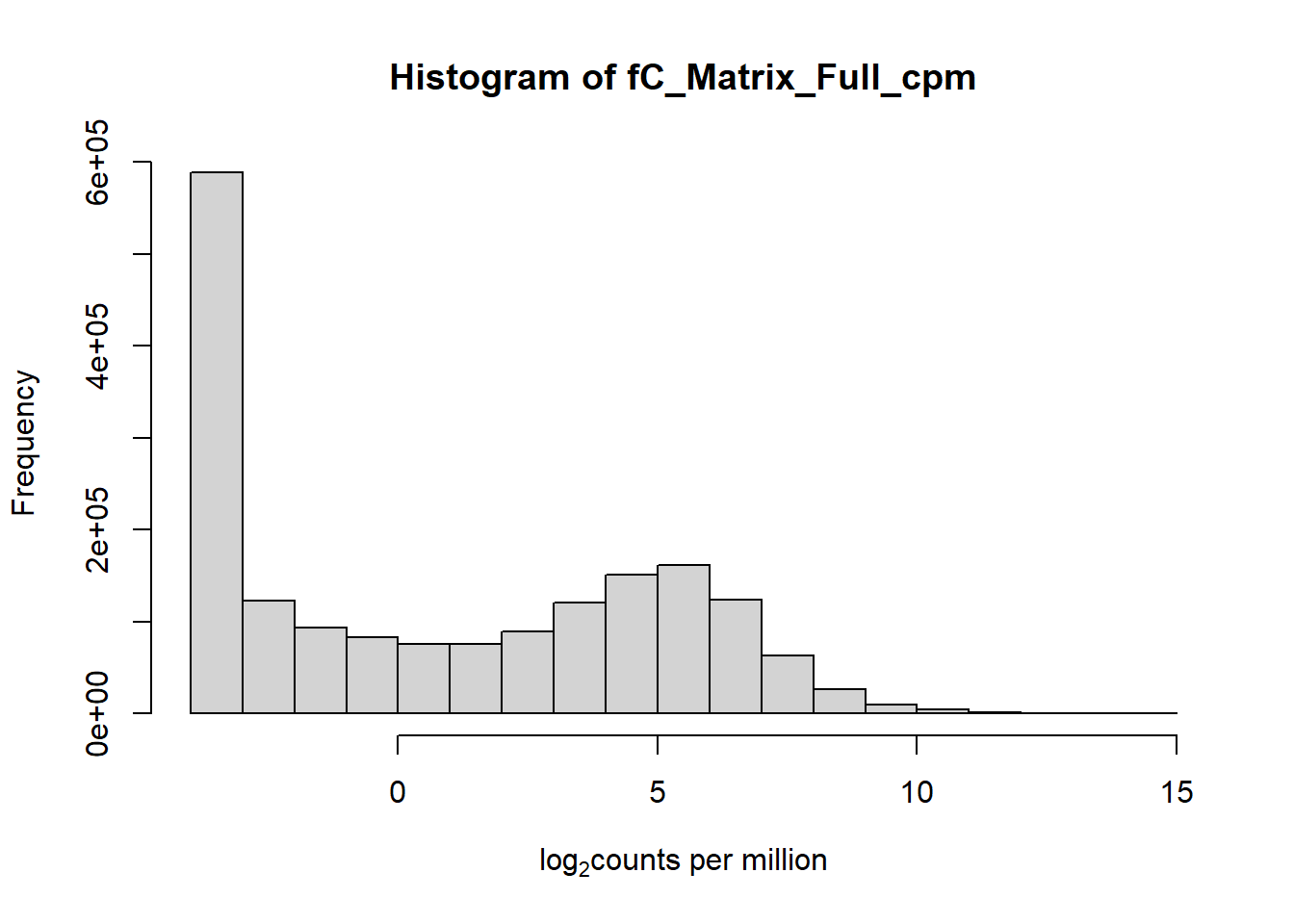
#write this to a csv just in case to save it
#write.csv(fC_Matrix_Full_cpm, "C:/Users/emmap/RDirectory/Recovery_RNAseq/Recovery_RNAseq/featureCounts_Concat_Matrix_AllSamples_cpm_EMP_250210.csv")
#first check the number of variables in the cpm file
dim(fC_Matrix_Full_cpm)
[1] 28395    63
#[1] 28395    63

#now use rowMeans to filter out values with mean < 0 (this means rowMeans > 0 is what I'm left with) for each row/gene in the original file
rowMeans_All <- rowMeans(fC_Matrix_Full_cpm)
fC_Matrix_Full_cpm_filter <- fC_Matrix_Full_cpm[rowMeans_All > 0,]
dim(fC_Matrix_Full_cpm_filter)
[1] 14225    63
#[1] 14225    63

#with this I've filtered out a significant number of rows when filtering after cpm conversion - does this make it more balanced?

hist(fC_Matrix_Full_cpm_filter,
     main = "Recovery All Individuals log2cpm Filtered",
        xlab = expression("log"[2]*"counts per million"))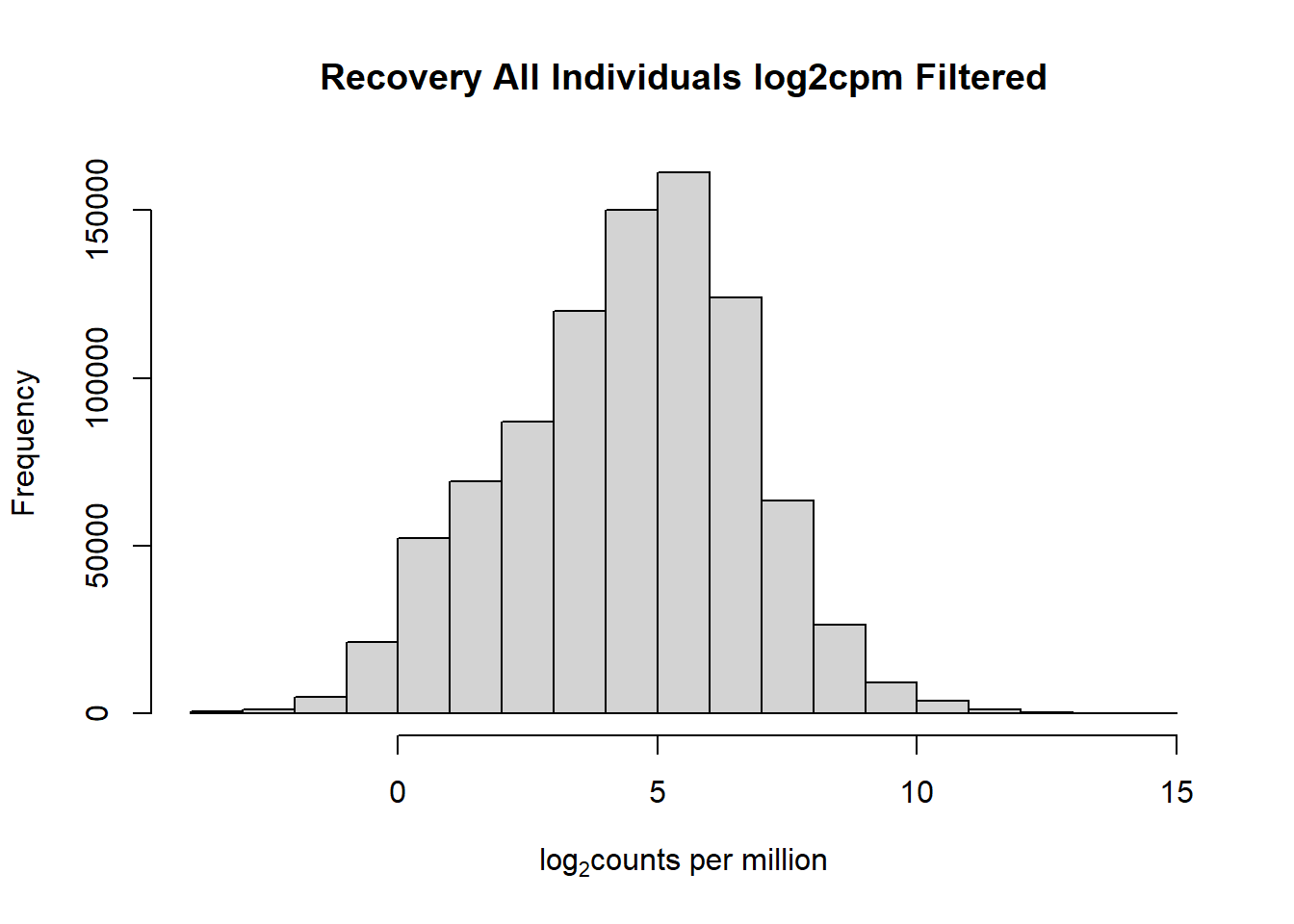
boxplot(fC_Matrix_Full_cpm_filter,
        main = "Recovery All Individuals log2cpm Filtered",
        xlab = "Conditions",
        ylab = expression("log"[2]*"counts per million"),
        ylim = c(-10,15))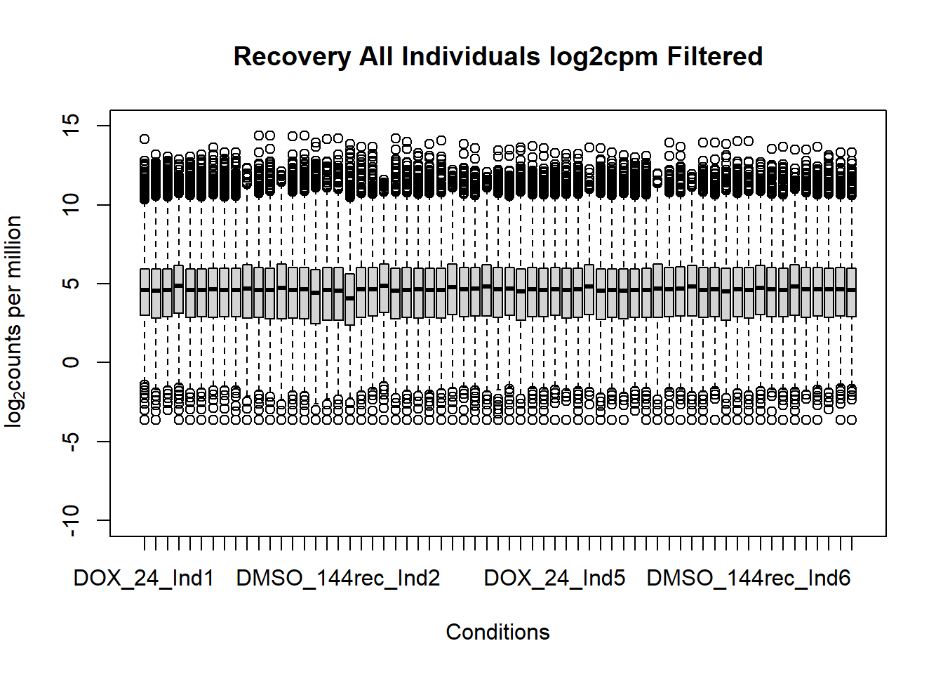
#write this to a csv to save
#write.csv(fC_Matrix_Full_cpm_filter, "C:/Users/emmap/RDirectory/Recovery_RNAseq/Recovery_RNAseq/featureCounts_Concat_Matrix_AllSamples_cpm_filtered_EMP_250210.csv")
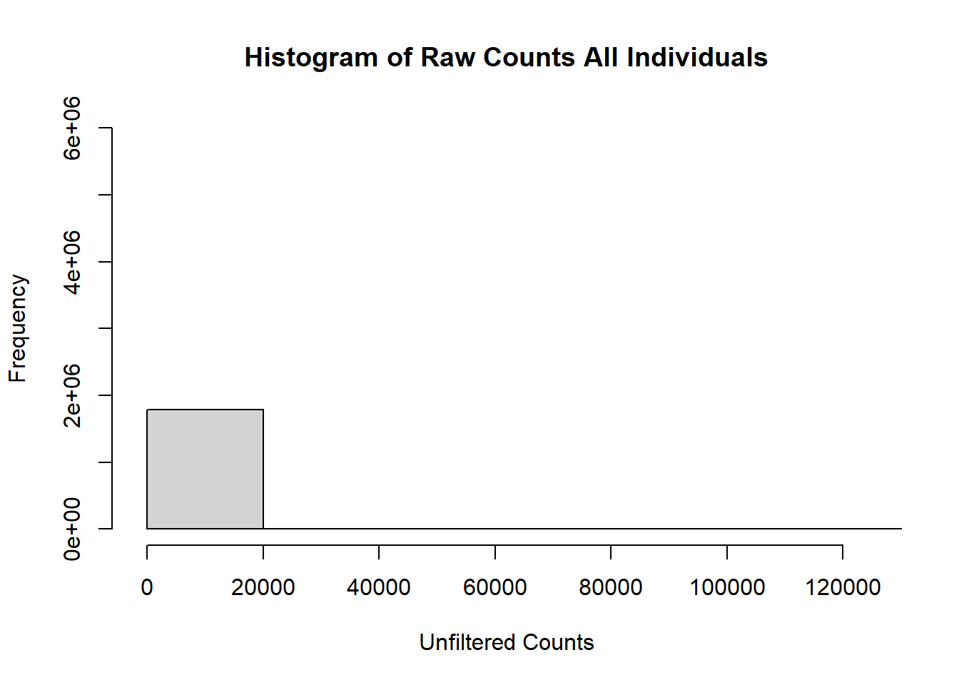
####histogram of total counts, unfiltered####
hist(fC_Matrix_Full_cpm, main = "Recovery All Individuals log2cpm Unfiltered",
     xlab = expression("log" [2]* "counts per million"))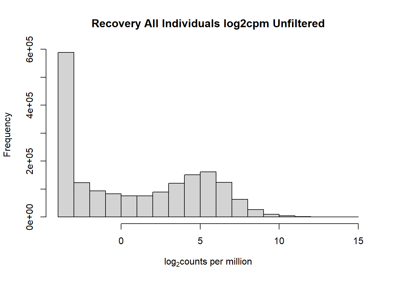
####histogram of total counts, filtered####
hist(fC_Matrix_Full_cpm_filter,
     main = "Recovery All Individuals log2cpm Filtered rowMeans > 0",
        xlab = expression("log"[2]*"counts per million"))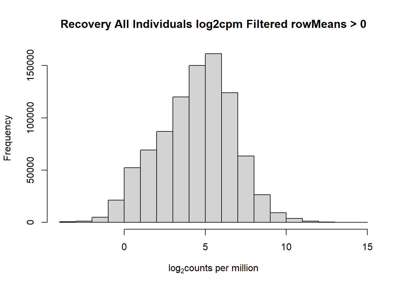
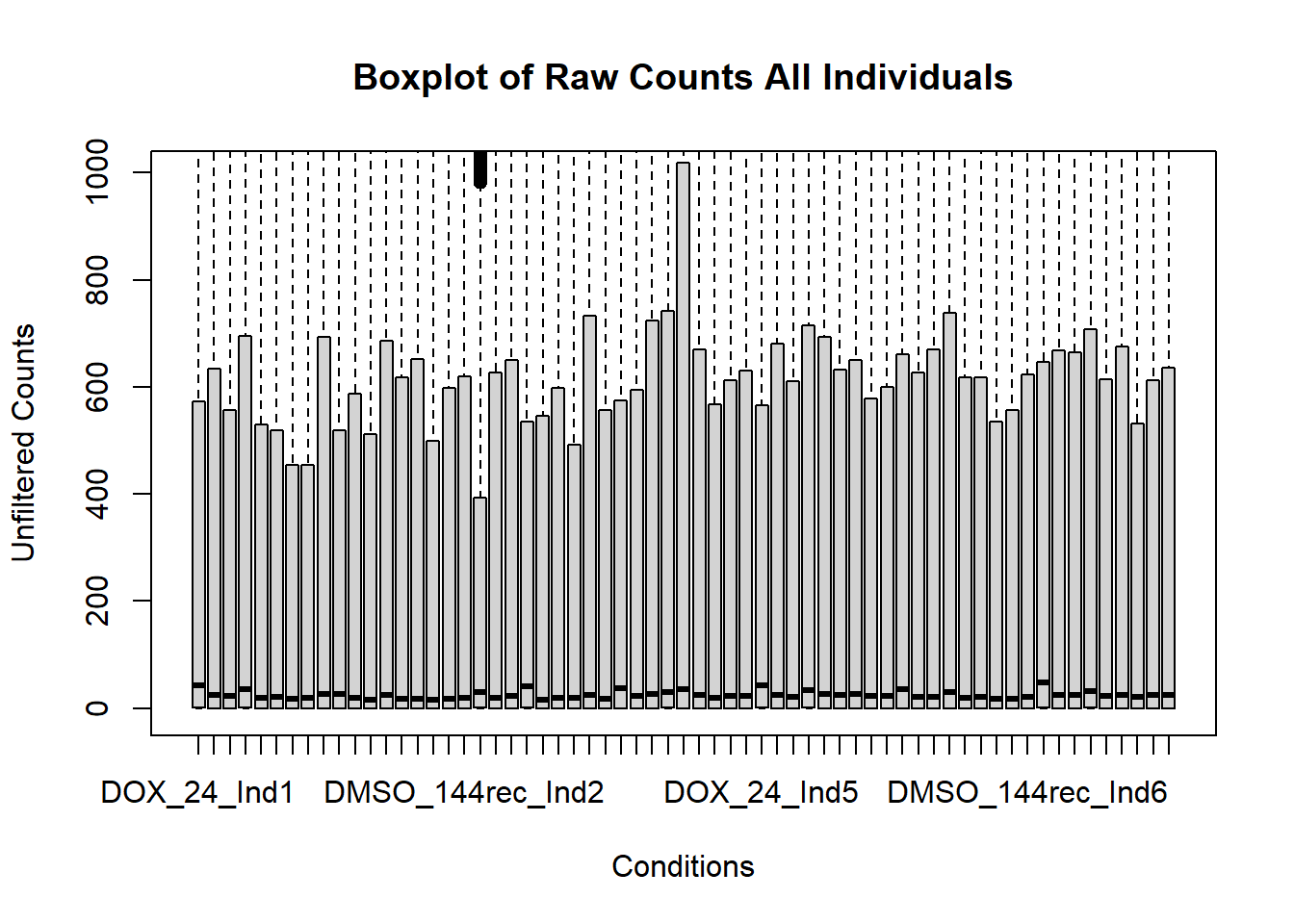
####boxplot log2cpm all samples####

boxplot(fC_Matrix_Full_cpm, xlab = "Conditions", ylab = expression("log"[2]* "counts per million"), ylim= c(-10, 20), main = "Boxplots of log2cpm per sample")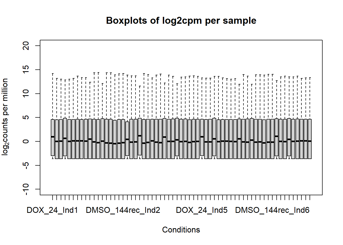
####boxplot log2cpm filtered all samples####

boxplot(fC_Matrix_Full_cpm_filter, xlab = "Conditions", ylab = expression("log"[2]* "counts per million"), ylim= c(-10, 20), main = "Boxplots of log2cpm Filtered rowMeans > 0 per sample")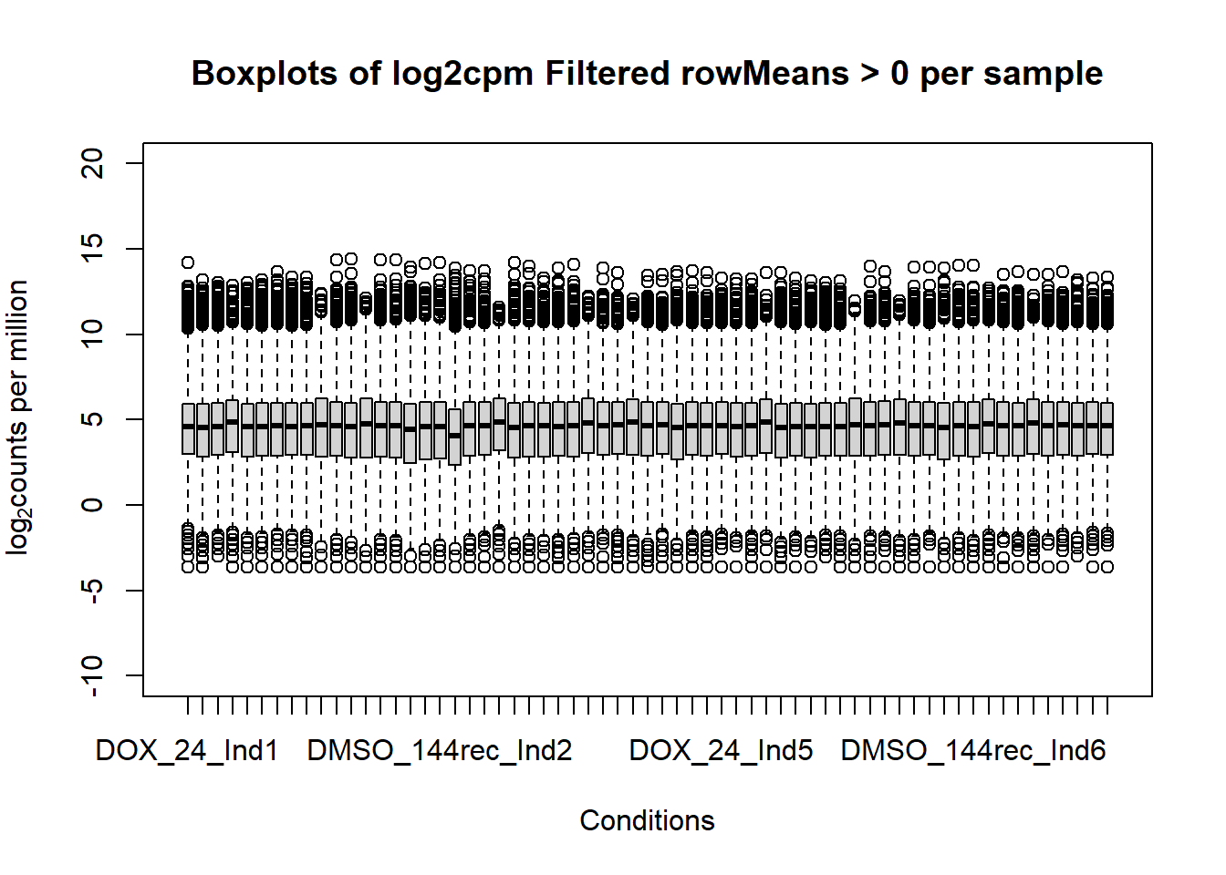
Now that I’ve filtered the samples after log2cpm conversion, I can start to make heatmaps and PCA plots to look at my data
After trying and failing to get all three factors on one PCA plot - I will make iterations of each of these with two factors each
Now, I want to update these PCA plots to have treatment and time as the primary variables Individual will be a fill? Or somehow get some numbers labelled on the points.
PCA_data <- fC_Matrix_Full_cpm_filter %>%
  prcomp(.) %>%
  t()

PCA_data_test <- (prcomp(t(fC_Matrix_Full_cpm_filter), scale. = TRUE))

####now make an annotation for my PCA####
annot <- data.frame("samples" = colnames(fC_Matrix_Full_cpm_filter)) %>% separate_wider_delim(., cols = samples, names = c("Tx", "Time", "Ind"), delim = "_", cols_remove = FALSE) %>% unite(., col = "Tx_Time", Tx, Time, sep = "_", remove = FALSE)

#combine the prcomp matrix and annotation
annot_PCA_matrix <- PCA_data_test$x %>% cbind(., annot)

#now I can make a graph where I have filled values for individual! I have seven colors for seven individuals
# I have three fill values for three timepoints

#using annotation matrix above as well as annotated PCA matrix (annot_PCA_matrix)

#extra info for colors in the graph (fill parameter)
fill_col_ind <- c("#66C2A5", "#FC8D62", "#1F78B4", "#E78AC3", "#A6D854", "#FFD92A", "#8B3E9B")

fill_col_ind_dark <- c("#003F5C", "#45AE91",  "#58508D", "#BC4099", "#8B3E9B", "#FF6361", "#FF2362")

fill_col_tx <- c("#63666D", "#DCACED", "#499FBD")

#Now I have to switch the fill and color parameters as it's doing the opposite of what I wanted: need individuals to be the outline color (color), and tx to be the inside color (fill)

####PC1/PC2####
annot_PCA_matrix %>% ggplot(., aes(x=PC1, y=PC2, size = 10)) +
  geom_point(aes(color = Ind, shape = Time, fill = Tx)) +
                       scale_shape_manual(values = c(21, 22, 24)) +
  scale_fill_manual(values =  fill_col_tx)+
  scale_color_manual(values = c(fill_col_ind_dark))+
  guides(fill=guide_legend(override.aes=list(shape=21)))+
  guides(color=guide_legend(override.aes=list(shape=21)))+
  guides(fill=guide_legend(override.aes=list(shape=21,fill=fill_col_tx,color=fill_col_tx)))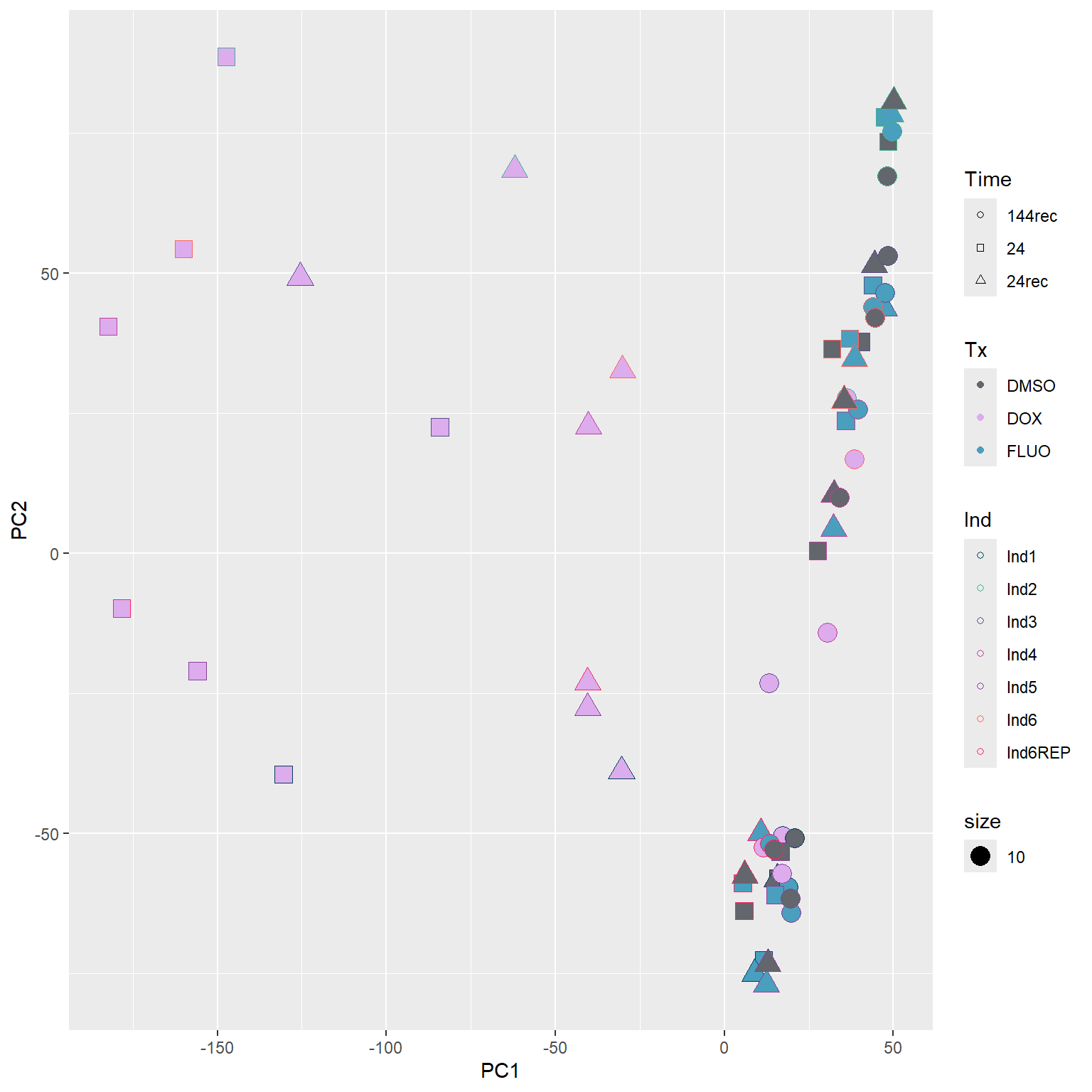
####PC2/PC3####
annot_PCA_matrix %>% ggplot(., aes(x=PC2, y=PC3)) +
  geom_point(aes(color = Ind, shape = Time, fill = Tx, size = 10)) +
                       scale_shape_manual(values = c(21, 22, 24)) +
  scale_fill_manual(values =  fill_col_tx)+
  scale_color_manual(values = c(fill_col_ind_dark))+
  guides(fill=guide_legend(override.aes=list(shape=21)))+
  guides(color=guide_legend(override.aes=list(shape=21)))+
  guides(fill=guide_legend(override.aes=list(shape=21,fill=fill_col_tx,color=fill_col_tx)))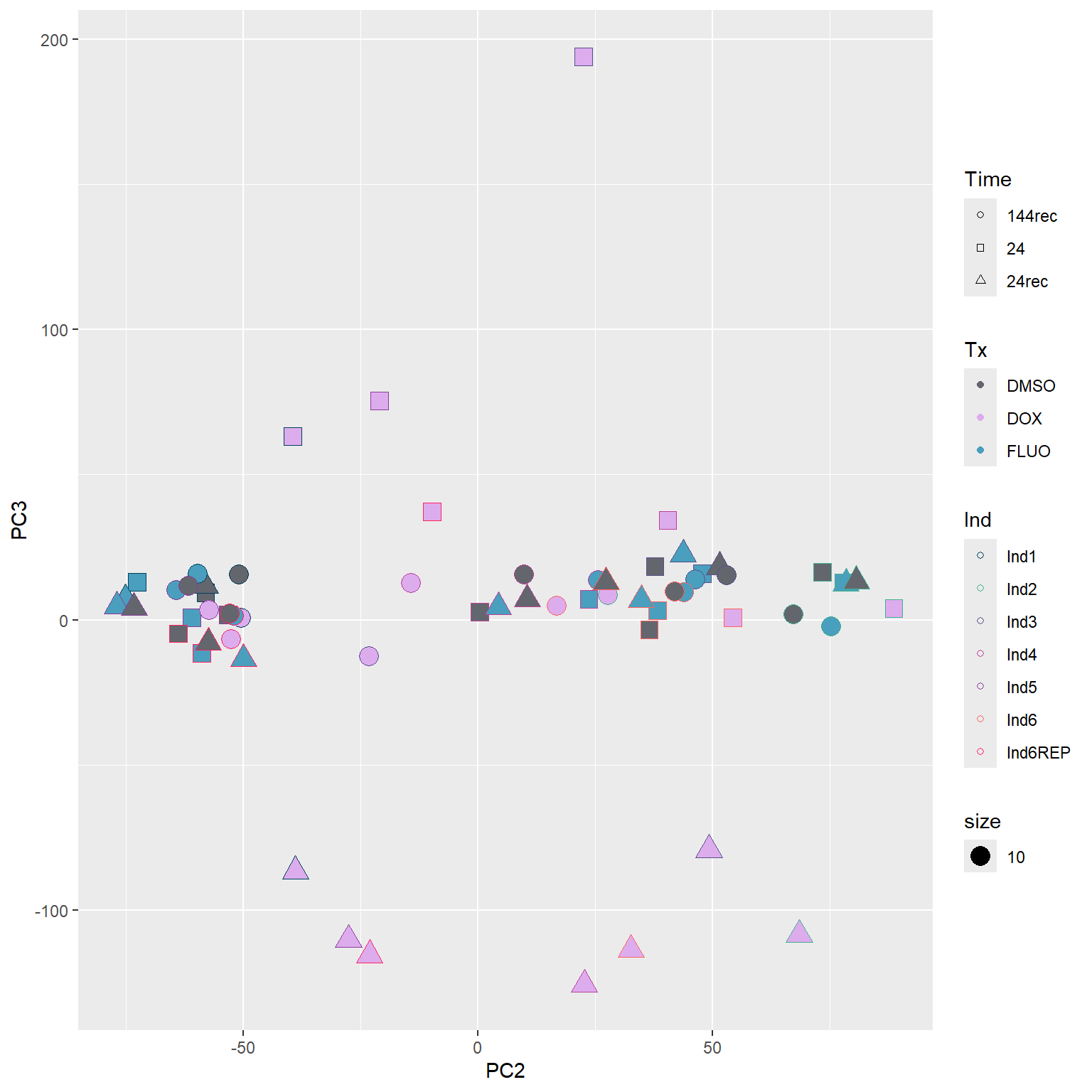
####PC3/PC4####
annot_PCA_matrix %>% ggplot(., aes(x=PC3, y=PC4)) +
  geom_point(aes(color = Ind, shape = Time, fill = Tx, size = 10)) +
                       scale_shape_manual(values = c(21, 22, 24)) +
  scale_fill_manual(values =  fill_col_tx)+
  scale_color_manual(values = c(fill_col_ind_dark))+
  guides(fill=guide_legend(override.aes=list(shape=21)))+
  guides(color=guide_legend(override.aes=list(shape=21)))+
  guides(fill=guide_legend(override.aes=list(shape=21,fill=fill_col_tx,color=fill_col_tx)))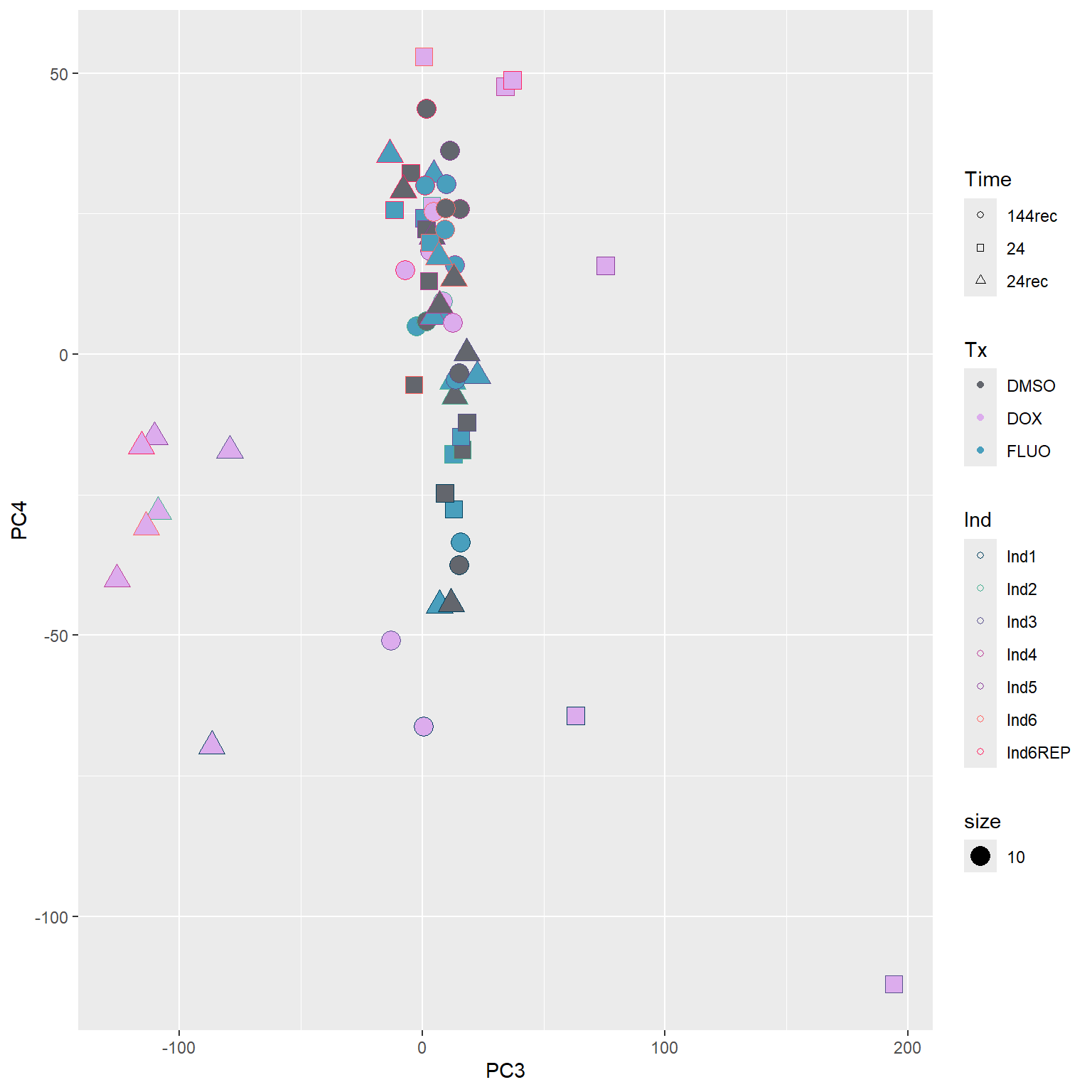
#correlation heatmap for all samples

####PEARSON FILTERED####
fC_Matrix_Full_cpm_filter_pearsoncor <-
  cor(
    fC_Matrix_Full_cpm_filter,
    y = NULL,
    use = "everything",
    method = "pearson"
  )

####SPEARMAN FILTERED####
fC_Matrix_Full_cpm_filter_spearmancor <-
  cor(
    fC_Matrix_Full_cpm_filter,
    y = NULL,
    use = "everything",
    method = "spearman"
  )


#Now let's graph these correlations

pheatmap(fC_Matrix_Full_cpm_filter_pearsoncor, border_color = "black", legend = TRUE, angle_col = 90, display_numbers = FALSE, number_color = "black", fontsize = 12, fontsize_number = 9)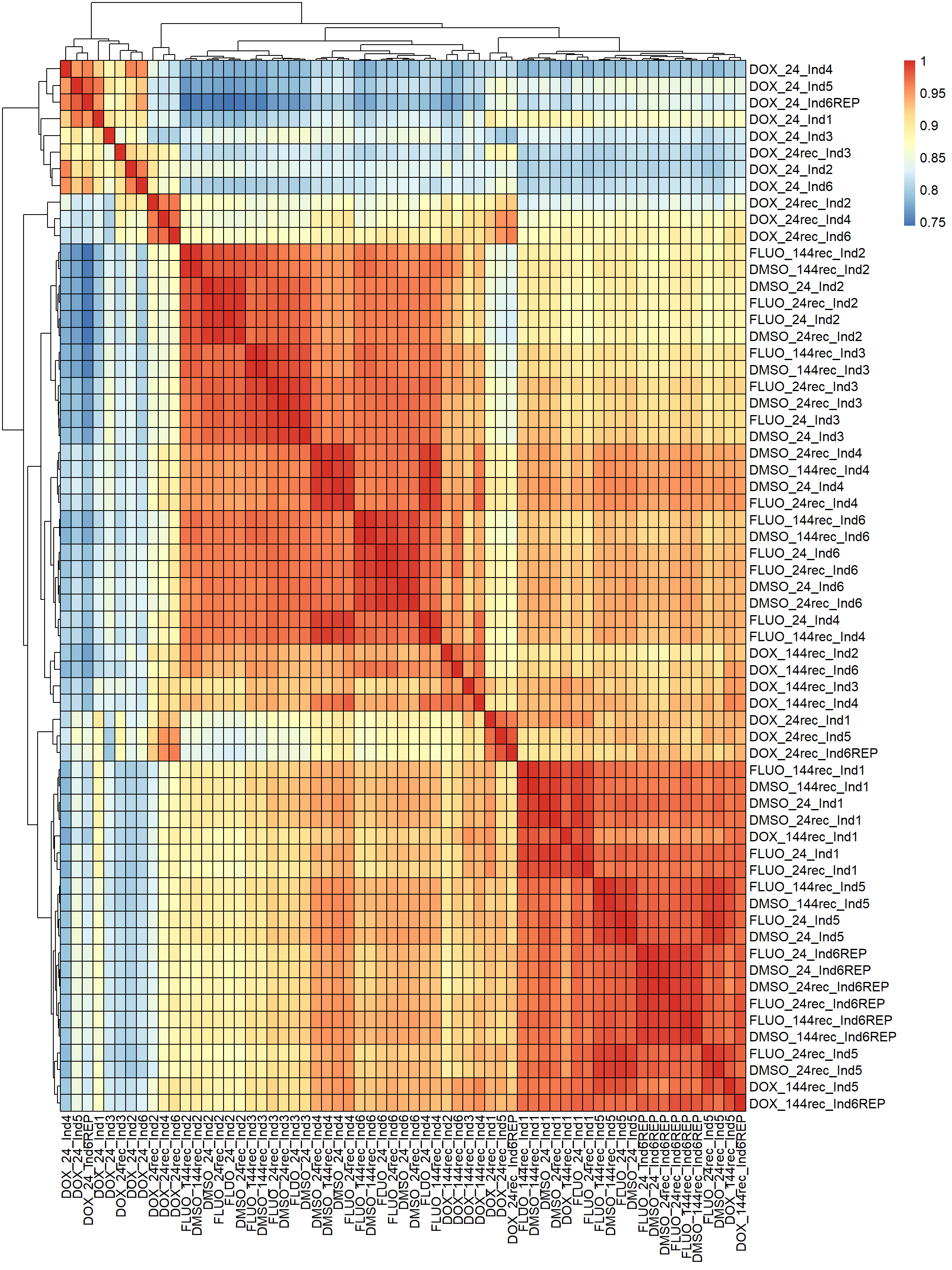
pheatmap(fC_Matrix_Full_cpm_filter_spearmancor, border_color = "black", legend = TRUE, angle_col = 90, display_numbers = FALSE, number_color = "black", fontsize = 12, fontsize_number = 9)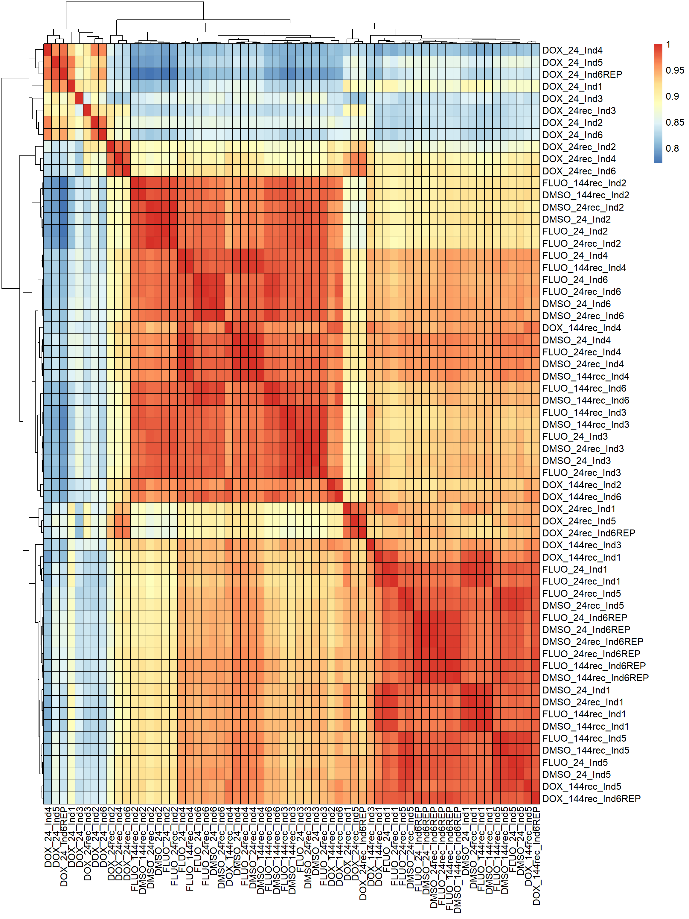
#now annotate these heatmaps
#Factor 1 - Individual
Individual <- as.factor(c(rep("Ind1", 9), rep("Ind2", 9), rep("Ind3", 9), rep("Ind4", 9), rep("Ind5", 9), rep("Ind6", 9), rep("Ind6REP", 9)))

#Factor 2 - Treatment
tx_factor <- c("DOX", "FLUO", "DMSO")
Tx <- as.factor(c(rep(tx_factor, 21)))
#view(Treatment)

#Factor 3 - Timepoint
time_factor <- c(rep("24", 3), rep("24rec", 3), rep("144rec", 3))
Time <- as.factor(c(rep(time_factor, 7)))

####annotation for colors####
annot_col_hm = list(Tx = c(DOX = "red", FLUO = "blue", DMSO = "black"),
                             Ind = c(Ind1 = "#66C2A5", Ind2 = "#FC8D62", Ind3 = "#1F78B4", Ind4 = "#E78AC3", Ind5 = "#A6D854", Ind6 = "#FFD92A", Ind6REP = "#8B3E9B"),
                             Time = c("24" = "#046A38", "24rec" = "#0050B5", "144rec" = "#B725AD"))

####annotation for values####
annot_list_hm <- data.frame(Individual = as.factor(c(rep("Ind1", 9), rep("Ind2", 9), rep("Ind3", 9), rep("Ind4", 9), rep("Ind5", 9), rep("Ind6", 9), rep("Ind6REP", 9))),
                                               Tx = as.factor(c(rep(tx_factor, 21))),
                                               Time = as.factor(c(rep(time_factor, 7))))


##add in the annotations from above into the dataframe
row.names(annot_list_hm) <- colnames(fC_Matrix_Full_cpm_filter_pearsoncor)
row.names(annot_list_hm) <- colnames(fC_Matrix_Full_cpm_filter_spearmancor)

####ANNOTATED HEATMAPS####
pheatmap(fC_Matrix_Full_cpm_filter_pearsoncor, border_color = "black", legend = TRUE, angle_col = 90, display_numbers = FALSE, number_color = "black", fontsize = 10, fontsize_number = 5, annotation_col = annot_list_hm, annotation_colors = annot_col_hm)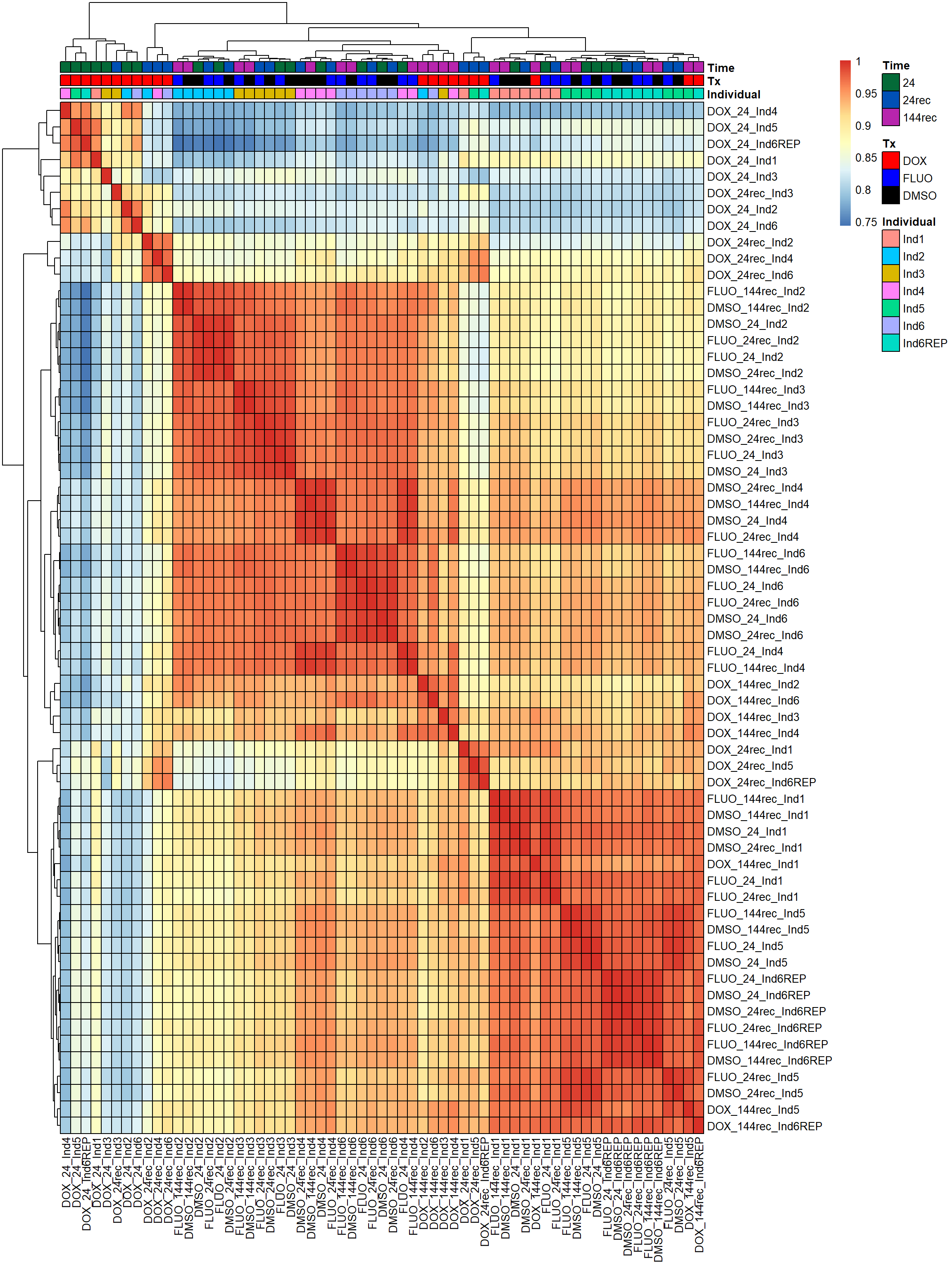
pheatmap(fC_Matrix_Full_cpm_filter_spearmancor, border_color = "black", legend = TRUE, angle_col = 90, display_numbers = FALSE, number_color = "black", fontsize = 10, fontsize_number = 5, annotation_col = annot_list_hm, annotation_colors = annot_col_hm)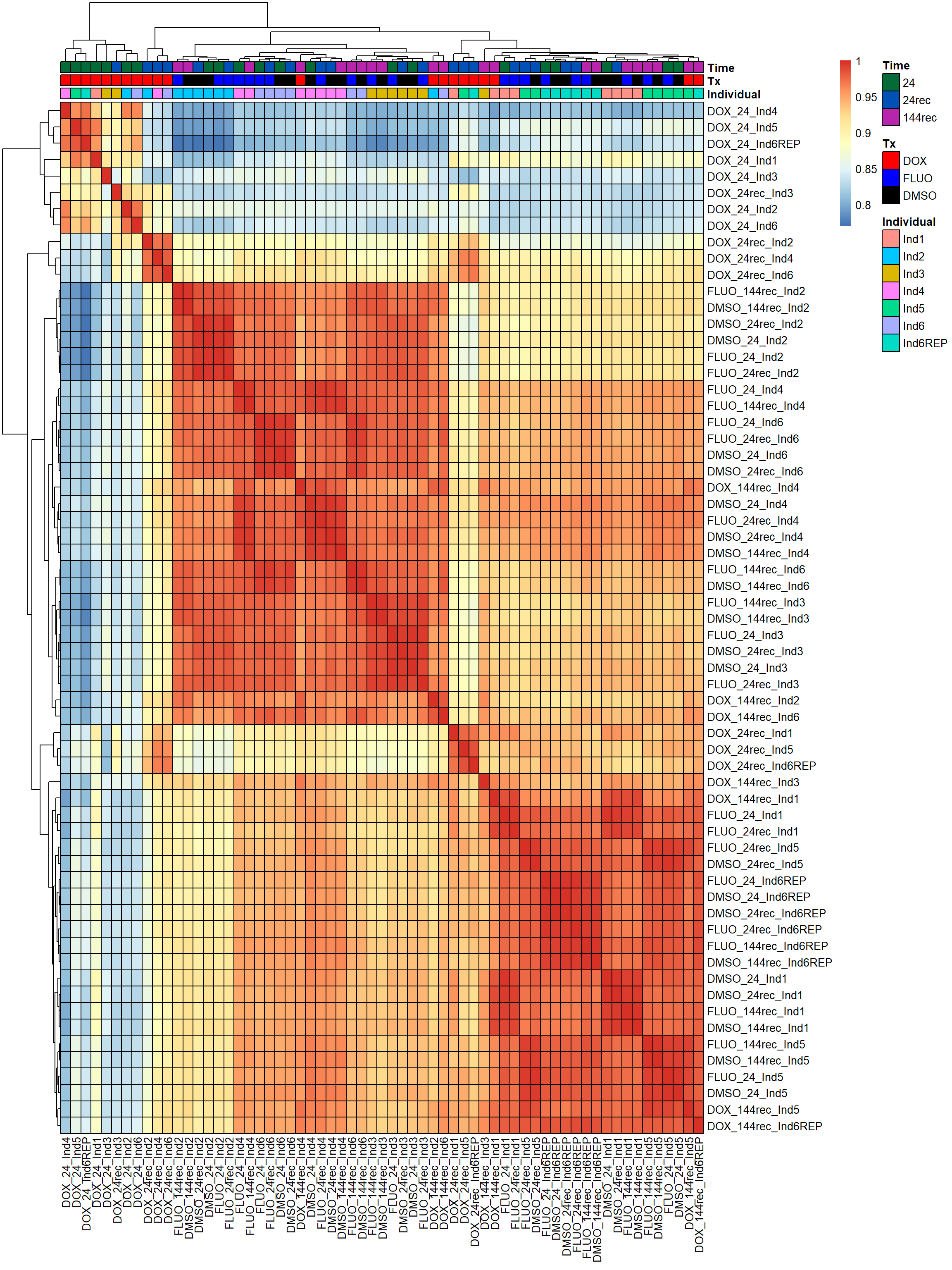
# group <- c(rep(c(1, 2, 3, 4, 5, 6, 7, 8, 9), 6))
# group <- factor(group, levels = c("1", "2", "3", "4", "5", "6", "7", "8", "9"))


####rowMeans > 0 Filtering####
rowMeans_DE <- rowMeans(counts_DE)
counts_DE_filter <- counts_DE[rowMeans_DE > 0,]
dim(counts_DE_filter)
[1] 26445    54

group_1 <- rep(c("DOX_24","FLUO_24",
                                "DMSO_24",
                                "DOX_24rec",
                                "FLUO_24rec",
                                "DMSO_24rec",
                                "DOX_144rec",
                                "FLUO_144rec",
                                "DMSO_144rec"), 6)

dge <- DGEList.data.frame(counts = counts_DE_filter, group = group_1, genes = row.names(counts_DE_filter))

#this is the inital file before norm factors are calculated
dge$samples
                       group lib.size norm.factors
DOX_24_Ind1           DOX_24 23533985            1
FLUO_24_Ind1         FLUO_24 26970695            1
DMSO_24_Ind1         DMSO_24 22892686            1
DOX_24rec_Ind1     DOX_24rec 23932153            1
FLUO_24rec_Ind1   FLUO_24rec 21879931            1
DMSO_24rec_Ind1   DMSO_24rec 21337454            1
DOX_144rec_Ind1   DOX_144rec 18260440            1
FLUO_144rec_Ind1 FLUO_144rec 18780865            1
DMSO_144rec_Ind1 DMSO_144rec 28167799            1
DOX_24_Ind2           DOX_24 20017534            1
FLUO_24_Ind2         FLUO_24 23930827            1
DMSO_24_Ind2         DMSO_24 21334270            1
DOX_24rec_Ind2     DOX_24rec 25714988            1
FLUO_24rec_Ind2   FLUO_24rec 25160237            1
DMSO_24rec_Ind2   DMSO_24rec 26356290            1
DOX_144rec_Ind2   DOX_144rec 23497279            1
FLUO_144rec_Ind2 FLUO_144rec 24769290            1
DMSO_144rec_Ind2 DMSO_144rec 25878841            1
DOX_24_Ind3           DOX_24 23195184            1
FLUO_24_Ind3         FLUO_24 25146622            1
DMSO_24_Ind3         DMSO_24 25648723            1
DOX_24rec_Ind3     DOX_24rec 18250610            1
FLUO_24rec_Ind3   FLUO_24rec 23122465            1
DMSO_24rec_Ind3   DMSO_24rec 24364234            1
DOX_144rec_Ind3   DOX_144rec 19801072            1
FLUO_144rec_Ind3 FLUO_144rec 29845161            1
DMSO_144rec_Ind3 DMSO_144rec 22672688            1
DOX_24_Ind4           DOX_24 20726954            1
FLUO_24_Ind4         FLUO_24 23704697            1
DMSO_24_Ind4         DMSO_24 28213836            1
DOX_24rec_Ind4     DOX_24rec 25911782            1
FLUO_24rec_Ind4   FLUO_24rec 40622129            1
DMSO_24rec_Ind4   DMSO_24rec 26124863            1
DOX_144rec_Ind4   DOX_144rec 24701727            1
FLUO_144rec_Ind4 FLUO_144rec 24610641            1
DMSO_144rec_Ind4 DMSO_144rec 25455999            1
DOX_24_Ind5           DOX_24 22697304            1
FLUO_24_Ind5         FLUO_24 27856508            1
DMSO_24_Ind5         DMSO_24 24639151            1
DOX_24rec_Ind5     DOX_24rec 24885980            1
FLUO_24rec_Ind5   FLUO_24rec 29665028            1
DMSO_24rec_Ind5   DMSO_24rec 26036618            1
DOX_144rec_Ind5   DOX_144rec 27513167            1
FLUO_144rec_Ind5 FLUO_144rec 23993986            1
DMSO_144rec_Ind5 DMSO_144rec 24942365            1
DOX_24_Ind6           DOX_24 25308109            1
FLUO_24_Ind6         FLUO_24 25269296            1
DMSO_24_Ind6         DMSO_24 25666994            1
DOX_24rec_Ind6     DOX_24rec 26209951            1
FLUO_24rec_Ind6   FLUO_24rec 25079566            1
DMSO_24rec_Ind6   DMSO_24rec 24465515            1
DOX_144rec_Ind6   DOX_144rec 23359517            1
FLUO_144rec_Ind6 FLUO_144rec 22471386            1
DMSO_144rec_Ind6 DMSO_144rec 25460267            1

#calculate the normalization factors with method TMM
dge_calc <- calcNormFactors(dge, method = "TMM")

#final file after norm calculation
dge_calc$samples
                       group lib.size norm.factors
DOX_24_Ind1           DOX_24 23533985    1.0837997
FLUO_24_Ind1         FLUO_24 26970695    0.9310699
DMSO_24_Ind1         DMSO_24 22892686    0.9611153
DOX_24rec_Ind1     DOX_24rec 23932153    1.2332319
FLUO_24rec_Ind1   FLUO_24rec 21879931    0.9480185
DMSO_24rec_Ind1   DMSO_24rec 21337454    0.9725610
DOX_144rec_Ind1   DOX_144rec 18260440    1.0159884
FLUO_144rec_Ind1 FLUO_144rec 18780865    0.9797092
DMSO_144rec_Ind1 DMSO_144rec 28167799    0.9690593
DOX_24_Ind2           DOX_24 20017534    1.1031490
FLUO_24_Ind2         FLUO_24 23930827    0.9960906
DMSO_24_Ind2         DMSO_24 21334270    0.9579222
DOX_24rec_Ind2     DOX_24rec 25714988    1.0897455
FLUO_24rec_Ind2   FLUO_24rec 25160237    0.9709110
DMSO_24rec_Ind2   DMSO_24rec 26356290    0.9632263
DOX_144rec_Ind2   DOX_144rec 23497279    0.8853001
FLUO_144rec_Ind2 FLUO_144rec 24769290    0.9818596
DMSO_144rec_Ind2 DMSO_144rec 25878841    0.9747532
DOX_24_Ind3           DOX_24 23195184    0.8512838
FLUO_24_Ind3         FLUO_24 25146622    0.9755381
DMSO_24_Ind3         DMSO_24 25648723    0.9934558
DOX_24rec_Ind3     DOX_24rec 18250610    1.3034379
FLUO_24rec_Ind3   FLUO_24rec 23122465    0.9351582
DMSO_24rec_Ind3   DMSO_24rec 24364234    0.9693937
DOX_144rec_Ind3   DOX_144rec 19801072    1.0246641
FLUO_144rec_Ind3 FLUO_144rec 29845161    0.9803051
DMSO_144rec_Ind3 DMSO_144rec 22672688    0.9806025
DOX_24_Ind4           DOX_24 20726954    1.1649074
FLUO_24_Ind4         FLUO_24 23704697    0.9849905
DMSO_24_Ind4         DMSO_24 28213836    0.9912683
DOX_24rec_Ind4     DOX_24rec 25911782    1.1791631
FLUO_24rec_Ind4   FLUO_24rec 40622129    0.9751981
DMSO_24rec_Ind4   DMSO_24rec 26124863    0.9981792
DOX_144rec_Ind4   DOX_144rec 24701727    0.9176890
FLUO_144rec_Ind4 FLUO_144rec 24610641    0.9816716
DMSO_144rec_Ind4 DMSO_144rec 25455999    0.9636547
DOX_24_Ind5           DOX_24 22697304    1.0773544
FLUO_24_Ind5         FLUO_24 27856508    0.9397778
DMSO_24_Ind5         DMSO_24 24639151    0.9538894
DOX_24rec_Ind5     DOX_24rec 24885980    1.2233210
FLUO_24rec_Ind5   FLUO_24rec 29665028    0.9193648
DMSO_24rec_Ind5   DMSO_24rec 26036618    0.9527365
DOX_144rec_Ind5   DOX_144rec 27513167    0.9469333
FLUO_144rec_Ind5 FLUO_144rec 23993986    0.9381287
DMSO_144rec_Ind5 DMSO_144rec 24942365    0.9285333
DOX_24_Ind6           DOX_24 25308109    1.0981454
FLUO_24_Ind6         FLUO_24 25269296    0.9948090
DMSO_24_Ind6         DMSO_24 25666994    1.0159532
DOX_24rec_Ind6     DOX_24rec 26209951    1.1400925
FLUO_24rec_Ind6   FLUO_24rec 25079566    0.9794435
DMSO_24rec_Ind6   DMSO_24rec 24465515    0.9860363
DOX_144rec_Ind6   DOX_144rec 23359517    0.9397642
FLUO_144rec_Ind6 FLUO_144rec 22471386    0.9892227
DMSO_144rec_Ind6 DMSO_144rec 25460267    0.9800208

#View(dge_calc)

#Pull out factors
snames <- data.frame("samples" = colnames(dge_calc)) %>% separate_wider_delim(., cols = samples, names = c("Treatment", "Time", "Individual"), delim = "_", cols_remove = FALSE)

#snames_list <- as.list(snames)

snames_time <- snames$Time
snames_tx <- snames$Treatment
snames_ind <- snames$Individual

#Create my model matrix
mm_r <- model.matrix(~0 + group_1)

p <- voom(dge_calc$counts, mm_r, plot = TRUE)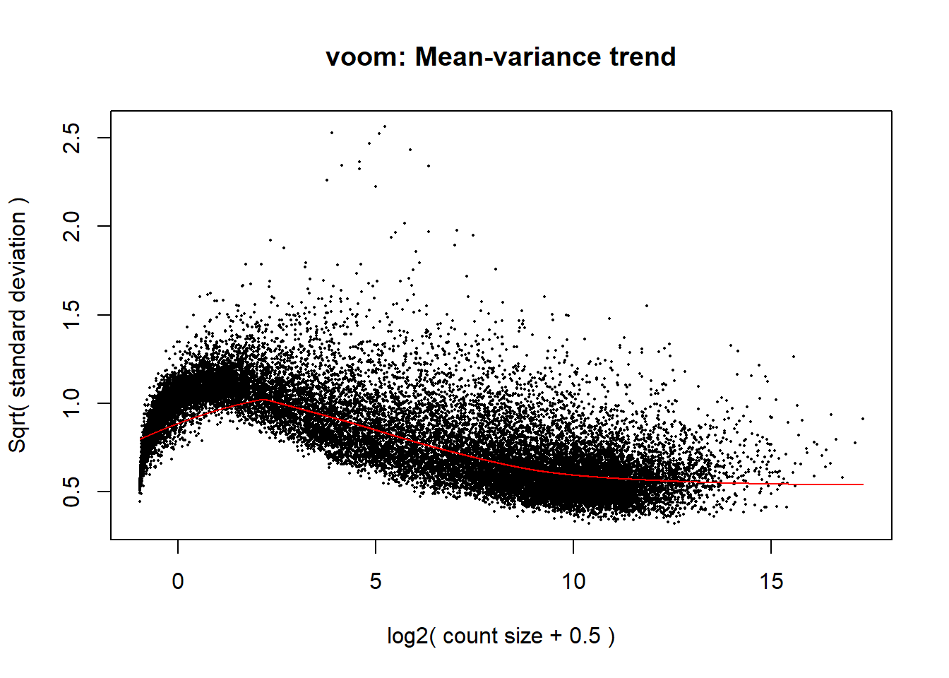
corfit <- duplicateCorrelation(p, mm_r, block = snames_ind)

v <- voom(dge_calc$counts, mm_r, block = snames_ind, correlation = corfit$consensus)

fit <- lmFit(v, mm_r, block = snames_ind, correlation = corfit$consensus)

#make sure to check which order the columns are in - otherwise they won't match right (it was moved into alphabetical and number order)
colnames(mm_r) <- c("DMSO_144rec","DMSO_24","DMSO_24rec","DOX_144rec","DOX_24","DOX_24rec","FLUO_144rec","FLUO_24","FLUO_24rec")

cm_r <- makeContrasts(
        V.D24 = DOX_24 - DMSO_24,
        V.F24 = FLUO_24 - DMSO_24,
        V.D24r = DOX_24rec - DMSO_24rec,
        V.F24r = FLUO_24rec - DMSO_24rec,
        V.D144r = DOX_144rec - DMSO_144rec,
        V.F144r = FLUO_144rec - DMSO_144rec,
        levels = mm_r
)

vfit_r <- lmFit(p, mm_r)
vfit_r <- contrasts.fit(vfit_r, contrasts = cm_r)

efit2 <- eBayes(vfit_r)

results = decideTests(efit2)
summary(results)
       V.D24 V.F24 V.D24r V.F24r V.D144r V.F144r
Down    4567     0   2083      0     288       0
NotSig 14521 26445  16339  26445   25296   26445
Up      7357     0   8023      0     861       0
#inbuilt annotation results rowMeans >0
#         V.D24 V.F24 V.D24r V.F24r V.D144r V.F144r
# Down    4567     0   2083      0     288       0
# NotSig 14521 26445  16339  26445   25296   26445
# Up      7357     0   8023      0     861       0

## have no DE genes detected for 5FU, only DOX


####plot your voom####
voom_plot <- voom(dge_calc, mm_r, plot = TRUE)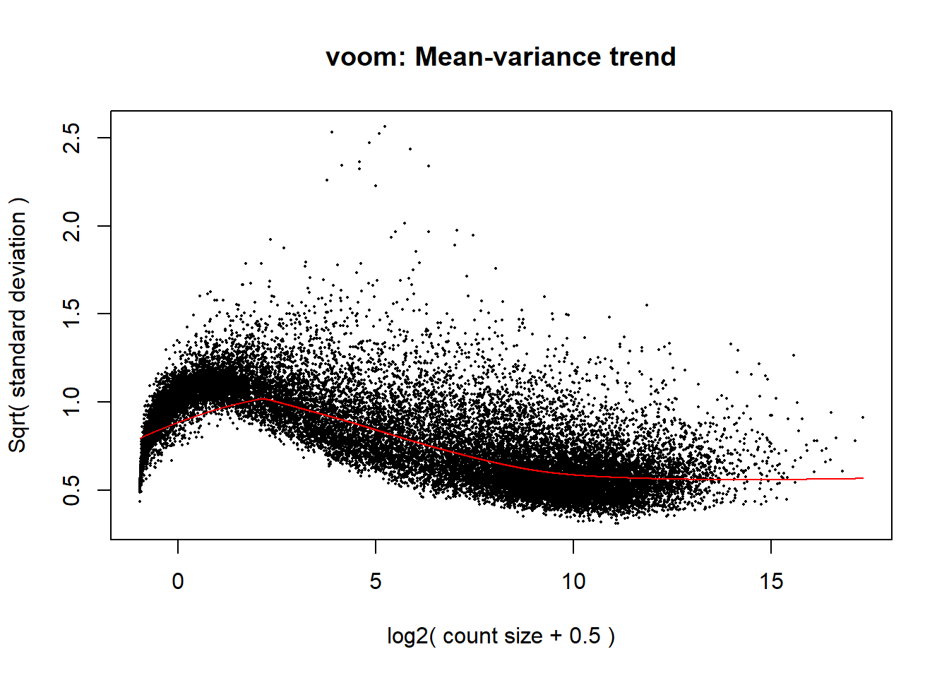
The voom plot for this with rowMeans > 0 has a dip in the front, meaning that there is likely some noise left over in my data. I am going to filter a bit stricter at rowMeans > 1 with the same process as above.
####rowMeans >1####
rowMeans_DE <- rowMeans(counts_DE)
counts_DE_filter1 <- counts_DE[rowMeans_DE > 1,]
dim(counts_DE_filter1)
[1] 20443    54


dge1 <- DGEList.data.frame(counts = counts_DE_filter1, group = group_1, genes = row.names(counts_DE_filter1))

#this is the inital file before norm factors are calculated
dge1$samples
                       group lib.size norm.factors
DOX_24_Ind1           DOX_24 23529436            1
FLUO_24_Ind1         FLUO_24 26969621            1
DMSO_24_Ind1         DMSO_24 22891830            1
DOX_24rec_Ind1     DOX_24rec 23928177            1
FLUO_24rec_Ind1   FLUO_24rec 21879021            1
DMSO_24rec_Ind1   DMSO_24rec 21336552            1
DOX_144rec_Ind1   DOX_144rec 18258678            1
FLUO_144rec_Ind1 FLUO_144rec 18779997            1
DMSO_144rec_Ind1 DMSO_144rec 28166609            1
DOX_24_Ind2           DOX_24 20015891            1
FLUO_24_Ind2         FLUO_24 23929971            1
DMSO_24_Ind2         DMSO_24 21333555            1
DOX_24rec_Ind2     DOX_24rec 25712271            1
FLUO_24rec_Ind2   FLUO_24rec 25159540            1
DMSO_24rec_Ind2   DMSO_24rec 26355579            1
DOX_144rec_Ind2   DOX_144rec 23495279            1
FLUO_144rec_Ind2 FLUO_144rec 24768504            1
DMSO_144rec_Ind2 DMSO_144rec 25877847            1
DOX_24_Ind3           DOX_24 23190452            1
FLUO_24_Ind3         FLUO_24 25145882            1
DMSO_24_Ind3         DMSO_24 25647796            1
DOX_24rec_Ind3     DOX_24rec 18243178            1
FLUO_24rec_Ind3   FLUO_24rec 23121928            1
DMSO_24rec_Ind3   DMSO_24rec 24363550            1
DOX_144rec_Ind3   DOX_144rec 19797829            1
FLUO_144rec_Ind3 FLUO_144rec 29844009            1
DMSO_144rec_Ind3 DMSO_144rec 22672047            1
DOX_24_Ind4           DOX_24 20724269            1
FLUO_24_Ind4         FLUO_24 23703826            1
DMSO_24_Ind4         DMSO_24 28212829            1
DOX_24rec_Ind4     DOX_24rec 25908531            1
FLUO_24rec_Ind4   FLUO_24rec 40620908            1
DMSO_24rec_Ind4   DMSO_24rec 26124015            1
DOX_144rec_Ind4   DOX_144rec 24699442            1
FLUO_144rec_Ind4 FLUO_144rec 24609834            1
DMSO_144rec_Ind4 DMSO_144rec 25455151            1
DOX_24_Ind5           DOX_24 22693201            1
FLUO_24_Ind5         FLUO_24 27855535            1
DMSO_24_Ind5         DMSO_24 24638257            1
DOX_24rec_Ind5     DOX_24rec 24881937            1
FLUO_24rec_Ind5   FLUO_24rec 29663662            1
DMSO_24rec_Ind5   DMSO_24rec 26035482            1
DOX_144rec_Ind5   DOX_144rec 27510410            1
FLUO_144rec_Ind5 FLUO_144rec 23992921            1
DMSO_144rec_Ind5 DMSO_144rec 24941416            1
DOX_24_Ind6           DOX_24 25305699            1
FLUO_24_Ind6         FLUO_24 25268538            1
DMSO_24_Ind6         DMSO_24 25666263            1
DOX_24rec_Ind6     DOX_24rec 26207393            1
FLUO_24rec_Ind6   FLUO_24rec 25078845            1
DMSO_24rec_Ind6   DMSO_24rec 24464720            1
DOX_144rec_Ind6   DOX_144rec 23357605            1
FLUO_144rec_Ind6 FLUO_144rec 22470700            1
DMSO_144rec_Ind6 DMSO_144rec 25459487            1

#calculate the normalization factors with method TMM
dge1_calc <- calcNormFactors(dge1, method = "TMM")

#final file after norm calculation
dge1_calc$samples
                       group lib.size norm.factors
DOX_24_Ind1           DOX_24 23529436    1.1010478
FLUO_24_Ind1         FLUO_24 26969621    0.9224026
DMSO_24_Ind1         DMSO_24 22891830    0.9523318
DOX_24rec_Ind1     DOX_24rec 23928177    1.2419707
FLUO_24rec_Ind1   FLUO_24rec 21879021    0.9414647
DMSO_24rec_Ind1   DMSO_24rec 21336552    0.9714352
DOX_144rec_Ind1   DOX_144rec 18258678    1.0061282
FLUO_144rec_Ind1 FLUO_144rec 18779997    0.9577701
DMSO_144rec_Ind1 DMSO_144rec 28166609    0.9633660
DOX_24_Ind2           DOX_24 20015891    1.1311547
FLUO_24_Ind2         FLUO_24 23929971    1.0037288
DMSO_24_Ind2         DMSO_24 21333555    0.9711101
DOX_24rec_Ind2     DOX_24rec 25712271    1.0919406
FLUO_24rec_Ind2   FLUO_24rec 25159540    0.9757042
DMSO_24rec_Ind2   DMSO_24rec 26355579    0.9694902
DOX_144rec_Ind2   DOX_144rec 23495279    0.8831165
FLUO_144rec_Ind2 FLUO_144rec 24768504    0.9802117
DMSO_144rec_Ind2 DMSO_144rec 25877847    0.9735050
DOX_24_Ind3           DOX_24 23190452    0.8944444
FLUO_24_Ind3         FLUO_24 25145882    0.9787822
DMSO_24_Ind3         DMSO_24 25647796    0.9998010
DOX_24rec_Ind3     DOX_24rec 18243178    1.3366353
FLUO_24rec_Ind3   FLUO_24rec 23121928    0.9387564
DMSO_24rec_Ind3   DMSO_24rec 24363550    0.9645367
DOX_144rec_Ind3   DOX_144rec 19797829    1.0329079
FLUO_144rec_Ind3 FLUO_144rec 29844009    0.9794210
DMSO_144rec_Ind3 DMSO_144rec 22672047    0.9717442
DOX_24_Ind4           DOX_24 20724269    1.2119035
FLUO_24_Ind4         FLUO_24 23703826    0.9874501
DMSO_24_Ind4         DMSO_24 28212829    0.9971983
DOX_24rec_Ind4     DOX_24rec 25908531    1.1839389
FLUO_24rec_Ind4   FLUO_24rec 40620908    0.9545701
DMSO_24rec_Ind4   DMSO_24rec 26124015    0.9903031
DOX_144rec_Ind4   DOX_144rec 24699442    0.9135958
FLUO_144rec_Ind4 FLUO_144rec 24609834    0.9800993
DMSO_144rec_Ind4 DMSO_144rec 25455151    0.9499049
DOX_24_Ind5           DOX_24 22693201    1.1040571
FLUO_24_Ind5         FLUO_24 27855535    0.9171950
DMSO_24_Ind5         DMSO_24 24638257    0.9316924
DOX_24rec_Ind5     DOX_24rec 24881937    1.2117783
FLUO_24rec_Ind5   FLUO_24rec 29663662    0.8980900
DMSO_24rec_Ind5   DMSO_24rec 26035482    0.9397879
DOX_144rec_Ind5   DOX_144rec 27510410    0.9273815
FLUO_144rec_Ind5 FLUO_144rec 23992921    0.9249558
DMSO_144rec_Ind5 DMSO_144rec 24941416    0.9177884
DOX_24_Ind6           DOX_24 25305699    1.1312672
FLUO_24_Ind6         FLUO_24 25268538    0.9892086
DMSO_24_Ind6         DMSO_24 25666263    1.0174650
DOX_24rec_Ind6     DOX_24rec 26207393    1.1422058
FLUO_24rec_Ind6   FLUO_24rec 25078845    0.9747427
DMSO_24rec_Ind6   DMSO_24rec 24464720    0.9836358
DOX_144rec_Ind6   DOX_144rec 23357605    0.9424696
FLUO_144rec_Ind6 FLUO_144rec 22470700    0.9862254
DMSO_144rec_Ind6 DMSO_144rec 25459487    0.9808584

#View(dge1_calc)

#Pull out factors
snames1 <- data.frame("samples" = colnames(dge1_calc)) %>% separate_wider_delim(., cols = samples, names = c("Treatment", "Time", "Individual"), delim = "_", cols_remove = FALSE)

#snames_list <- as.list(snames)

snames1_time <- snames1$Time
snames1_tx <- snames1$Treatment
snames1_ind <- snames1$Individual

#Create my model matrix
mm_r1 <- model.matrix(~0 + group_1)

p1 <- voom(dge1_calc$counts, mm_r1, plot = TRUE)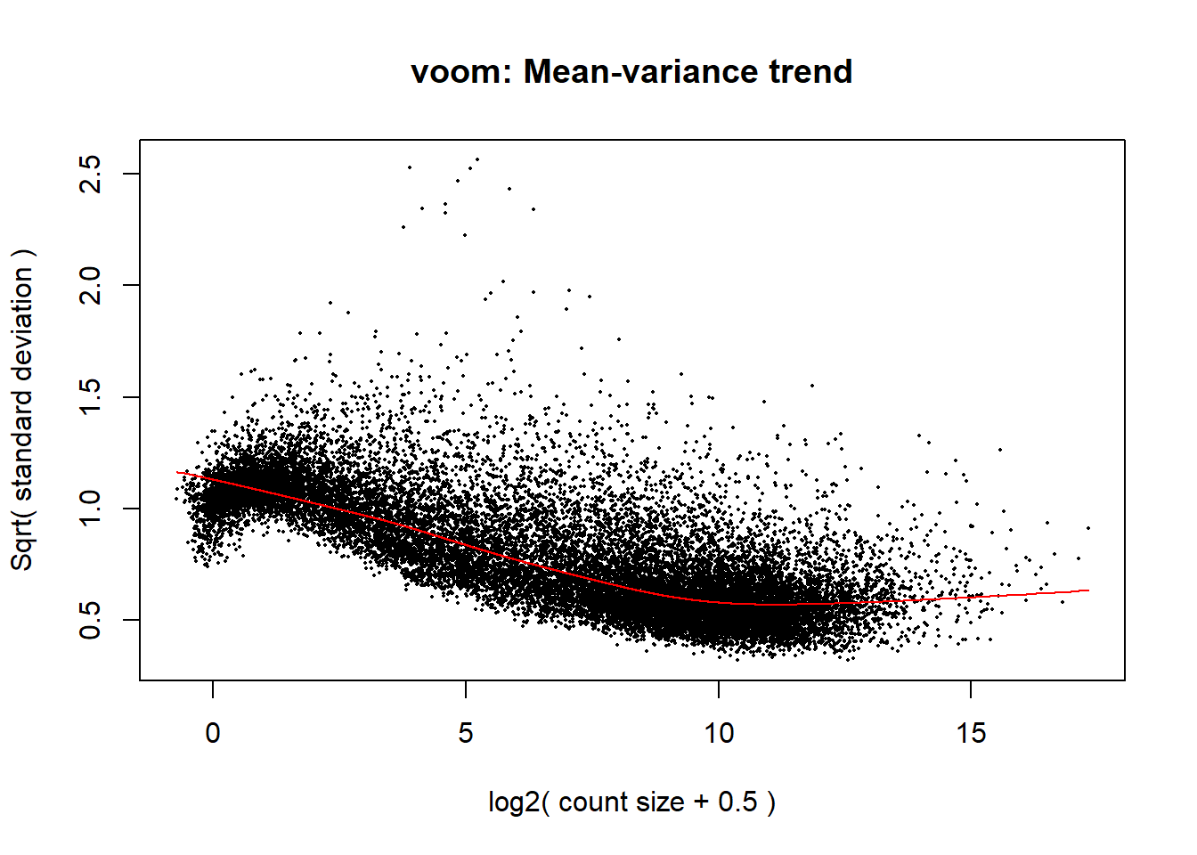
corfit1 <- duplicateCorrelation(p1, mm_r1, block = snames1_ind)
v1 <- voom(dge1_calc$counts, mm_r1, block = snames1_ind, correlation = corfit1$consensus)
fit1 <- lmFit(v1, mm_r1, block = snames1_ind, correlation = corfit1$consensus)
#make sure to check which order the columns are in - otherwise they won't match right (it was moved into alphabetical and number order)
colnames(mm_r1) <- c("DMSO_144rec","DMSO_24","DMSO_24rec","DOX_144rec","DOX_24","DOX_24rec","FLUO_144rec","FLUO_24","FLUO_24rec")
cm_r1 <- makeContrasts(
V.D24 = DOX_24 - DMSO_24,
V.F24 = FLUO_24 - DMSO_24,
V.D24r = DOX_24rec - DMSO_24rec,
V.F24r = FLUO_24rec - DMSO_24rec,
V.D144r = DOX_144rec - DMSO_144rec,
V.F144r = FLUO_144rec - DMSO_144rec,
levels = mm_r1
)
vfit_r1 <- lmFit(p1, mm_r1)
vfit_r1 <- contrasts.fit(vfit_r1, contrasts = cm_r1)
efit4 <- eBayes(vfit_r1)
results1 = decideTests(efit4)
summary(results1)
V.D24 V.F24 V.D24r V.F24r V.D144r V.F144r
Down 4640 0 2120 0 263 0
NotSig 9460 20443 11485 20443 19838 20443
Up 6343 0 6838 0 342 0
#inbuilt annotation results rowMeans >0
# V.D24 V.F24 V.D24r V.F24r V.D144r V.F144r
# Down 4567 0 2083 0 288 0
# NotSig 14521 26445 16339 26445 25296 26445
# Up 7357 0 8023 0 861 0
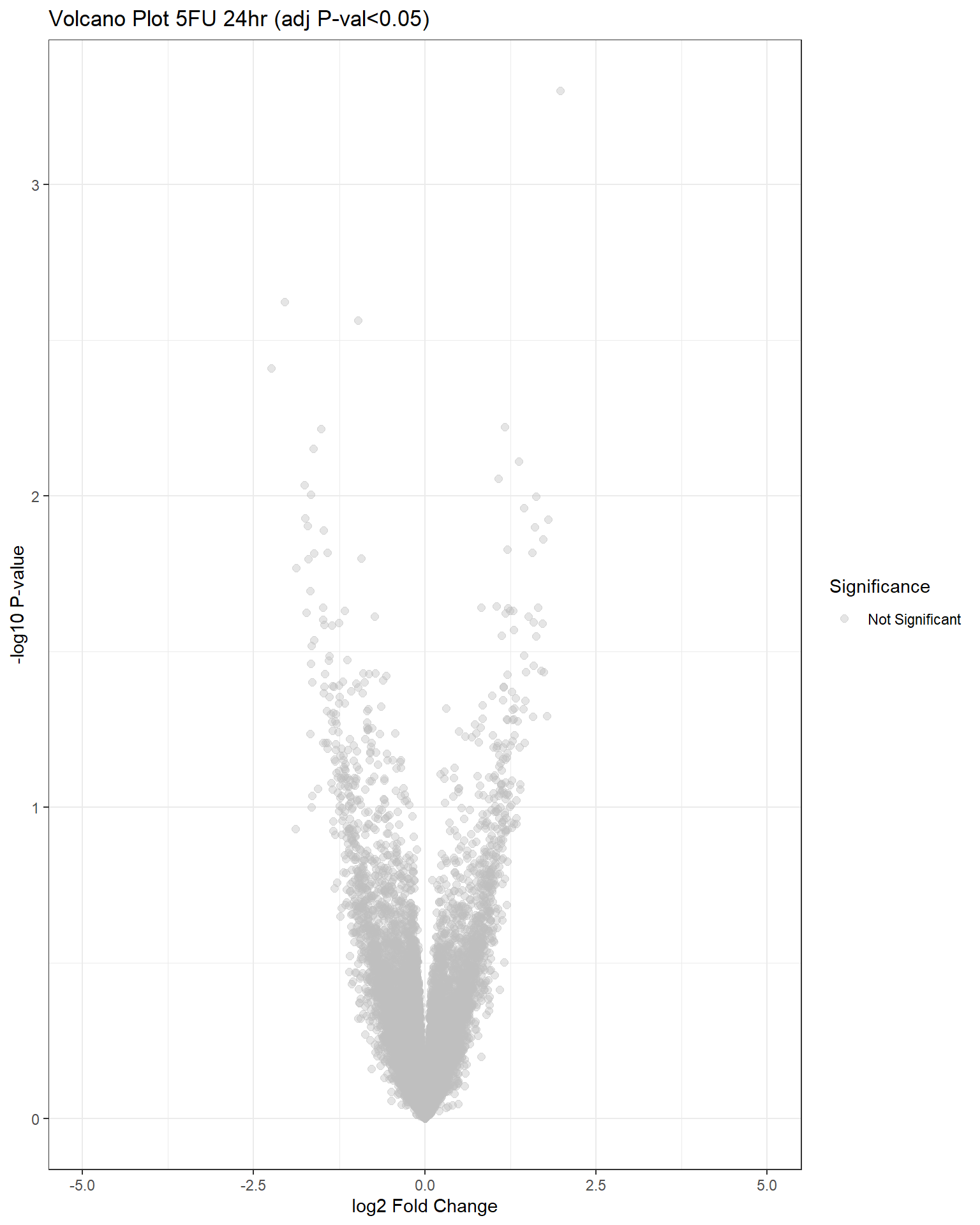
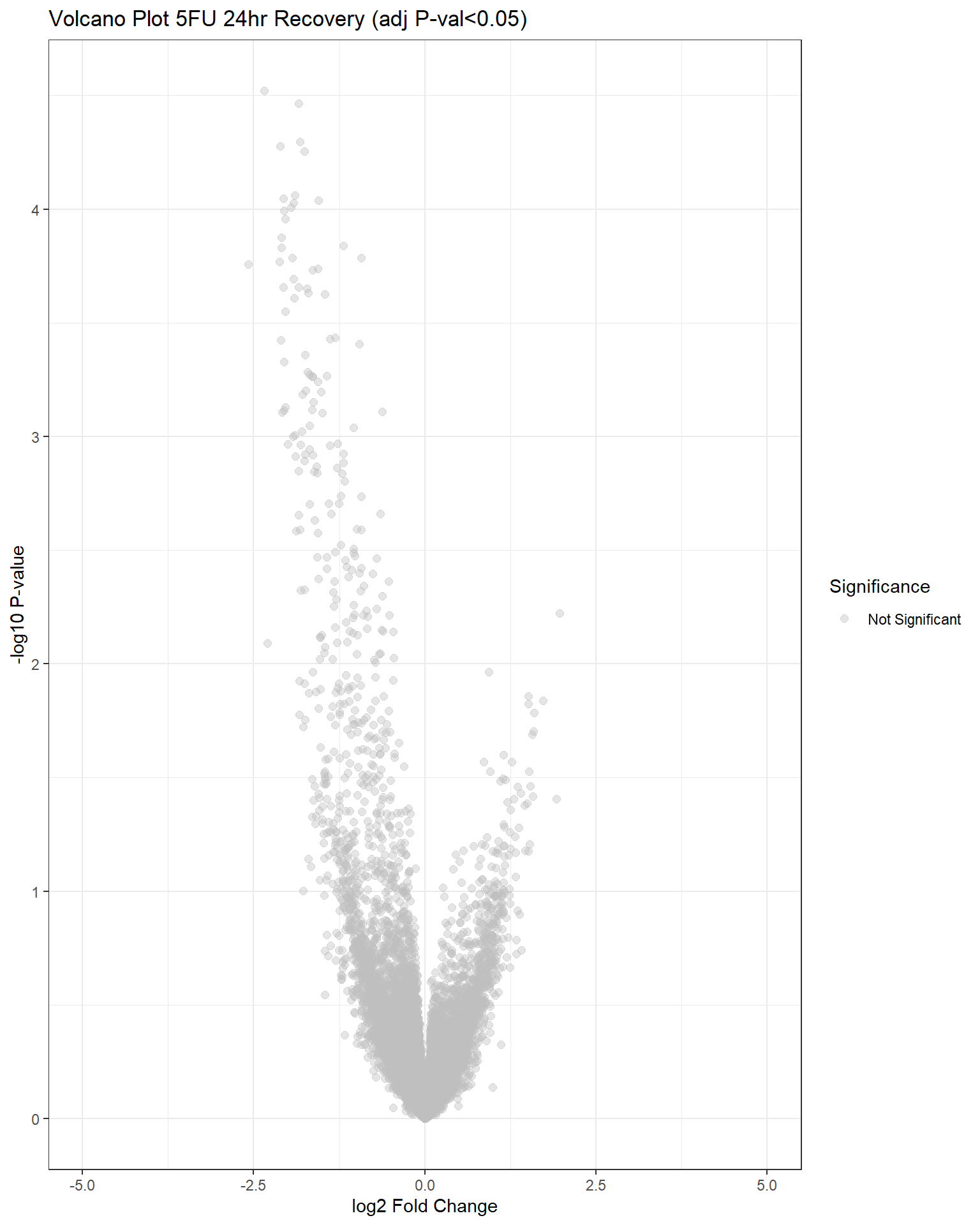
## have no DE genes detected for 5FU, only DOX
####plot your voom####
voom_plot1 <- voom(dge1_calc, mm_r1, plot = TRUE)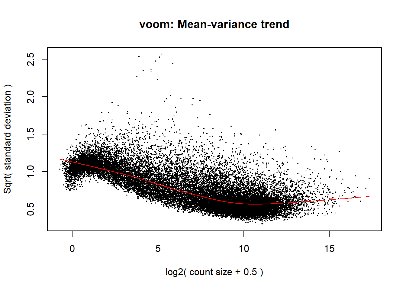
top.table_V.D24 <- topTable(fit = efit4, coef = "V.D24", number = nrow(dge_calc), adjust.method = "BH", p.value = 1, sort.by = "none")
head(top.table_V.D24)

top.table_V.F24 <- topTable(fit = efit4, coef = "V.F24", number = nrow(dge_calc), adjust.method = "BH", p.value = 1, sort.by = "none")
head(top.table_V.F24)

top.table_V.D24r <- topTable(fit = efit4, coef = "V.D24r", number = nrow(dge_calc), adjust.method = "BH", p.value = 1, sort.by = "none")
head(top.table_V.D24r)

top.table_V.F24r <- topTable(fit = efit4, coef = "V.F24r", number = nrow(dge_calc), adjust.method = "BH", p.value = 1, sort.by = "none")
head(top.table_V.F24r)

top.table_V.D144r <- topTable(fit = efit4, coef = "V.D144r", number = nrow(dge_calc), adjust.method = "BH", p.value = 1, sort.by = "none")
head(top.table_V.D144r)

top.table_V.F144r <- topTable(fit = efit4, coef = "V.F144r", number = nrow(dge_calc), adjust.method = "BH", p.value = 1, sort.by = "none")
head(top.table_V.F144r)
Volcano Plots
generate_volcano_plot <- function(toptable, title) {
# Add Significance Labels
toptable$Significance <- "Not Significant"
toptable$Significance[toptable$logFC > 0 & toptable$adj.P.Val < 0.05] <- "Upregulated"
toptable$Significance[toptable$logFC < 0 & toptable$adj.P.Val < 0.05] <- "Downregulated"
# Generate Volcano Plot
ggplot(toptable, aes(x = logFC, y = -log10(P.Value), color = Significance)) +
geom_point(alpha = 0.4, size = 2) +
scale_color_manual(values = c("Downregulated" = "red", "Upregulated" = "blue", "Not Significant" = "gray")) +
xlim(-5, 5) +
labs(title = title, x = "log2 Fold Change", y = "-log10 P-value") +
theme(legend.position = "none",
plot.title = element_text(size = rel(1.5), hjust = 0.5),
axis.title = element_text(size = rel(1.25))) +
theme_bw()
}
#now that I've made a function, I can make volcano plots for each of my comparisons (6 total)
volcano_plots <- list(
"V.D24" = generate_volcano_plot(top.table_V.D24, "Volcano Plot DOX 24hr (adj P-val<0.05)"),
"V.F24" = generate_volcano_plot(top.table_V.F24, "Volcano Plot 5FU 24hr (adj P-val<0.05)"),
"V.D24r" = generate_volcano_plot(top.table_V.D24r, "Volcano Plot DOX 24hr Recovery (adj P-val<0.05)"),
"V.F24r" = generate_volcano_plot(top.table_V.F24r, "Volcano Plot 5FU 24hr Recovery (adj P-val<0.05)"),
"V.D144r" = generate_volcano_plot(top.table_V.D144r, "Volcano Plot DOX 6d Recovery (adj P-val<0.05)"),
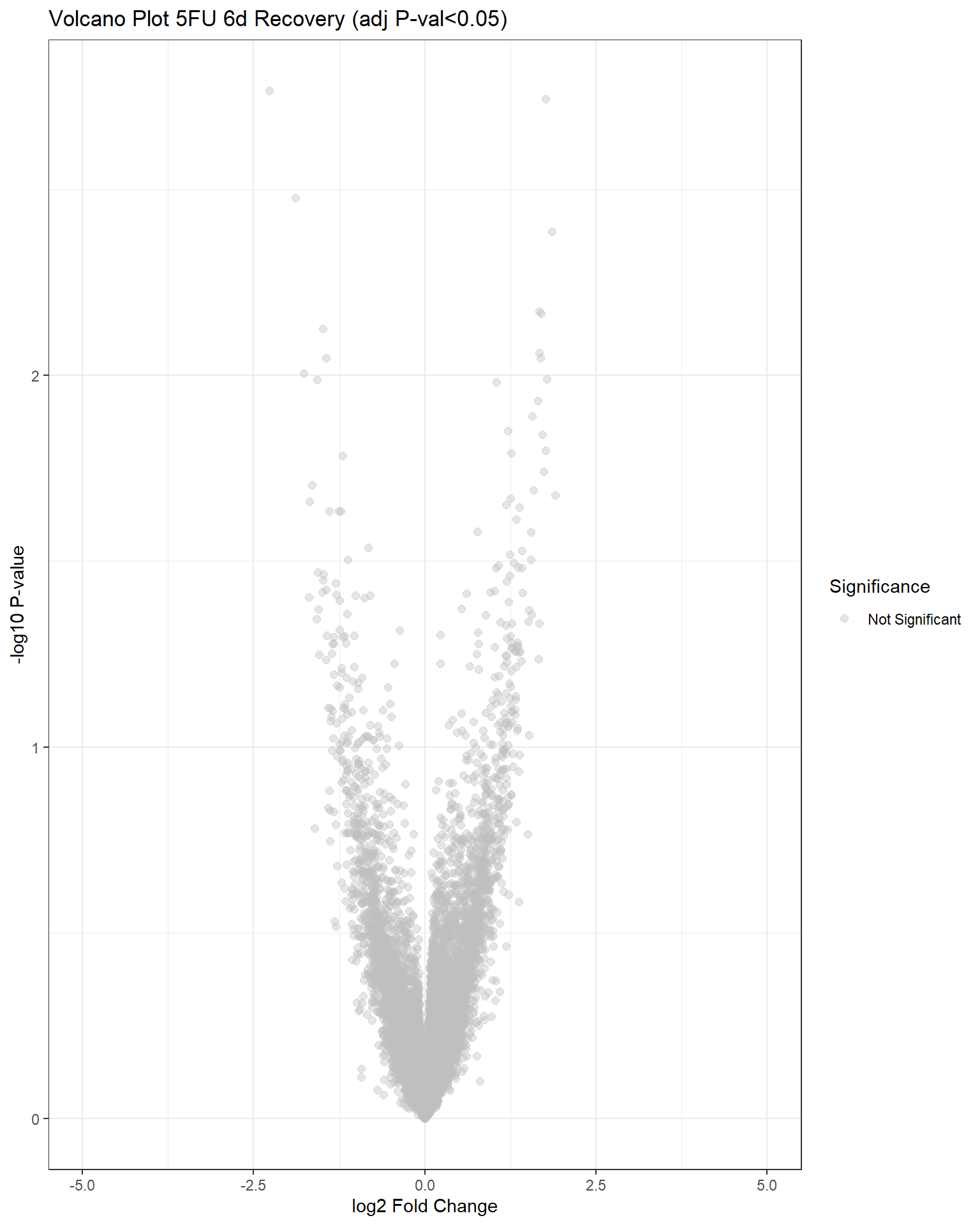
"V.F144r" = generate_volcano_plot(top.table_V.F144r, "Volcano Plot 5FU 6d Recovery (adj P-val<0.05)")
)
# Display each volcano plot
for (plot_name in names(volcano_plots)) {
print(volcano_plots[[plot_name]])
}
Warning: Removed 344 rows containing missing values or values outside the scale range
(`geom_point()`).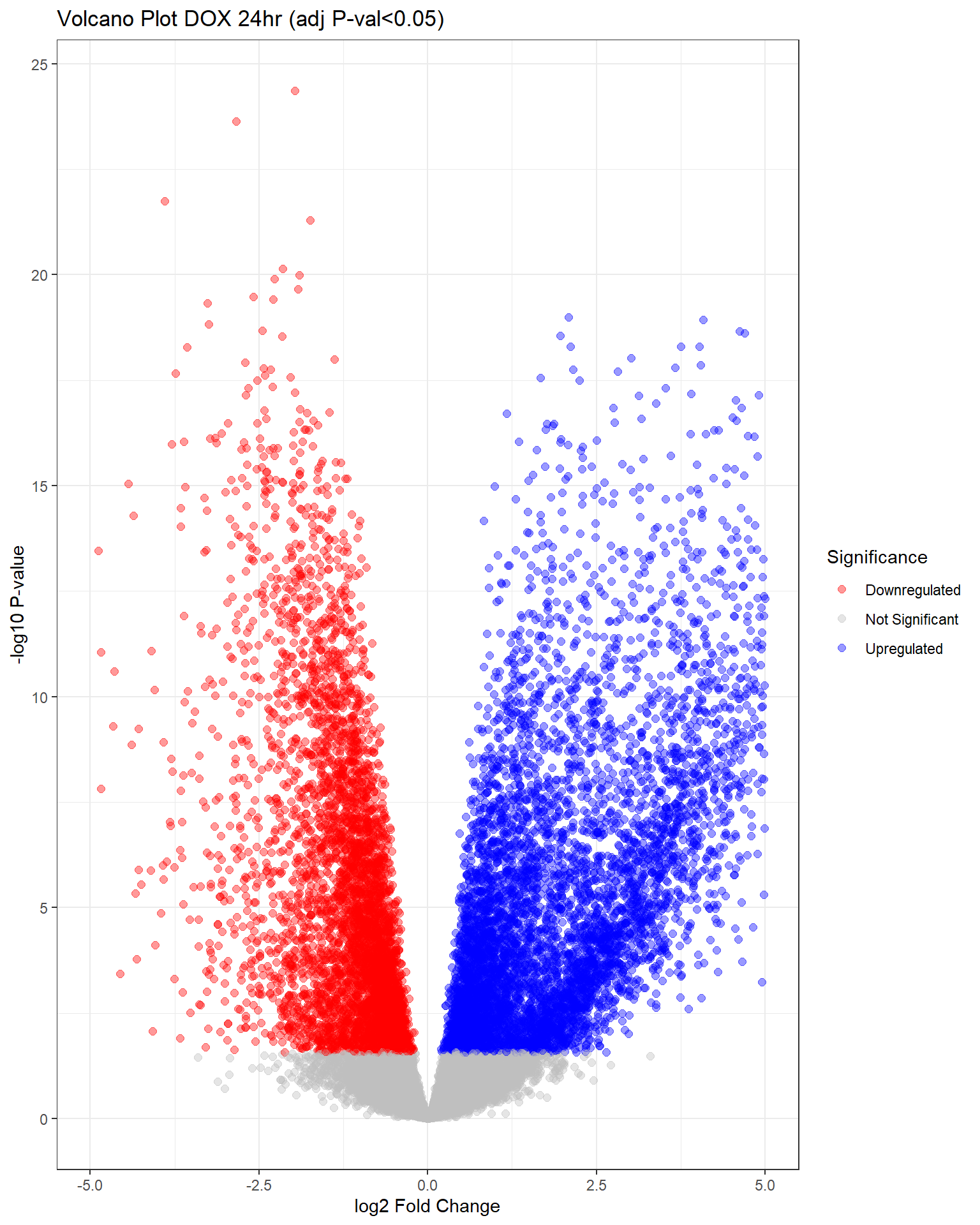
Warning: Removed 66 rows containing missing values or values outside the scale range
(`geom_point()`).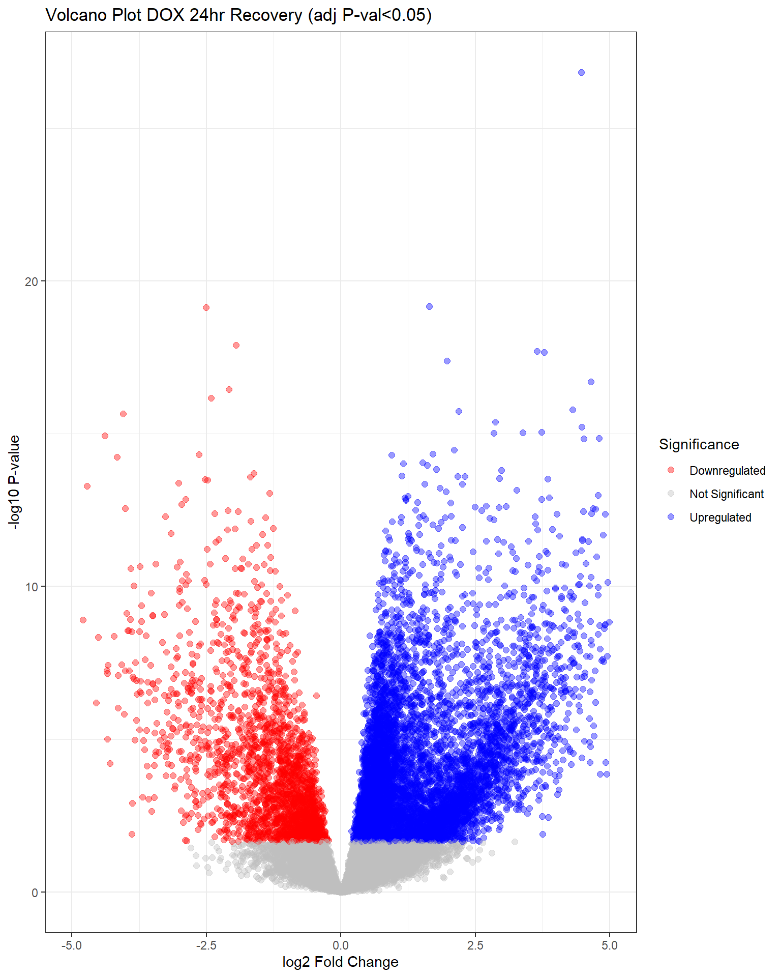
Warning: Removed 23 rows containing missing values or values outside the scale range
(`geom_point()`).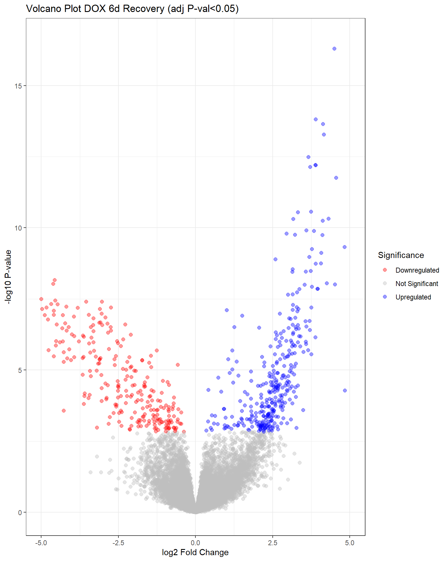
Now that I’ve gone through and figured out the basics of DE - let’s remove unwanted variation using ruv This uses my replicates to figure out covariates in the data and remove variation occurring due to batch effects or other effects We’re seeing a batch effect occurring here in PCA and cor. heatmaps
# #counts need to be integer values and in a numeric matrix for ruv
# counts_DE_matrix <- as.matrix(counts_DE_filter1)
# dim(counts_DE_matrix)
# #[1] 20443    54 - new inbuilt
# #this does NOT contain the replicate samples, save for later
#
# ##this file contains the replicates that I can pull from
# fC_Matrix_cpm_filter_ruv <- as.matrix (fC_Matrix_Full_cpm_filter)
#
# #create a matrix specifying the replicates
# reps <- as.data.frame(fC_Matrix_Full_cpm_filter) %>%
#   dplyr::select(contains("Ind6"))
# dim(reps)
# #[1] 14225    18
# reps_mat <- as.matrix(reps)
#
# #using the documentation do this:
# #controls: gene-by-sample numeric matrix containing counts
# controls <- rownames(fC_Matrix_Full_cpm_filter)
#
# #I have replicates for Individual 6, which I can compare using this method
# #They are matched as following:
# ##col46:55, 47:56, 48:57, 49:58, 50:59, 51:60, 52:61, 53:62, 54:63
# ###this is the scIdx argument for reps, the cIdx argument is for genes
# #differences <- matrix(data = c(1, 10, 2, 11, 3, 12, 4, 13, 5, 14, 6, 15, 7, 16, 8, 17, 9, 18), byrow = TRUE, nrow = 9)
# differences_full <- matrix(data = c(46, 55, 47, 56, 48 , 57, 49, 58, 50 , 59, 51, 60, 52, 61, 53, 62, 54, 63), byrow = TRUE, nrow = 9)
#
#
# signature(x = "matrix", cIdx = "ANY", k = "numeric", scIdx = "matrix")
#
#
# seqRUVs <- RUVs(rep, controls, k=3, differences_full, isLog = TRUE)
#
# pData(counts_DE)
# head(seqRUVs)
#
#
# ###now try putting this in your matrix?
# design <- model.matrix(~0 + group_1, seqRUVs)
#
#
#
#
# ####try it exactly like the documentation and filter afterwards?####
# genes <- rownames(fC_Matrix_Full)[grep("^"), rownames(fC_Matrix_Full)]
# spikes <- rownames()
#
# ####leaving off here EMP 25/02/26####
sessionInfo()R version 4.4.2 (2024-10-31 ucrt)
Platform: x86_64-w64-mingw32/x64
Running under: Windows 11 x64 (build 22000)
Matrix products: default
locale:
[1] LC_COLLATE=English_United States.utf8
[2] LC_CTYPE=English_United States.utf8
[3] LC_MONETARY=English_United States.utf8
[4] LC_NUMERIC=C
[5] LC_TIME=English_United States.utf8
time zone: America/Chicago
tzcode source: internal
attached base packages:
[1] stats4 stats graphics grDevices utils datasets methods
[8] base
other attached packages:
[1] RUVSeq_1.40.0 EDASeq_2.40.0
[3] ShortRead_1.64.0 GenomicAlignments_1.42.0
[5] SummarizedExperiment_1.36.0 MatrixGenerics_1.18.1
[7] matrixStats_1.4.1 Rsamtools_2.22.0
[9] GenomicRanges_1.58.0 Biostrings_2.74.0
[11] GenomeInfoDb_1.42.3 XVector_0.46.0
[13] IRanges_2.40.0 S4Vectors_0.44.0
[15] BiocParallel_1.40.0 biomaRt_2.62.1
[17] RColorBrewer_1.1-3 Cormotif_1.52.0
[19] affy_1.84.0 Biobase_2.66.0
[21] BiocGenerics_0.52.0 PCAtools_2.18.0
[23] ggrepel_0.9.6 ggfortify_0.4.17
[25] pheatmap_1.0.12 edgeR_4.4.0
[27] limma_3.62.1 readxl_1.4.3
[29] edgebundleR_0.1.4 lubridate_1.9.3
[31] forcats_1.0.0 stringr_1.5.1
[33] dplyr_1.1.4 purrr_1.0.2
[35] readr_2.1.5 tidyr_1.3.1
[37] tidyverse_2.0.0 tibble_3.2.1
[39] hrbrthemes_0.8.7 reshape2_1.4.4
[41] ggplot2_3.5.1 workflowr_1.7.1
loaded via a namespace (and not attached):
[1] later_1.4.1 BiocIO_1.16.0
[3] bitops_1.0-9 filelock_1.0.3
[5] R.oo_1.27.0 cellranger_1.1.0
[7] preprocessCore_1.68.0 XML_3.99-0.18
[9] lifecycle_1.0.4 httr2_1.1.0
[11] pwalign_1.2.0 rprojroot_2.0.4
[13] vroom_1.6.5 MASS_7.3-61
[15] processx_3.8.5 lattice_0.22-6
[17] magrittr_2.0.3 sass_0.4.9
[19] rmarkdown_2.29 jquerylib_0.1.4
[21] yaml_2.3.10 httpuv_1.6.15
[23] cowplot_1.1.3 DBI_1.2.3
[25] abind_1.4-8 zlibbioc_1.52.0
[27] R.utils_2.12.3 RCurl_1.98-1.16
[29] rappdirs_0.3.3 git2r_0.35.0
[31] gdtools_0.4.1 GenomeInfoDbData_1.2.13
[33] irlba_2.3.5.1 dqrng_0.4.1
[35] DelayedMatrixStats_1.28.1 codetools_0.2-20
[37] DelayedArray_0.32.0 xml2_1.3.6
[39] tidyselect_1.2.1 farver_2.1.2
[41] UCSC.utils_1.2.0 ScaledMatrix_1.14.0
[43] BiocFileCache_2.14.0 jsonlite_1.8.9
[45] systemfonts_1.1.0 tools_4.4.2
[47] progress_1.2.3 Rcpp_1.0.13-1
[49] glue_1.8.0 gridExtra_2.3
[51] Rttf2pt1_1.3.12 SparseArray_1.6.0
[53] xfun_0.49 withr_3.0.2
[55] BiocManager_1.30.25 fastmap_1.2.0
[57] latticeExtra_0.6-30 callr_3.7.6
[59] digest_0.6.37 rsvd_1.0.5
[61] timechange_0.3.0 R6_2.6.1
[63] mime_0.12 colorspace_2.1-1
[65] jpeg_0.1-10 RSQLite_2.3.8
[67] R.methodsS3_1.8.2 generics_0.1.3
[69] fontLiberation_0.1.0 rtracklayer_1.66.0
[71] prettyunits_1.2.0 httr_1.4.7
[73] htmlwidgets_1.6.4 S4Arrays_1.6.0
[75] whisker_0.4.1 pkgconfig_2.0.3
[77] gtable_0.3.6 blob_1.2.4
[79] hwriter_1.3.2.1 htmltools_0.5.8.1
[81] fontBitstreamVera_0.1.1 scales_1.3.0
[83] png_0.1-8 knitr_1.49
[85] rstudioapi_0.17.1 tzdb_0.4.0
[87] rjson_0.2.23 curl_6.0.1
[89] cachem_1.1.0 parallel_4.4.2
[91] extrafont_0.19 AnnotationDbi_1.68.0
[93] restfulr_0.0.15 pillar_1.10.1
[95] grid_4.4.2 vctrs_0.6.5
[97] promises_1.3.2 BiocSingular_1.22.0
[99] dbplyr_2.5.0 beachmat_2.22.0
[101] xtable_1.8-4 extrafontdb_1.0
[103] evaluate_1.0.3 GenomicFeatures_1.58.0
[105] cli_3.6.3 locfit_1.5-9.10
[107] compiler_4.4.2 rlang_1.1.4
[109] crayon_1.5.3 labeling_0.4.3
[111] aroma.light_3.36.0 interp_1.1-6
[113] ps_1.8.1 getPass_0.2-4
[115] plyr_1.8.9 fs_1.6.5
[117] stringi_1.8.4 deldir_2.0-4
[119] munsell_0.5.1 fontquiver_0.2.1
[121] Matrix_1.7-1 hms_1.1.3
[123] sparseMatrixStats_1.18.0 bit64_4.5.2
[125] KEGGREST_1.46.0 statmod_1.5.0
[127] shiny_1.10.0 igraph_2.1.1
[129] memoise_2.0.1 affyio_1.76.0
[131] bslib_0.9.0 bit_4.5.0