GWAS tutorial
Fabio Morgante
August 28, 2024
Last updated: 2024-08-28
Checks: 7 0
Knit directory: gwas_tutorial/
This reproducible R Markdown analysis was created with workflowr (version 1.7.1). The Checks tab describes the reproducibility checks that were applied when the results were created. The Past versions tab lists the development history.
Great! Since the R Markdown file has been committed to the Git repository, you know the exact version of the code that produced these results.
Great job! The global environment was empty. Objects defined in the global environment can affect the analysis in your R Markdown file in unknown ways. For reproduciblity it’s best to always run the code in an empty environment.
The command set.seed(20240828) was run prior to running
the code in the R Markdown file. Setting a seed ensures that any results
that rely on randomness, e.g. subsampling or permutations, are
reproducible.
Great job! Recording the operating system, R version, and package versions is critical for reproducibility.
Nice! There were no cached chunks for this analysis, so you can be confident that you successfully produced the results during this run.
Great job! Using relative paths to the files within your workflowr project makes it easier to run your code on other machines.
Great! You are using Git for version control. Tracking code development and connecting the code version to the results is critical for reproducibility.
The results in this page were generated with repository version f985e97. See the Past versions tab to see a history of the changes made to the R Markdown and HTML files.
Note that you need to be careful to ensure that all relevant files for
the analysis have been committed to Git prior to generating the results
(you can use wflow_publish or
wflow_git_commit). workflowr only checks the R Markdown
file, but you know if there are other scripts or data files that it
depends on. Below is the status of the Git repository when the results
were generated:
Ignored files:
    Ignored:    .DS_Store
    Ignored:    .Rhistory

Untracked files:
    Untracked:  data/RiceDiversity.44K.germplasm.csv
    Untracked:  data/RiceDiversity_44K_Phenotypes_34traits_PLINK.txt
    Untracked:  data/sativas413.fam
    Untracked:  data/sativas413.map
    Untracked:  data/sativas413.ped

Unstaged changes:
    Modified:   analysis/_site.yml
Note that any generated files, e.g. HTML, png, CSS, etc., are not included in this status report because it is ok for generated content to have uncommitted changes.
These are the previous versions of the repository in which changes were
made to the R Markdown (analysis/gwas_rice.Rmd) and HTML
(docs/gwas_rice.html) files. If you’ve configured a remote
Git repository (see ?wflow_git_remote), click on the
hyperlinks in the table below to view the files as they were in that
past version.
| File | Version | Author | Date | Message |
|---|---|---|---|---|
| Rmd | f985e97 | fmorgante | 2024-08-28 | Add rice tutorial |
This tutorial is adapted from https://whussain2.github.io/Materials/Teaching/GWAS_R_2.html.
##Description of the data
For this tutorial, we will use rice data that can be dowloaded here. These data include genotypes at ~44K SNPs and 36 phenotypes for 413 accessions of Oryza sativa. More details about these data can be found in this paper.
##Load libraies needed
First, we will load the necessary R packages, BGLR, SNPRelate, dplyr, rrBLUP, and qqman.
library(BGLR)
library(SNPRelate)
Loading required package: gdsfmtSNPRelatelibrary(dplyr)
Attaching package: 'dplyr'The following objects are masked from 'package:stats':
filter, lagThe following objects are masked from 'package:base':
intersect, setdiff, setequal, unionlibrary(rrBLUP)
library(qqman)For example usage please run: vignette('qqman')Citation appreciated but not required:Turner, (2018). qqman: an R package for visualizing GWAS results using Q-Q and manhattan plots. Journal of Open Source Software, 3(25), 731, https://doi.org/10.21105/joss.00731.##Prepare genotype and phenotype data
The genotype data are included in three files with extension .fam (which includes information about the samples), .map (which contains information about the SNPs, such as chromosome and position), .ped (which contains the genotype calls, where 0 and 3 mean homozygous for either allele, 1 means heterozygous, and 2 means missing). For our purpose, we will recode missing geneotype as NA and heterozygous genotypes as 1.
###Load genotype file
geno <- read_ped("data/sativas413.ped")
FAM <- read.table("data/sativas413.fam", header=FALSE, sep=" ")
MAP <- read.table("data/sativas413.map", header=FALSE, sep="\t")

p <- geno$p
n <- geno$n

###Access genotype matrix
geno_vec <- geno$x

###Recode genotypes
geno_vec[geno_vec == 2] <- NA  # Converting missing data to NA
geno_vec[geno_vec == 3] <- 2  # Converting 3 to 2

###Convert the genotype data into matrix, transpose and check dimensions
geno_mat <- matrix(geno_vec, nrow = p, ncol = n, byrow = TRUE)
geno_mat <- t(geno_mat)
dim(geno_mat)
[1] 413 36901colnames(geno_mat) <- MAP$V2
rownames(geno_mat) <- FAM$V2
dim(geno_mat)[1] 413 36901geno_mat[1:5, 1:5] id1000001 id1000003 id1000005 id1000007 id1000008
1 0 0 0 0 0
3 2 2 0 2 2
4 2 2 0 2 2
5 2 2 2 0 2
6 2 2 0 2 2From the phenotype data, we selected Flowering.time.at.Aberdeen as our trait of interest. Note that NSFTVID is the ID of the accession and missing value are coded as NA. Accessions with missing phenotype are removed.
###Load phenotype data
rice_pheno <- read.table("data/RiceDiversity_44K_Phenotypes_34traits_PLINK.txt",
                         header = TRUE, stringsAsFactors = FALSE, sep = "\t")

###Extract phenotype and remove missing values
y <- rice_pheno$Flowering.time.at.Aberdeen
index <- !is.na(y)
y <- data.frame(NSFTV.ID = rice_pheno$NSFTVID[index], y = y[index])

dim(y)
[1] 359 2head(y) NSFTV.ID y
1 1 81
2 3 83
3 4 93
4 5 108
5 6 101
6 7 158Let’s now do some QC on the genotype data. This includes removing accessions with missing phenotype, computing minor allele frequency (MAF) for each SNP, and removing SNPs with MAF smaller than 0.05.
###Remove accessions with missing pheno
geno_mat <- geno_mat[index, ]

###Filter out variants with small MAF
af <- colMeans(geno_mat, na.rm = TRUE)/2
maf <- pmin(af, 1-af)
to_remove <- which(maf < 0.05)
geno_mat <- geno_mat[, -to_remove]
MAP <- MAP[-to_remove, ]

dim(geno_mat)
[1] 359 33572##Investigation of population structure
These accessions come from different populations. The presence of population structure can induce false positives, so we need to investigate this. To do so, we will build a genomic relationship matrix (GRM) that measures the similarity between accessions based genotypes. The higher the coefficient of genomic relationship, the more similar two accessions are.
###Create gds format file and save it as 44k.gds
snpgdsCreateGeno("data/44k.gds", genmat = geno_mat, sample.id = rownames(geno_mat), snp.id = colnames(geno_mat),
                 snp.chromosome = MAP$V1, snp.position = MAP$V4, snpfirstdim = FALSE)
# Now open the 44k.gds file
geno_44k <- snpgdsOpen("data/44k.gds")
snpgdsSummary("data/44k.gds")
The file name: /Users/fabiom/Documents/GIT/gwas_tutorial/data/44k.gds
The total number of samples: 359
The total number of SNPs: 33572
SNP genotypes are stored in SNP-major mode (Sample X SNP).###Compute GRM
grm_obj <- snpgdsGRM(geno_44k, method="GCTA")Genetic Relationship Matrix (GRM, GCTA):
Excluding 0 SNP on non-autosomes
Excluding 0 SNP (monomorphic: TRUE, MAF: NaN, missing rate: NaN)
# of samples: 359
# of SNPs: 33,572
using 1 thread
GRM Calculation: the sum of all selected genotypes (0,1,2) = 7149883
CPU capabilities:
Wed Aug 28 10:44:50 2024 (internal increment: 1368)
[..................................................] 0%, ETC: --- [==================================================] 100%, completed, 2s
Wed Aug 28 10:44:52 2024 Done.GRM <- grm_obj$grm
colnames(GRM) <- rownames(GRM) <- grm_obj$sample.id
dim(GRM)[1] 359 359GRM[1:5, 1:5] 1 3 4 5 6
1 1.3019512 -1.0096800 -0.8575139 0.0078842 -0.8105344
3 -1.0096800 3.1219327 0.7288741 -0.2955218 0.6856645
4 -0.8575139 0.7288741 2.8092981 -0.1398424 2.3414236
5 0.0078842 -0.2955218 -0.1398424 1.7246536 -0.1352005
6 -0.8105344 0.6856645 2.3414236 -0.1352005 2.7222408We will perform principal component analysis (PCA) via eigen decomposition of the GRM, to determine whether population structure is actually present.
###Perform eigen decomposition
eig <- eigen(GRM)

eig_vectors <- eig$vectors
colnames(eig_vectors) <- paste0("EV", 1:ncol(eig_vectors))
eig_vectors_df <- data.frame(NSFTV.ID = grm_obj$sample.id, eig_vectors)

###Plot PC1 vs PC2 and label points according to the pop they belong to
plot(eig_vectors_df$EV1, eig_vectors_df$EV2, xlab = "PC1", ylab = "PC2")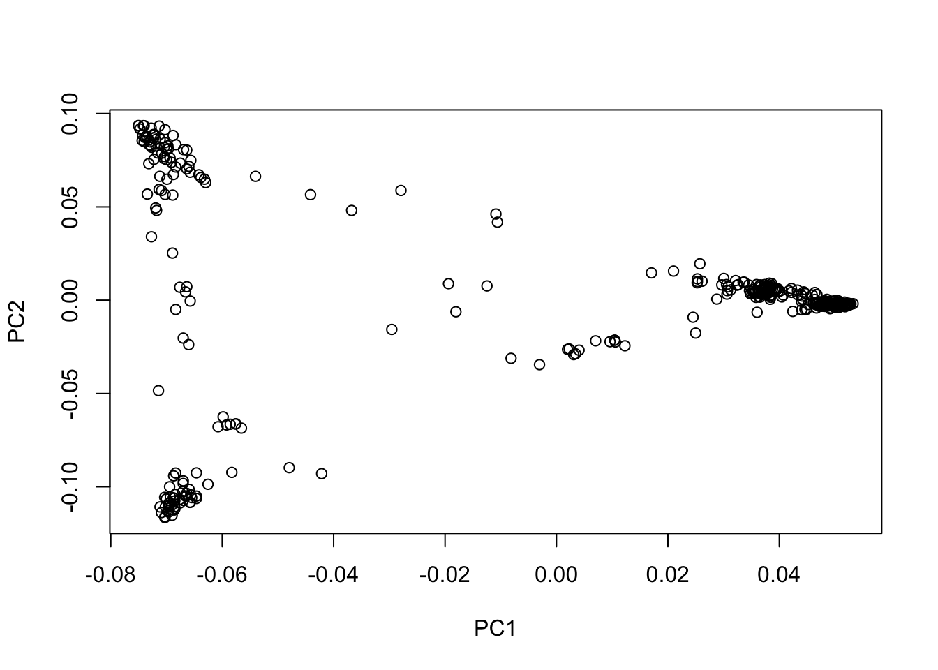
From the plot of PC1 vs PC2, we can see that there is indeed population structure, with groups of accessions being closer to each other than to the rest. This becomes even more clear when we overlay information about the population that each accession comes from.
###Add population info from the web to PC data
pop_info <- read.csv("data/RiceDiversity.44K.germplasm.csv",
                     header = TRUE, skip = 1, stringsAsFactors = FALSE)
pop_info <- pop_info[, c("NSFTV.ID", "Sub.population")]
pop_info$NSFTV.ID <- as.character(pop_info$NSFTV.ID)

eig_vectors_info <- left_join(eig_vectors_df, pop_info, by="NSFTV.ID")

###Plot PC1 vs PC2 and label points according to the pop they belong to
plot(eig_vectors_info$EV1, eig_vectors_info$EV2, xlab = "PC1", ylab = "PC2", col = c(1:6)[factor(eig_vectors_info$Sub.population)])
legend(x = "topright", legend = levels(factor(eig_vectors_info$Sub.population)), col = c(1:6),
       pch = 1, cex = 0.6)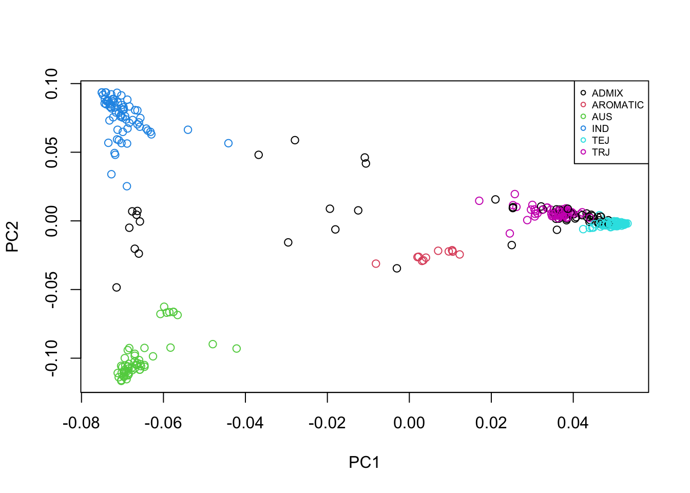
##Genome-Wide Association Study
We will now perform a GWAS for our trait of interest using a linear mixed model that models the covariance between accessions (our random effect) using the GRM. That way, we correct for population structure.
###Make the GRM positive semi-definite
eig_values <- eig$values
eig_values[eig_values<0] <- 0
GRM_SPD <- eig_vectors %*% diag(eig_values) %*% t(eig_vectors)

###Prepare genotype data in the format expected by rrBLUP
geno_final <- data.frame(marker = MAP[, 2], chrom = MAP[, 1], pos = MAP[, 4],
                         t(geno_mat - 1), check.names = FALSE)  # W = \in{-1, 0, 1}

###Perform GWAS via linear mixed model
results <- GWAS(pheno=y, geno=geno_final, K=GRM_SPD, min.MAF=0, P3D = TRUE, plot = FALSE)
[1] "GWAS for trait: y"
[1] "Variance components estimated. Testing markers."results$p_value <- 10^(-results$y)The results are displayed as a Q-Q plot, where the observed p-values are plotted against the expected p-values under the null hypothesis of no association between the SNP and the phenotype.
###Make qqplot
qq(results$p_value)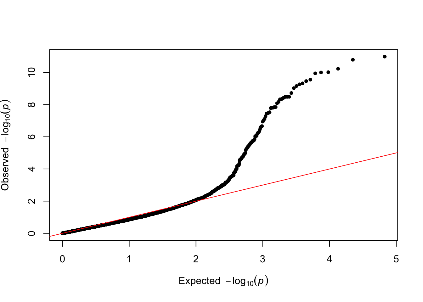
This plot looks pretty good – large observed p-values are well aligned to their expectation under the null, while smaller p-valuesshow a deviation from their expectation under the null, hinting at discovering true signals. We then display the final results as a manhattan plot, where the significance line reflects a Bonferroni correction.
###Make qqplot
manhattan(results, chr="chrom", bp="pos", p="p_value", snp = "marker",
          genomewideline = -log10(0.05/nrow(geno_final)), suggestiveline=FALSE)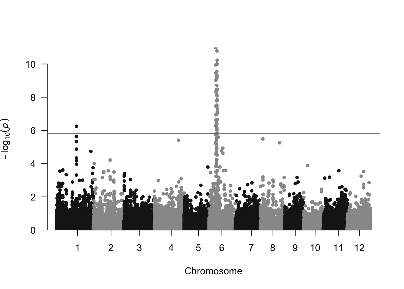
It looks like there is a strong association signal on chromosome 6, and a weaker one on chromosome 1.
As an exercise, what if we had done GWAS with a regular linear model disregarding population structure?
###Perform GWAS via simple linear regression
results$p_value_lm <- as.numeric(NA)

# This is slow code that is only useful for the teaching purpose
for(i in 1:nrow(geno_final)){
  fit <- lm(y$y ~ as.numeric(geno_final[i, 4:ncol(geno_final)]))
  results[i, "p_value_lm"] <- summary(fit)$coefficients[2,4]
}

qq(results$p_value_lm)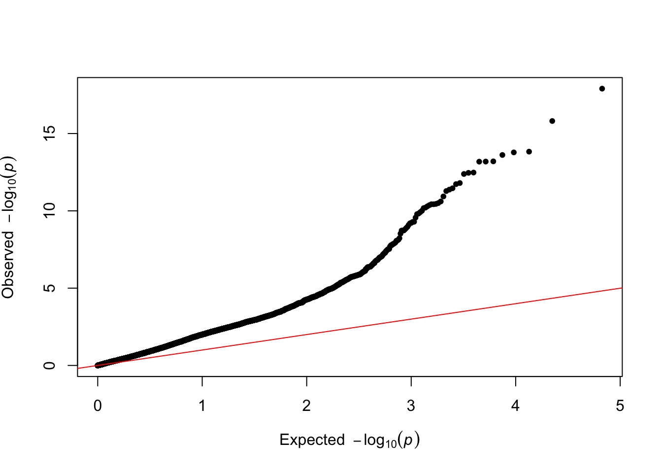
The Q-Q plot looks pretty bad now, with clear signs of uncorrected confounding.
sessionInfo()R version 4.2.1 (2022-06-23)
Platform: aarch64-apple-darwin20 (64-bit)
Running under: macOS Monterey 12.7.6
Matrix products: default
LAPACK: /Library/Frameworks/R.framework/Versions/4.2-arm64/Resources/lib/libRlapack.dylib
locale:
[1] en_US.UTF-8/en_US.UTF-8/en_US.UTF-8/C/en_US.UTF-8/en_US.UTF-8
attached base packages:
[1] stats graphics grDevices utils datasets methods base
other attached packages:
[1] qqman_0.1.9 rrBLUP_4.6.3 dplyr_1.1.4 SNPRelate_1.32.2
[5] gdsfmt_1.34.1 BGLR_1.1.2 workflowr_1.7.1
loaded via a namespace (and not attached):
[1] Rcpp_1.0.12 highr_0.11 compiler_4.2.1 pillar_1.9.0
[5] bslib_0.8.0 later_1.3.2 git2r_0.33.0 jquerylib_0.1.4
[9] tools_4.2.1 getPass_0.2-4 digest_0.6.35 jsonlite_1.8.8
[13] evaluate_0.24.0 lifecycle_1.0.4 tibble_3.2.1 pkgconfig_2.0.3
[17] rlang_1.1.3 cli_3.6.2 rstudioapi_0.16.0 parallel_4.2.1
[21] yaml_2.3.8 xfun_0.44 fastmap_1.2.0 httr_1.4.7
[25] stringr_1.5.1 knitr_1.48 generics_0.1.3 fs_1.6.4
[29] vctrs_0.6.5 sass_0.4.9 tidyselect_1.2.1 rprojroot_2.0.4
[33] calibrate_1.7.7 glue_1.7.0 R6_2.5.1 processx_3.8.4
[37] fansi_1.0.6 rmarkdown_2.28 callr_3.7.6 magrittr_2.0.3
[41] whisker_0.4.1 MASS_7.3-57 ps_1.7.6 promises_1.3.0
[45] htmltools_0.5.8.1 httpuv_1.6.15 utf8_1.2.4 stringi_1.8.4
[49] truncnorm_1.0-9 cachem_1.1.0