Dense case (larger sample size)
Fabio Morgante
June 03, 2020
Last updated: 2020-06-03
Checks: 7 0
Knit directory: mr_mash_test/
This reproducible R Markdown analysis was created with workflowr (version 1.6.1). The Checks tab describes the reproducibility checks that were applied when the results were created. The Past versions tab lists the development history.
Great! Since the R Markdown file has been committed to the Git repository, you know the exact version of the code that produced these results.
Great job! The global environment was empty. Objects defined in the global environment can affect the analysis in your R Markdown file in unknown ways. For reproduciblity it’s best to always run the code in an empty environment.
The command set.seed(20200328) was run prior to running the code in the R Markdown file. Setting a seed ensures that any results that rely on randomness, e.g. subsampling or permutations, are reproducible.
Great job! Recording the operating system, R version, and package versions is critical for reproducibility.
Nice! There were no cached chunks for this analysis, so you can be confident that you successfully produced the results during this run.
Great job! Using relative paths to the files within your workflowr project makes it easier to run your code on other machines.
Great! You are using Git for version control. Tracking code development and connecting the code version to the results is critical for reproducibility.
The results in this page were generated with repository version 33806cd. See the Past versions tab to see a history of the changes made to the R Markdown and HTML files.
Note that you need to be careful to ensure that all relevant files for the analysis have been committed to Git prior to generating the results (you can use wflow_publish or wflow_git_commit). workflowr only checks the R Markdown file, but you know if there are other scripts or data files that it depends on. Below is the status of the Git repository when the results were generated:
Ignored files:
    Ignored:    .sos/
    Ignored:    code/fit_mr_mash.66662433.err
    Ignored:    code/fit_mr_mash.66662433.out
    Ignored:    dsc/.sos/
    Ignored:    dsc/outfiles/
    Ignored:    output/dsc.html
    Ignored:    output/dsc/
    Ignored:    output/dsc_05_18_20.html
    Ignored:    output/dsc_05_18_20/
    Ignored:    output/dsc_05_29_20.html
    Ignored:    output/dsc_05_29_20/
    Ignored:    output/dsc_OLD.html
    Ignored:    output/dsc_OLD/
    Ignored:    output/dsc_test.html
    Ignored:    output/dsc_test/

Untracked files:
    Untracked:  code/plot_test.R

Unstaged changes:
    Modified:   dsc/midway2.yml
Note that any generated files, e.g. HTML, png, CSS, etc., are not included in this status report because it is ok for generated content to have uncommitted changes.
These are the previous versions of the repository in which changes were made to the R Markdown (analysis/dense_scenario_issue_larger_sample.Rmd) and HTML (docs/dense_scenario_issue_larger_sample.html) files. If you’ve configured a remote Git repository (see ?wflow_git_remote), click on the hyperlinks in the table below to view the files as they were in that past version.
| File | Version | Author | Date | Message |
|---|---|---|---|---|
| Rmd | 33806cd | fmorgante | 2020-06-03 | Add dense scenario with larger sample size |
library(mr.mash.alpha)
library(glmnet)
Loading required package: MatrixLoading required package: foreachLoaded glmnet 2.0-16###Set options
options(stringsAsFactors = FALSE)
###Function to compute accuracy
compute_accuracy <- function(Y, Yhat) {
bias <- rep(as.numeric(NA), ncol(Y))
r2 <- rep(as.numeric(NA), ncol(Y))
mse <- rep(as.numeric(NA), ncol(Y))
for(i in 1:ncol(Y)){
fit <- lm(Y[, i] ~ Yhat[, i])
bias[i] <- coef(fit)[2]
r2[i] <- summary(fit)$r.squared
mse[i] <- mean((Y[, i] - Yhat[, i])^2)
}
return(list(bias=bias, r2=r2, mse=mse))
}Dense scenario
Here we investigate why mr.mash does not perform as well in denser scenarios. Let’s simulate data with n=1000, p=1,000, p_causal=500, r=5, r_causal=5, PVE=0.5, shared effects, independent predictors, and independent residuals. The models will be fitted to the training data (50% of the full data).
###Set seed
set.seed(123)

###Set parameters
n <- 1000
p <- 1000
p_causal <- 500
r <- 5
r_causal <- r
pve <- 0.5
B_cor <- 1
X_cor <- 0
V_cor <- 0

###Simulate V, B, X and Y
out <- mr.mash.alpha:::simulate_mr_mash_data(n, p, p_causal, r, r_causal=r, intercepts = rep(1, r),
                                             pve=pve, B_cor=B_cor, B_scale=0.9, X_cor=X_cor, X_scale=0.8, V_cor=V_cor)

colnames(out$Y) <- paste0("Y", seq(1, r))
rownames(out$Y) <- paste0("N", seq(1, n))
colnames(out$X) <- paste0("X", seq(1, p))
rownames(out$X) <- paste0("N", seq(1, n))

###Split the data in training and test sets
test_set <- sort(sample(x=c(1:n), size=round(n*0.5), replace=FALSE))
Ytrain <- out$Y[-test_set, ]
Xtrain <- out$X[-test_set, ]
Ytest <- out$Y[test_set, ]
Xtest <- out$X[test_set, ]
We build the mixture prior as usual including zero matrix, identity matrix, rank-1 matrices, low, medium and high heterogeneity matrices, shared matrix, each scaled by a grid from 0.1 to 2.1 in steps of 0.2.
grid <- seq(0.1, 2.1, 0.2)
S0 <- mr.mash.alpha:::compute_cov_canonical(ncol(Ytrain), singletons=TRUE, hetgrid=c(0, 0.25, 0.5, 0.75, 1), grid, zeromat=TRUE)
We run glmnet with \(\alpha=1\) to obtain an inital estimate for the regression coefficients to provide to mr.mash, and for comparison.
###Fit group-lasso
cvfit_glmnet <- cv.glmnet(x=Xtrain, y=Ytrain, family="mgaussian", alpha=1)
coeff_glmnet <- coef(cvfit_glmnet, s="lambda.min")
Bhat_glmnet <- matrix(as.numeric(NA), nrow=p, ncol=r)
ahat_glmnet <- vector("numeric", r)
for(i in 1:length(coeff_glmnet)){
  Bhat_glmnet[, i] <- as.vector(coeff_glmnet[[i]])[-1]
  ahat_glmnet[i] <- as.vector(coeff_glmnet[[i]])[1]
}
Yhat_test_glmnet <- drop(predict(cvfit_glmnet, newx=Xtest, s="lambda.min"))
We run mr.mash with EM updates of the mixture weights, updating V, and initializing the regression coefficients with the estimates from glmnet.
###Fit mr.mash
fit_mrmash <- mr.mash(Xtrain, Ytrain, S0, tol=1e-2, convergence_criterion="ELBO", update_w0=TRUE,
                     update_w0_method="EM", compute_ELBO=TRUE, standardize=TRUE, verbose=FALSE, update_V=TRUE,
                     mu1_init = Bhat_glmnet, w0_threshold=1e-8)
Processing the inputs... Done!
Fitting the optimization algorithm... Done!
Processing the outputs... Done!
mr.mash successfully executed in 3.224477 minutes!Yhat_test_mrmash <- predict(fit_mrmash, Xtest)layout(matrix(c(1, 1, 2, 2,
1, 1, 2, 2,
0, 3, 3, 0,
0, 3, 3, 0), 4, 4, byrow = TRUE))
###Plot estimated vs true coeffcients
##mr.mash
plot(out$B, fit_mrmash$mu1, main="mr.mash", xlab="True coefficients", ylab="Estimated coefficients",
cex=2, cex.lab=1.8, cex.main=2, cex.axis=1.8)
##glmnet
plot(out$B, Bhat_glmnet, main="glmnet", xlab="True coefficients", ylab="Estimated coefficients",
cex=2, cex.lab=1.8, cex.main=2, cex.axis=1.8)
###Plot mr.mash vs glmnet estimated coeffcients
colorz <- matrix("black", nrow=p, ncol=r)
zeros <- apply(out$B, 2, function(x) x==0)
for(i in 1:ncol(colorz)){
colorz[zeros[, i], i] <- "red"
}
plot(Bhat_glmnet, fit_mrmash$mu1, main="mr.mash vs glmnet",
xlab="glmnet estimated coefficients", ylab="mr.mash estimated coefficients",
col=colorz, cex=2, cex.lab=1.8, cex.main=2, cex.axis=1.8)
legend("topleft",
legend = c("Non-zero", "Zero"),
col = c("black", "red"),
pch = c(1, 1),
horiz = FALSE,
cex=2) 
print("Prediction performance with glmnet")[1] "Prediction performance with glmnet"compute_accuracy(Ytest, Yhat_test_glmnet)$bias
[1] 0.8512846 1.1180041 1.2579560 1.0588456 0.9750071
$r2
[1] 0.08147787 0.13022180 0.14289736 0.10333887 0.09575056
$mse
[1] 545.7879 564.5279 615.7842 519.2563 549.6524print("Prediction performance with mr.mash")[1] "Prediction performance with mr.mash"compute_accuracy(Ytest, Yhat_test_mrmash)$bias
[1] 0.6516976 0.9183228 0.9410845 0.7707970 0.7797258
$r2
[1] 0.06605585 0.11926910 0.11548491 0.09433716 0.09202714
$mse
[1] 564.6308 571.3867 631.5586 529.2172 556.3545print("True V (full data)")[1] "True V (full data)"out$V [,1] [,2] [,3] [,4] [,5]
[1,] 318.8014 0.0000 0.0000 0.0000 0.0000
[2,] 0.0000 318.8014 0.0000 0.0000 0.0000
[3,] 0.0000 0.0000 318.8014 0.0000 0.0000
[4,] 0.0000 0.0000 0.0000 318.8014 0.0000
[5,] 0.0000 0.0000 0.0000 0.0000 318.8014print("Estimated V (training data)")[1] "Estimated V (training data)"fit_mrmash$V Y1 Y2 Y3 Y4 Y5
Y1 490.1115 167.7120 160.6188 147.9239 173.9672
Y2 167.7120 526.3014 174.7532 151.7764 194.1976
Y3 160.6188 174.7532 431.1815 136.2331 183.0482
Y4 147.9239 151.7764 136.2331 379.9777 157.3819
Y5 173.9672 194.1976 183.0482 157.3819 527.2492It looks mr.mash shrinks the coeffcients too much and the residual covariance is absorbing part of the effects. Let’s now try to fix the residual covariance to the truth (although it is going to be a little different since we are fitting the model to the training set only).
###Fit mr.mash
fit_mrmash_fixV <- mr.mash(Xtrain, Ytrain, S0, tol=1e-2, convergence_criterion="ELBO", update_w0=TRUE,
                     update_w0_method="EM", compute_ELBO=TRUE, standardize=TRUE, verbose=FALSE, update_V=FALSE,
                     mu1_init = Bhat_glmnet, w0_threshold=1e-8, V=out$V)
Processing the inputs... Done!
Fitting the optimization algorithm... Done!
Processing the outputs... Done!
mr.mash successfully executed in 2.725533 minutes!Yhat_test_mrmash_fixV <- predict(fit_mrmash_fixV, Xtest)layout(matrix(c(1, 1, 2, 2,
1, 1, 2, 2,
0, 3, 3, 0,
0, 3, 3, 0), 4, 4, byrow = TRUE))
###Plot estimated vs true coeffcients
##mr.mash
plot(out$B, fit_mrmash_fixV$mu1, main="mr.mash", xlab="True coefficients", ylab="Estimated coefficients",
cex=2, cex.lab=1.8, cex.main=2, cex.axis=1.8)
##glmnet
plot(out$B, Bhat_glmnet, main="glmnet", xlab="True coefficients", ylab="Estimated coefficients",
cex=2, cex.lab=1.8, cex.main=2, cex.axis=1.8)
###Plot mr.mash vs glmnet estimated coeffcients
colorz <- matrix("black", nrow=p, ncol=r)
zeros <- apply(out$B, 2, function(x) x==0)
for(i in 1:ncol(colorz)){
colorz[zeros[, i], i] <- "red"
}
plot(Bhat_glmnet, fit_mrmash_fixV$mu1, main="mr.mash vs glmnet",
xlab="glmnet estimated coefficients", ylab="mr.mash estimated coefficients",
col=colorz, cex=2, cex.lab=1.8, cex.main=2, cex.axis=1.8)
legend("topleft",
legend = c("Non-zero", "Zero"),
col = c("black", "red"),
pch = c(1, 1),
horiz = FALSE,
cex=2) 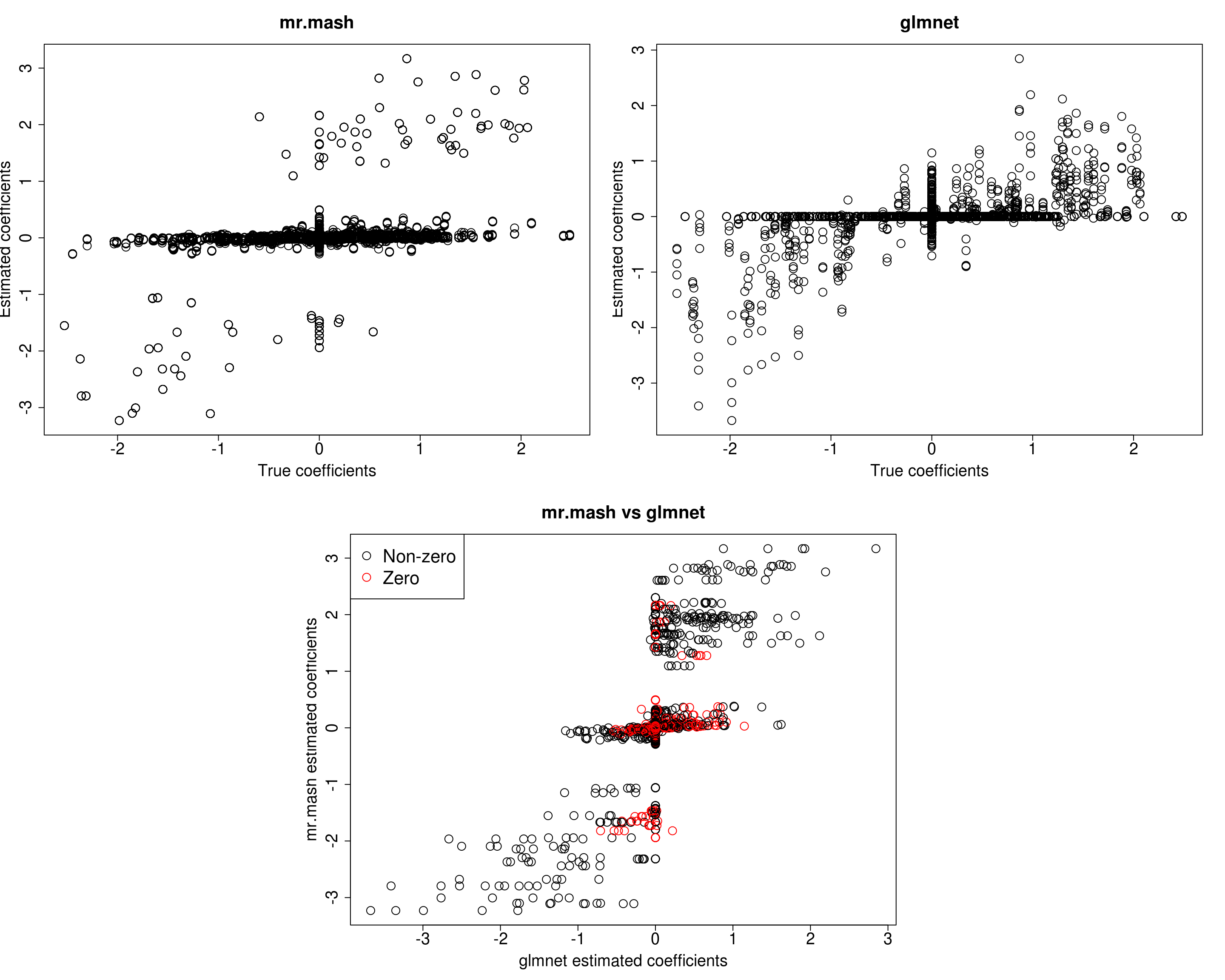
print("Prediction performance with glmnet")[1] "Prediction performance with glmnet"compute_accuracy(Ytest, Yhat_test_glmnet)$bias
[1] 0.8512846 1.1180041 1.2579560 1.0588456 0.9750071
$r2
[1] 0.08147787 0.13022180 0.14289736 0.10333887 0.09575056
$mse
[1] 545.7879 564.5279 615.7842 519.2563 549.6524print("Prediction performance with mr.mash")[1] "Prediction performance with mr.mash"compute_accuracy(Ytest, Yhat_test_mrmash_fixV)$bias
[1] 0.4388856 0.5346376 0.5651601 0.4447900 0.4799520
$r2
[1] 0.09424586 0.12724880 0.13040179 0.09928547 0.11030759
$mse
[1] 627.9131 627.6031 675.0825 610.6552 619.2527Prediction performance looks worse in terms of MSE and \(r^2\) while bias, although still off, is closer to 1. However, looking at the plots of the coefficients, we can see that many coefficients are no longer overshrunk. Let’s see what happens if we initialize V to the truth but then we update it.
###Fit mr.mash
fit_mrmash_initV <- mr.mash(Xtrain, Ytrain, S0, tol=1e-2, convergence_criterion="ELBO", update_w0=TRUE,
                     update_w0_method="EM", compute_ELBO=TRUE, standardize=TRUE, verbose=FALSE, update_V=TRUE,
                     mu1_init = Bhat_glmnet, w0_threshold=1e-8, V=out$V)
Processing the inputs... Done!
Fitting the optimization algorithm... Done!
Processing the outputs... Done!
mr.mash successfully executed in 3.177592 minutes!Yhat_test_mrmash_initV <- predict(fit_mrmash_initV, Xtest)layout(matrix(c(1, 1, 2, 2,
1, 1, 2, 2,
0, 3, 3, 0,
0, 3, 3, 0), 4, 4, byrow = TRUE))
###Plot estimated vs true coeffcients
##mr.mash
plot(out$B, fit_mrmash_initV$mu1, main="mr.mash", xlab="True coefficients", ylab="Estimated coefficients",
cex=2, cex.lab=1.8, cex.main=2, cex.axis=1.8)
##glmnet
plot(out$B, Bhat_glmnet, main="glmnet", xlab="True coefficients", ylab="Estimated coefficients",
cex=2, cex.lab=1.8, cex.main=2, cex.axis=1.8)
###Plot mr.mash vs glmnet estimated coeffcients
colorz <- matrix("black", nrow=p, ncol=r)
zeros <- apply(out$B, 2, function(x) x==0)
for(i in 1:ncol(colorz)){
colorz[zeros[, i], i] <- "red"
}
plot(Bhat_glmnet, fit_mrmash_initV$mu1, main="mr.mash vs glmnet",
xlab="glmnet estimated coefficients", ylab="mr.mash estimated coefficients",
col=colorz, cex=2, cex.lab=1.8, cex.main=2, cex.axis=1.8)
legend("topleft",
legend = c("Non-zero", "Zero"),
col = c("black", "red"),
pch = c(1, 1),
horiz = FALSE,
cex=2) 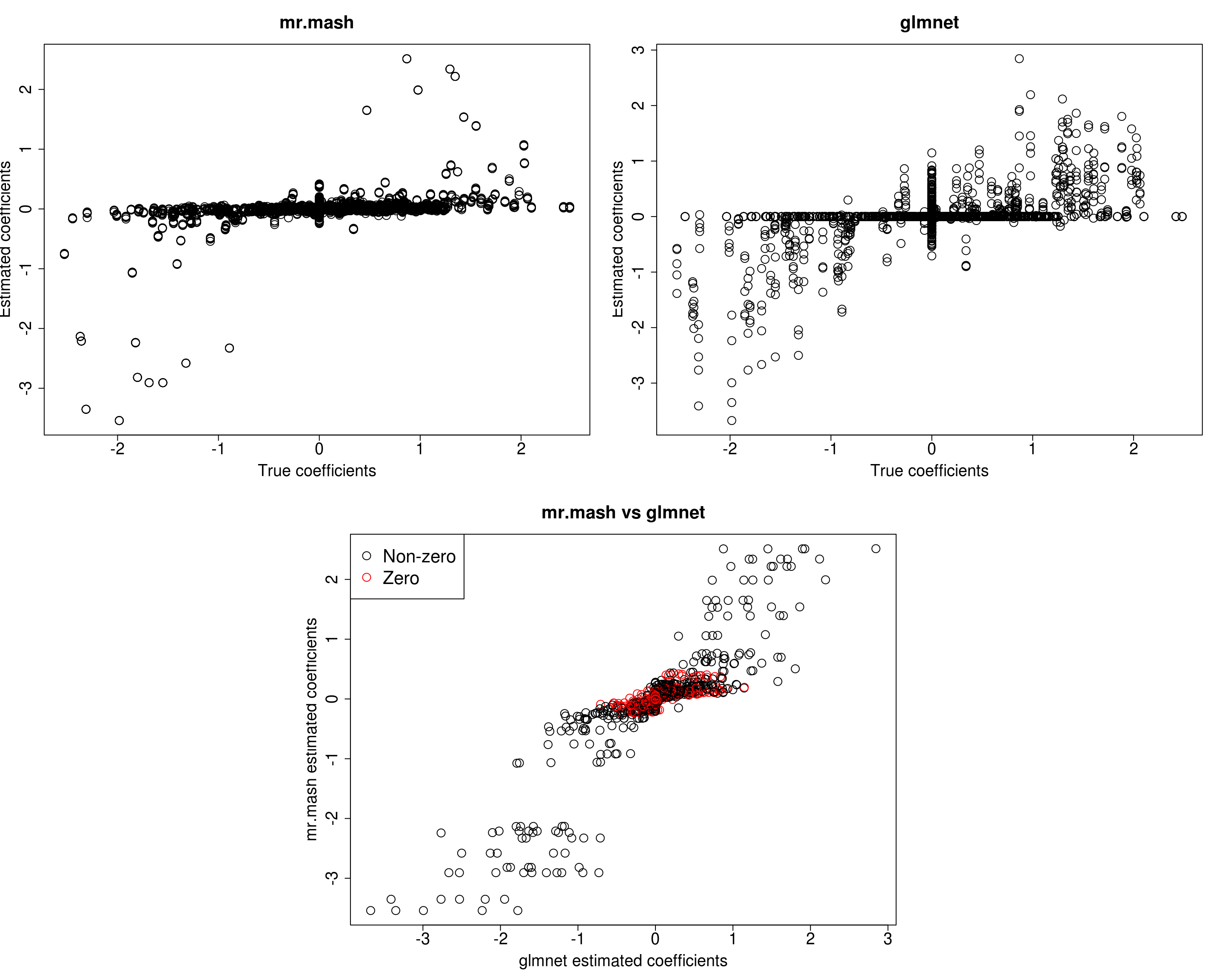
print("Prediction performance with glmnet")[1] "Prediction performance with glmnet"compute_accuracy(Ytest, Yhat_test_glmnet)$bias
[1] 0.8512846 1.1180041 1.2579560 1.0588456 0.9750071
$r2
[1] 0.08147787 0.13022180 0.14289736 0.10333887 0.09575056
$mse
[1] 545.7879 564.5279 615.7842 519.2563 549.6524print("Prediction performance with mr.mash")[1] "Prediction performance with mr.mash"compute_accuracy(Ytest, Yhat_test_mrmash_initV)$bias
[1] 0.6517158 0.9183659 0.9411075 0.7708241 0.7797849
$r2
[1] 0.06605841 0.11927623 0.11548872 0.09434182 0.09203971
$mse
[1] 564.6280 571.3815 631.5556 529.2132 556.3446print("True V (full data)")[1] "True V (full data)"out$V [,1] [,2] [,3] [,4] [,5]
[1,] 318.8014 0.0000 0.0000 0.0000 0.0000
[2,] 0.0000 318.8014 0.0000 0.0000 0.0000
[3,] 0.0000 0.0000 318.8014 0.0000 0.0000
[4,] 0.0000 0.0000 0.0000 318.8014 0.0000
[5,] 0.0000 0.0000 0.0000 0.0000 318.8014print("Estimated V (training data)")[1] "Estimated V (training data)"fit_mrmash_initV$V Y1 Y2 Y3 Y4 Y5
Y1 490.0991 167.7206 160.6264 147.9331 173.9756
Y2 167.7206 526.2906 174.7637 151.7885 194.2077
Y3 160.6264 174.7637 431.1751 136.2462 183.0564
Y4 147.9331 151.7885 136.2462 379.9678 157.3929
Y5 173.9756 194.2077 183.0564 157.3929 527.2299Here, we can see that that initilizing the residual covariance to the truth leads to essentially the same solutions as using the default initialization method.
After modifying mr.mash, we can now update the residual covariance imposing a diagonal structure. Let’s see how that works.
###Fit mr.mash
fit_mrmash_diagV <- mr.mash(Xtrain, Ytrain, S0, tol=1e-2, convergence_criterion="ELBO", update_w0=TRUE,
                            update_w0_method="EM", compute_ELBO=TRUE, standardize=TRUE, verbose=FALSE, update_V=TRUE,
                            update_V_method="diagonal", mu1_init=Bhat_glmnet, w0_threshold=1e-8)
Processing the inputs... Done!
Fitting the optimization algorithm... Done!
Processing the outputs... Done!
mr.mash successfully executed in 2.899423 minutes!Yhat_test_mrmash_diagV <- predict(fit_mrmash_diagV, Xtest)layout(matrix(c(1, 1, 2, 2,
1, 1, 2, 2,
0, 3, 3, 0,
0, 3, 3, 0), 4, 4, byrow = TRUE))
###Plot estimated vs true coeffcients
##mr.mash
plot(out$B, fit_mrmash_diagV$mu1, main="mr.mash", xlab="True coefficients", ylab="Estimated coefficients",
cex=2, cex.lab=1.8, cex.main=2, cex.axis=1.8)
##glmnet
plot(out$B, Bhat_glmnet, main="glmnet", xlab="True coefficients", ylab="Estimated coefficients",
cex=2, cex.lab=1.8, cex.main=2, cex.axis=1.8)
###Plot mr.mash vs glmnet estimated coeffcients
colorz <- matrix("black", nrow=p, ncol=r)
zeros <- apply(out$B, 2, function(x) x==0)
for(i in 1:ncol(colorz)){
colorz[zeros[, i], i] <- "red"
}
plot(Bhat_glmnet, fit_mrmash_diagV$mu1, main="mr.mash vs glmnet",
xlab="glmnet estimated coefficients", ylab="mr.mash estimated coefficients",
col=colorz, cex=2, cex.lab=1.8, cex.main=2, cex.axis=1.8)
legend("topleft",
legend = c("Non-zero", "Zero"),
col = c("black", "red"),
pch = c(1, 1),
horiz = FALSE,
cex=2) 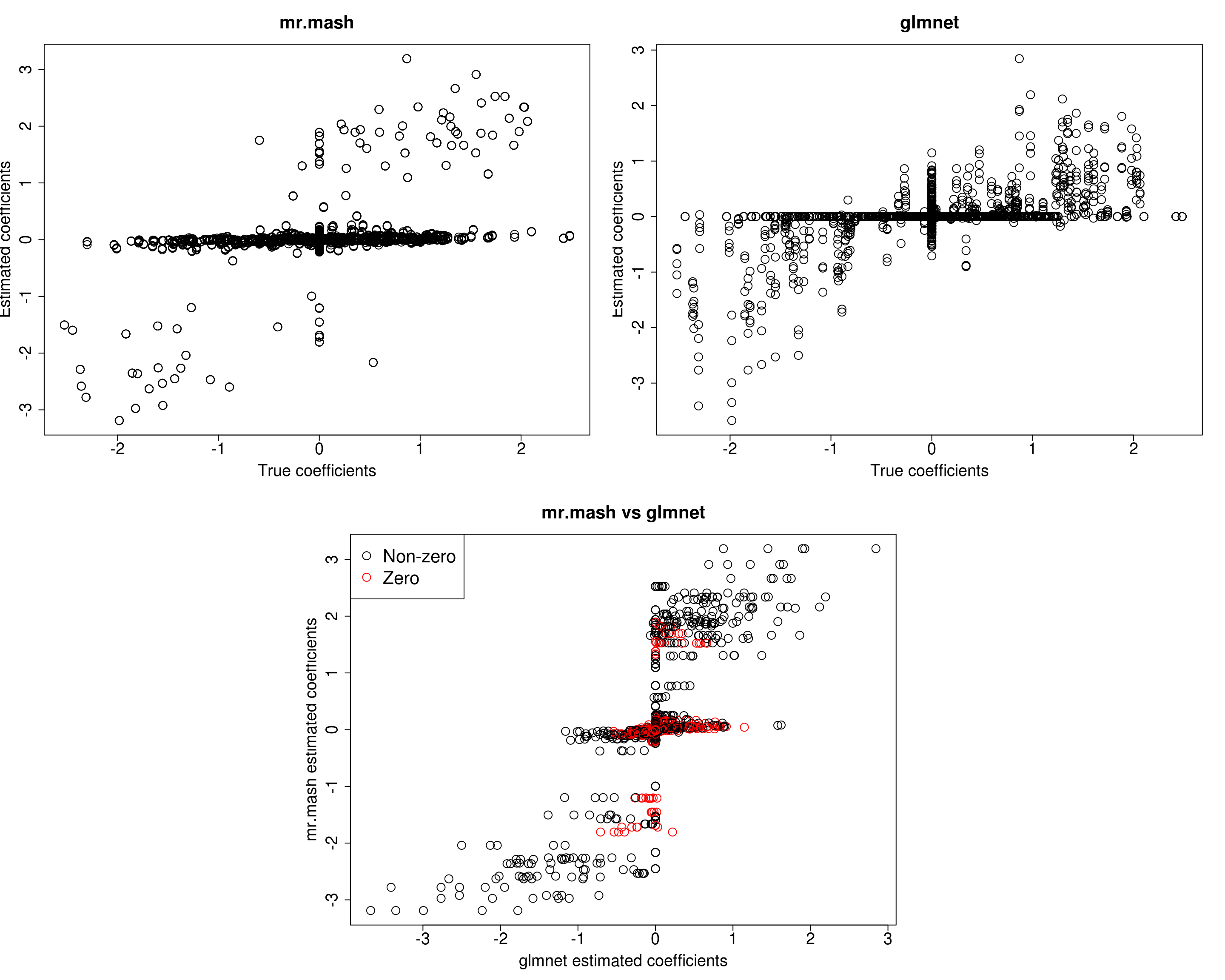
print("Prediction performance with glmnet")[1] "Prediction performance with glmnet"compute_accuracy(Ytest, Yhat_test_glmnet)$bias
[1] 0.8512846 1.1180041 1.2579560 1.0588456 0.9750071
$r2
[1] 0.08147787 0.13022180 0.14289736 0.10333887 0.09575056
$mse
[1] 545.7879 564.5279 615.7842 519.2563 549.6524print("Prediction performance with mr.mash")[1] "Prediction performance with mr.mash"compute_accuracy(Ytest, Yhat_test_mrmash_diagV)$bias
[1] 0.5055930 0.5973226 0.6661191 0.4961578 0.5509116
$r2
[1] 0.1171651 0.1491995 0.1697827 0.1156971 0.1358167
$mse
[1] 589.5178 595.1503 622.9059 580.9298 580.0254print("True V (full data)")[1] "True V (full data)"out$V [,1] [,2] [,3] [,4] [,5]
[1,] 318.8014 0.0000 0.0000 0.0000 0.0000
[2,] 0.0000 318.8014 0.0000 0.0000 0.0000
[3,] 0.0000 0.0000 318.8014 0.0000 0.0000
[4,] 0.0000 0.0000 0.0000 318.8014 0.0000
[5,] 0.0000 0.0000 0.0000 0.0000 318.8014print("Estimated V (training data)")[1] "Estimated V (training data)"fit_mrmash_diagV$V Y1 Y2 Y3 Y4 Y5
Y1 347.9812 0.0000 0.0000 0.0000 0.0000
Y2 0.0000 379.9561 0.0000 0.0000 0.0000
Y3 0.0000 0.0000 308.6972 0.0000 0.0000
Y4 0.0000 0.0000 0.0000 269.3813 0.0000
Y5 0.0000 0.0000 0.0000 0.0000 376.9686Although the estimated residual covariance is much closer to the truth and now many coefficients are not overshrunk, prediction performance is still poor. Another possibility is that overshrinking of coefficients happens because the mixture weights are poorly initialized. Let’s now try to initialize the mixture weights to the truth.
###Fit mr.mash
w0 <- rep(0, length(S0))
w0[c(104, 111)] <- c(0.5, 0.5)
fit_mrmash_diagV_initw0 <- mr.mash(Xtrain, Ytrain, S0, w0=w0, tol=1e-2, convergence_criterion="ELBO", update_w0=TRUE,
                                   update_w0_method="EM", compute_ELBO=TRUE, standardize=TRUE, verbose=FALSE, update_V=TRUE,
                                   update_V_method="diagonal", mu1_init=Bhat_glmnet, w0_threshold=1e-8)
Processing the inputs... Done!
Fitting the optimization algorithm... Done!
Processing the outputs... Done!
mr.mash successfully executed in 0.3866981 minutes!Yhat_test_mrmash_diagV_initw0 <- predict(fit_mrmash_diagV_initw0, Xtest)layout(matrix(c(1, 1, 2, 2,
1, 1, 2, 2,
0, 3, 3, 0,
0, 3, 3, 0), 4, 4, byrow = TRUE))
###Plot estimated vs true coeffcients
##mr.mash
plot(out$B, fit_mrmash_diagV_initw0$mu1, main="mr.mash", xlab="True coefficients", ylab="Estimated coefficients",
cex=2, cex.lab=1.8, cex.main=2, cex.axis=1.8)
##glmnet
plot(out$B, Bhat_glmnet, main="glmnet", xlab="True coefficients", ylab="Estimated coefficients",
cex=2, cex.lab=1.8, cex.main=2, cex.axis=1.8)
###Plot mr.mash vs glmnet estimated coeffcients
colorz <- matrix("black", nrow=p, ncol=r)
zeros <- apply(out$B, 2, function(x) x==0)
for(i in 1:ncol(colorz)){
colorz[zeros[, i], i] <- "red"
}
plot(Bhat_glmnet, fit_mrmash_diagV_initw0$mu1, main="mr.mash vs glmnet",
xlab="glmnet estimated coefficients", ylab="mr.mash estimated coefficients",
col=colorz, cex=2, cex.lab=1.8, cex.main=2, cex.axis=1.8)
legend("topleft",
legend = c("Non-zero", "Zero"),
col = c("black", "red"),
pch = c(1, 1),
horiz = FALSE,
cex=2) 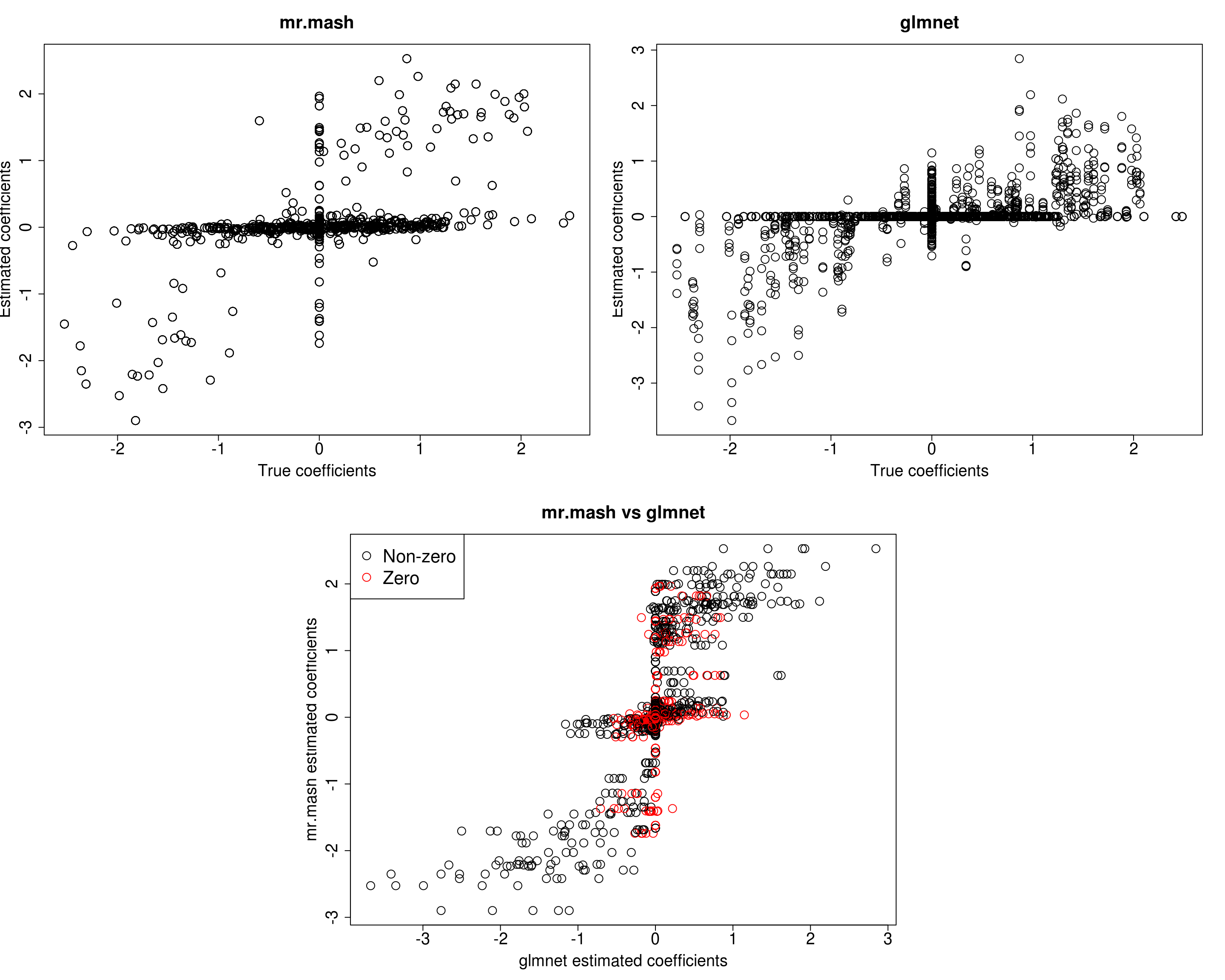
print("Prediction performance with glmnet")[1] "Prediction performance with glmnet"compute_accuracy(Ytest, Yhat_test_glmnet)$bias
[1] 0.8512846 1.1180041 1.2579560 1.0588456 0.9750071
$r2
[1] 0.08147787 0.13022180 0.14289736 0.10333887 0.09575056
$mse
[1] 545.7879 564.5279 615.7842 519.2563 549.6524print("Prediction performance with mr.mash")[1] "Prediction performance with mr.mash"compute_accuracy(Ytest, Yhat_test_mrmash_diagV_initw0)$bias
[1] 0.5847326 0.7040007 0.7906296 0.6201078 0.6626815
$r2
[1] 0.1073869 0.1426389 0.1636928 0.1238145 0.1345438
$mse
[1] 560.9732 571.7148 604.8914 534.0159 547.0646print("True V (full data)")[1] "True V (full data)"out$V [,1] [,2] [,3] [,4] [,5]
[1,] 318.8014 0.0000 0.0000 0.0000 0.0000
[2,] 0.0000 318.8014 0.0000 0.0000 0.0000
[3,] 0.0000 0.0000 318.8014 0.0000 0.0000
[4,] 0.0000 0.0000 0.0000 318.8014 0.0000
[5,] 0.0000 0.0000 0.0000 0.0000 318.8014print("Estimated V (training data)")[1] "Estimated V (training data)"fit_mrmash_diagV_initw0$V Y1 Y2 Y3 Y4 Y5
Y1 346.3538 0.0000 0.0000 0.000 0.0000
Y2 0.0000 397.1369 0.0000 0.000 0.0000
Y3 0.0000 0.0000 312.6765 0.000 0.0000
Y4 0.0000 0.0000 0.0000 270.874 0.0000
Y5 0.0000 0.0000 0.0000 0.000 383.9086Now, prediction performance is better. Next, let’s try to fix the mixture weights to the truth.
###Fit mr.mash
fit_mrmash_diagV_truew0 <- mr.mash(Xtrain, Ytrain, S0, w0=w0, tol=1e-2, convergence_criterion="ELBO", update_w0=FALSE,
                                    update_w0_method="EM", compute_ELBO=TRUE, standardize=TRUE, verbose=FALSE, update_V=TRUE,
                                    update_V_method="diagonal", mu1_init=Bhat_glmnet, w0_threshold=1e-8)
Processing the inputs... Done!
Fitting the optimization algorithm... Done!
Processing the outputs... Done!
mr.mash successfully executed in 0.8566629 minutes!Yhat_test_mrmash_diagV_truew0 <- predict(fit_mrmash_diagV_truew0, Xtest)layout(matrix(c(1, 1, 2, 2,
1, 1, 2, 2,
0, 3, 3, 0,
0, 3, 3, 0), 4, 4, byrow = TRUE))
###Plot estimated vs true coeffcients
##mr.mash
plot(out$B, fit_mrmash_diagV_truew0$mu1, main="mr.mash", xlab="True coefficients", ylab="Estimated coefficients",
cex=2, cex.lab=1.8, cex.main=2, cex.axis=1.8)
##glmnet
plot(out$B, Bhat_glmnet, main="glmnet", xlab="True coefficients", ylab="Estimated coefficients",
cex=2, cex.lab=1.8, cex.main=2, cex.axis=1.8)
###Plot mr.mash vs glmnet estimated coeffcients
colorz <- matrix("black", nrow=p, ncol=r)
zeros <- apply(out$B, 2, function(x) x==0)
for(i in 1:ncol(colorz)){
colorz[zeros[, i], i] <- "red"
}
plot(Bhat_glmnet, fit_mrmash_diagV_truew0$mu1, main="mr.mash vs glmnet",
xlab="glmnet estimated coefficients", ylab="mr.mash estimated coefficients",
col=colorz, cex=2, cex.lab=1.8, cex.main=2, cex.axis=1.8)
legend("topleft",
legend = c("Non-zero", "Zero"),
col = c("black", "red"),
pch = c(1, 1),
horiz = FALSE,
cex=2) 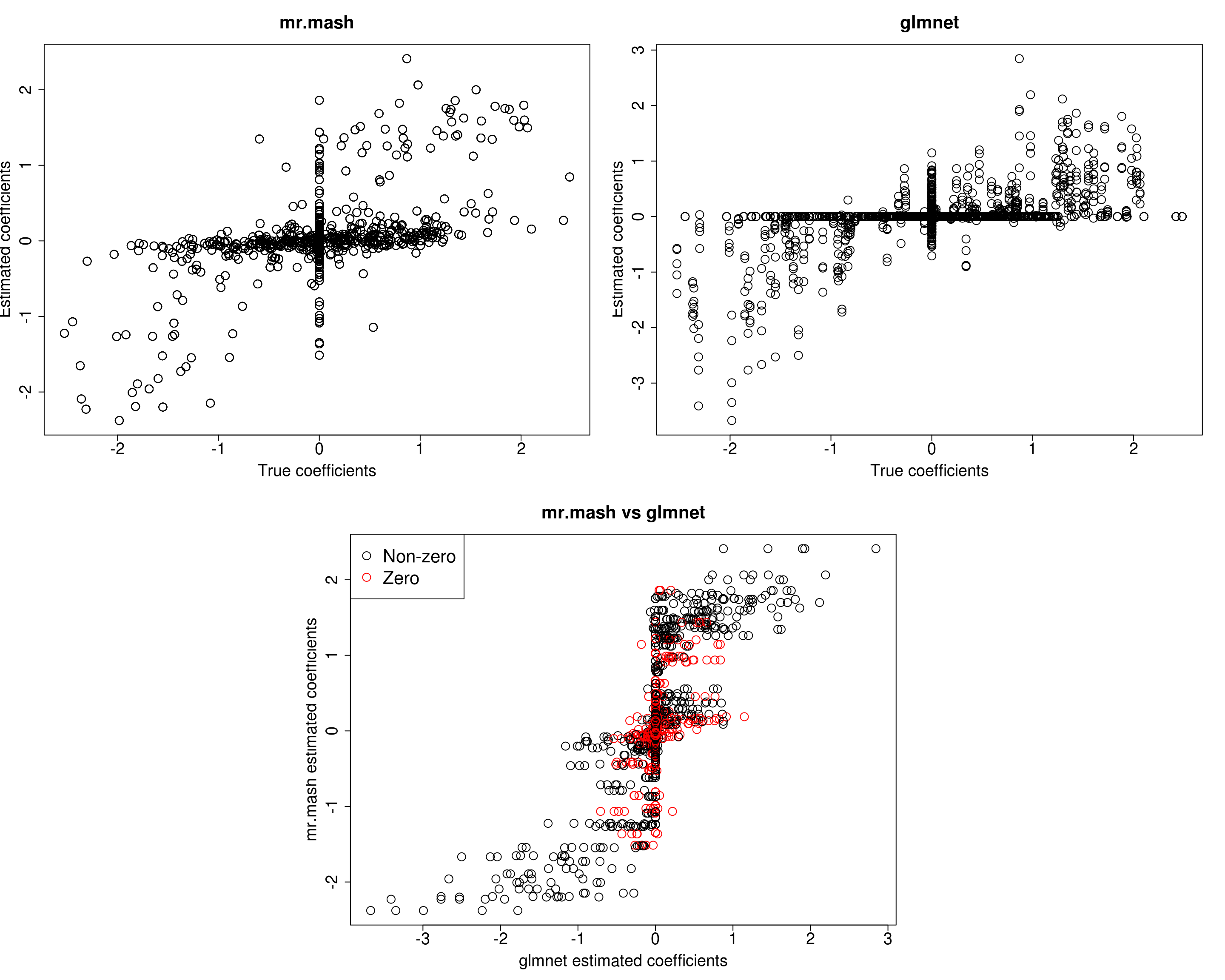
print("Prediction performance with glmnet")[1] "Prediction performance with glmnet"compute_accuracy(Ytest, Yhat_test_glmnet)$bias
[1] 0.8512846 1.1180041 1.2579560 1.0588456 0.9750071
$r2
[1] 0.08147787 0.13022180 0.14289736 0.10333887 0.09575056
$mse
[1] 545.7879 564.5279 615.7842 519.2563 549.6524print("Prediction performance with mr.mash")[1] "Prediction performance with mr.mash"compute_accuracy(Ytest, Yhat_test_mrmash_diagV_truew0)$bias
[1] 0.7213450 0.8576250 0.9273799 0.7328750 0.7946515
$r2
[1] 0.1438929 0.1863817 0.1982966 0.1522697 0.1703428
$mse
[1] 519.8999 530.0643 572.4096 502.0776 510.8810print("True V (full data)")[1] "True V (full data)"out$V [,1] [,2] [,3] [,4] [,5]
[1,] 318.8014 0.0000 0.0000 0.0000 0.0000
[2,] 0.0000 318.8014 0.0000 0.0000 0.0000
[3,] 0.0000 0.0000 318.8014 0.0000 0.0000
[4,] 0.0000 0.0000 0.0000 318.8014 0.0000
[5,] 0.0000 0.0000 0.0000 0.0000 318.8014print("Estimated V (training data)")[1] "Estimated V (training data)"fit_mrmash_diagV_truew0$V Y1 Y2 Y3 Y4 Y5
Y1 350.8131 0.0000 0.0000 0.0000 0.0000
Y2 0.0000 398.0888 0.0000 0.0000 0.0000
Y3 0.0000 0.0000 312.0516 0.0000 0.0000
Y4 0.0000 0.0000 0.0000 277.4814 0.0000
Y5 0.0000 0.0000 0.0000 0.0000 383.0856Prediction accuracy is now good and better than group-lasso. Finally, let’s fix both the residual covariance and mixture weights to the truth.
###Fit mr.mash
fit_mrmash_trueV_truew0 <- mr.mash(Xtrain, Ytrain, S0, w0=w0, tol=1e-2, convergence_criterion="ELBO", update_w0=FALSE,
                                    update_w0_method="EM", compute_ELBO=TRUE, standardize=TRUE, verbose=FALSE, update_V=FALSE,
                                    update_V_method="diagonal", mu1_init=Bhat_glmnet, w0_threshold=1e-8, V=out$V)
Processing the inputs... Done!
Fitting the optimization algorithm... Done!
Processing the outputs... Done!
mr.mash successfully executed in 1.862052 minutes!Yhat_test_mrmash_trueV_truew0 <- predict(fit_mrmash_trueV_truew0, Xtest)layout(matrix(c(1, 1, 2, 2,
1, 1, 2, 2,
0, 3, 3, 0,
0, 3, 3, 0), 4, 4, byrow = TRUE))
###Plot estimated vs true coeffcients
##mr.mash
plot(out$B, fit_mrmash_trueV_truew0$mu1, main="mr.mash", xlab="True coefficients", ylab="Estimated coefficients",
cex=2, cex.lab=1.8, cex.main=2, cex.axis=1.8)
##glmnet
plot(out$B, Bhat_glmnet, main="glmnet", xlab="True coefficients", ylab="Estimated coefficients",
cex=2, cex.lab=1.8, cex.main=2, cex.axis=1.8)
###Plot mr.mash vs glmnet estimated coeffcients
colorz <- matrix("black", nrow=p, ncol=r)
zeros <- apply(out$B, 2, function(x) x==0)
for(i in 1:ncol(colorz)){
colorz[zeros[, i], i] <- "red"
}
plot(Bhat_glmnet, fit_mrmash_trueV_truew0$mu1, main="mr.mash vs glmnet",
xlab="glmnet estimated coefficients", ylab="mr.mash estimated coefficients",
col=colorz, cex=2, cex.lab=1.8, cex.main=2, cex.axis=1.8)
legend("topleft",
legend = c("Non-zero", "Zero"),
col = c("black", "red"),
pch = c(1, 1),
horiz = FALSE,
cex=2) 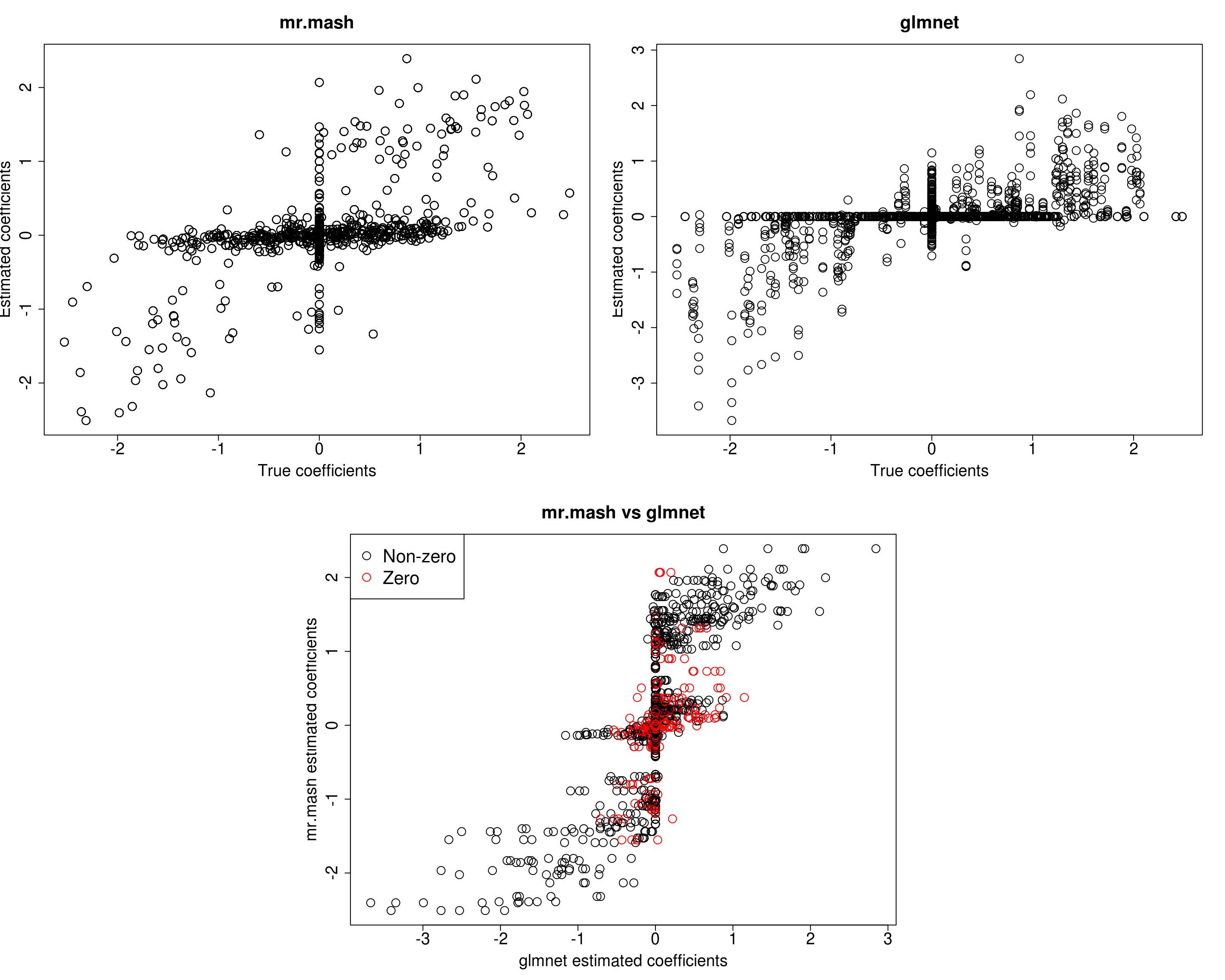
print("Prediction performance with glmnet")[1] "Prediction performance with glmnet"compute_accuracy(Ytest, Yhat_test_glmnet)$bias
[1] 0.8512846 1.1180041 1.2579560 1.0588456 0.9750071
$r2
[1] 0.08147787 0.13022180 0.14289736 0.10333887 0.09575056
$mse
[1] 545.7879 564.5279 615.7842 519.2563 549.6524print("Prediction performance with mr.mash")[1] "Prediction performance with mr.mash"compute_accuracy(Ytest, Yhat_test_mrmash_trueV_truew0)$bias
[1] 0.7072783 0.8323298 0.8531695 0.6922553 0.7646095
$r2
[1] 0.1533563 0.1946108 0.1860537 0.1506101 0.1748307
$mse
[1] 517.1990 526.8574 584.6708 508.8264 511.4591Not surprisingly we now achieve the best accuracy of all models.
However, looking at ELBO for all the models fitted so far reveals something interesting. The models that provide the best prediction performance in the test set are those with smaller ELBO, and viceversa. My intuition is that the largest ELBO is due to those models having more free parameters (since the include updating the weights and V with no structure imposed).
print(paste("Update w0, update V:", fit_mrmash$ELBO))[1] "Update w0, update V: -11175.3716018461"print(paste("Update w0, fix V to the truth:", fit_mrmash_fixV$ELBO))[1] "Update w0, fix V to the truth: -11238.0171099136"print(paste("Update w0, update V initializing it to the truth:", fit_mrmash_initV$ELBO))[1] "Update w0, update V initializing it to the truth: -11175.3730696164"print(paste("Update w0, update V imposing a diagonal structure:", fit_mrmash_diagV$ELBO))[1] "Update w0, update V imposing a diagonal structure: -11229.4169361434"print(paste("Update w0 initializing them to the truth, update V imposing a diagonal structure:", fit_mrmash_diagV_initw0$ELBO))[1] "Update w0 initializing them to the truth, update V imposing a diagonal structure: -11243.3199315825"print(paste("Fix w0 to the truth, update V imposing a diagonal structure:", fit_mrmash_diagV_truew0$ELBO))[1] "Fix w0 to the truth, update V imposing a diagonal structure: -11317.2706086721"print(paste("Fix w0 and V to the truth:", fit_mrmash_trueV_truew0$ELBO))[1] "Fix w0 and V to the truth: -11326.6122079057"Sparser scenario
For comparison let’s try to repeat the analysis above (updating V) on a sparser scenario, i.e., p_causal=50.
###Set parameters
n <- 1000
p <- 1000
p_causal <- 50
r <- 5
r_causal <- r
pve <- 0.5
B_cor <- 1
X_cor <- 0
V_cor <- 0

###Simulate V, B, X and Y
out50 <- mr.mash.alpha:::simulate_mr_mash_data(n, p, p_causal, r, r_causal=r, intercepts = rep(1, r),
                                             pve=pve, B_cor=B_cor, B_scale=0.9, X_cor=X_cor, X_scale=0.8, V_cor=V_cor)

colnames(out50$Y) <- paste0("Y", seq(1, r))
rownames(out50$Y) <- paste0("N", seq(1, n))
colnames(out50$X) <- paste0("X", seq(1, p))
rownames(out50$X) <- paste0("N", seq(1, n))

###Split the data in training and test sets
test_set50 <- sort(sample(x=c(1:n), size=round(n*0.5), replace=FALSE))
Ytrain50 <- out50$Y[-test_set50, ]
Xtrain50 <- out50$X[-test_set50, ]
Ytest50 <- out50$Y[test_set50, ]
Xtest50 <- out50$X[test_set50, ]

###Fit group-lasso
cvfit_glmnet50 <- cv.glmnet(x=Xtrain50, y=Ytrain50, family="mgaussian", alpha=1)
coeff_glmnet50 <- coef(cvfit_glmnet50, s="lambda.min")
Bhat_glmnet50 <- matrix(as.numeric(NA), nrow=p, ncol=r)
ahat_glmnet50 <- vector("numeric", r)
for(i in 1:length(coeff_glmnet50)){
  Bhat_glmnet50[, i] <- as.vector(coeff_glmnet50[[i]])[-1]
  ahat_glmnet50[i] <- as.vector(coeff_glmnet50[[i]])[1]
}
Yhat_test_glmnet50 <- drop(predict(cvfit_glmnet50, newx=Xtest50, s="lambda.min"))

###Fit mr.mash
fit_mrmash50 <- mr.mash(Xtrain50, Ytrain50, S0, tol=1e-2, convergence_criterion="ELBO", update_w0=TRUE,
                     update_w0_method="EM", compute_ELBO=TRUE, standardize=TRUE, verbose=FALSE, update_V=TRUE,
                     mu1_init = Bhat_glmnet50, w0_threshold=1e-8)
Processing the inputs... Done!
Fitting the optimization algorithm... Done!
Processing the outputs... Done!
mr.mash successfully executed in 0.9788831 minutes!Yhat_test_mrmash50 <- predict(fit_mrmash50, Xtest50)layout(matrix(c(1, 1, 2, 2,
1, 1, 2, 2,
0, 3, 3, 0,
0, 3, 3, 0), 4, 4, byrow = TRUE))
###Plot estimated vs true coeffcients
##mr.mash
plot(out50$B, fit_mrmash50$mu1, main="mr.mash", xlab="True coefficients", ylab="Estimated coefficients",
cex=2, cex.lab=1.8, cex.main=2, cex.axis=1.8)
##glmnet
plot(out50$B, Bhat_glmnet50, main="glmnet", xlab="True coefficients", ylab="Estimated coefficients",
cex=2, cex.lab=1.8, cex.main=2, cex.axis=1.8)
###Plot mr.mash vs glmnet estimated coeffcients
colorz <- matrix("black", nrow=p, ncol=r)
zeros <- apply(out50$B, 2, function(x) x==0)
for(i in 1:ncol(colorz)){
colorz[zeros[, i], i] <- "red"
}
plot(Bhat_glmnet50, fit_mrmash50$mu1, main="mr.mash vs glmnet",
xlab="glmnet estimated coefficients", ylab="mr.mash estimated coefficients",
col=colorz, cex=2, cex.lab=1.8, cex.main=2, cex.axis=1.8)
legend("topleft",
legend = c("Non-zero", "Zero"),
col = c("black", "red"),
pch = c(1, 1),
horiz = FALSE,
cex=2) 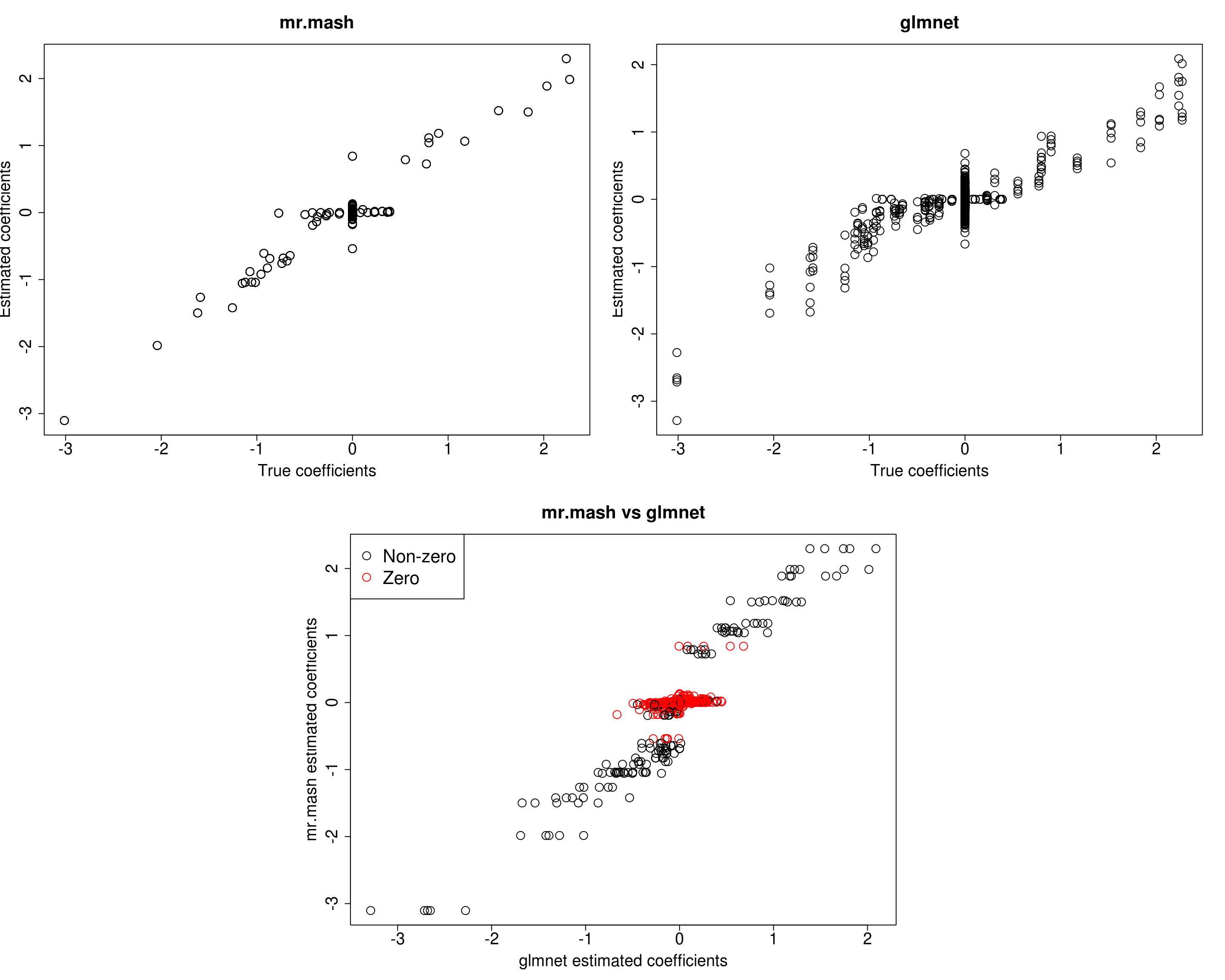
print("Prediction performance with glmnet")[1] "Prediction performance with glmnet"compute_accuracy(Ytest50, Yhat_test_glmnet50)$bias
[1] 1.199362 1.379444 1.076210 1.295043 1.261338
$r2
[1] 0.4138042 0.4650768 0.3838995 0.4621230 0.3903651
$mse
[1] 55.85811 58.97457 58.10302 54.64713 64.96945print("Prediction performance with mr.mash")[1] "Prediction performance with mr.mash"compute_accuracy(Ytest50, Yhat_test_mrmash50)$bias
[1] 0.9598673 1.0442544 0.9326388 1.0081957 0.9972526
$r2
[1] 0.4915822 0.5269943 0.4646516 0.5201747 0.4770788
$mse
[1] 47.60989 49.10529 50.46953 46.69598 54.35184print("True V (full data)")[1] "True V (full data)"out50$V [,1] [,2] [,3] [,4] [,5]
[1,] 48.70994 0.00000 0.00000 0.00000 0.00000
[2,] 0.00000 48.70994 0.00000 0.00000 0.00000
[3,] 0.00000 0.00000 48.70994 0.00000 0.00000
[4,] 0.00000 0.00000 0.00000 48.70994 0.00000
[5,] 0.00000 0.00000 0.00000 0.00000 48.70994print("Estimated V (training data)")[1] "Estimated V (training data)"fit_mrmash50$V Y1 Y2 Y3 Y4 Y5
Y1 47.14100703 3.499271 1.8974135 0.6745678 -0.08287119
Y2 3.49927140 48.523627 -2.3529618 2.7666402 1.33756992
Y3 1.89741348 -2.352962 49.5967297 4.4538398 -0.95114634
Y4 0.67456782 2.766640 4.4538398 54.2393501 -0.89130437
Y5 -0.08287119 1.337570 -0.9511463 -0.8913044 51.07249272The results of this simulation look very good in terms of prediction performance, estimation of the coefficients, and estimation of the residual covariance.
Dense scenario (fewer variables)
Just as an additional test let’s now try to maintain the same signal-to-noise ratio as the first simulation but with fewer total variables, i.e., p=500 and p_causal=250.
###Set parameters
n <- 1000
p <- 500
p_causal <- 250
r <- 5
r_causal <- r
pve <- 0.5
B_cor <- 1
X_cor <- 0
V_cor <- 0

###Simulate V, B, X and Y
out500 <- mr.mash.alpha:::simulate_mr_mash_data(n, p, p_causal, r, r_causal=r, intercepts = rep(1, r),
                                             pve=pve, B_cor=B_cor, B_scale=0.9, X_cor=X_cor, X_scale=0.8, V_cor=V_cor)

colnames(out500$Y) <- paste0("Y", seq(1, r))
rownames(out500$Y) <- paste0("N", seq(1, n))
colnames(out500$X) <- paste0("X", seq(1, p))
rownames(out500$X) <- paste0("N", seq(1, n))

###Split the data in training and test sets
test_set500 <- sort(sample(x=c(1:n), size=round(n*0.5), replace=FALSE))
Ytrain500 <- out500$Y[-test_set500, ]
Xtrain500 <- out500$X[-test_set500, ]
Ytest500 <- out500$Y[test_set500, ]
Xtest500 <- out500$X[test_set500, ]

###Fit group-lasso
cvfit_glmnet500 <- cv.glmnet(x=Xtrain500, y=Ytrain500, family="mgaussian", alpha=1)
coeff_glmnet500 <- coef(cvfit_glmnet500, s="lambda.min")
Bhat_glmnet500 <- matrix(as.numeric(NA), nrow=p, ncol=r)
ahat_glmnet500 <- vector("numeric", r)
for(i in 1:length(coeff_glmnet500)){
  Bhat_glmnet500[, i] <- as.vector(coeff_glmnet500[[i]])[-1]
  ahat_glmnet500[i] <- as.vector(coeff_glmnet500[[i]])[1]
}
Yhat_test_glmnet500 <- drop(predict(cvfit_glmnet500, newx=Xtest500, s="lambda.min"))

###Fit mr.mash
fit_mrmash500 <- mr.mash(Xtrain500, Ytrain500, S0, tol=1e-2, convergence_criterion="ELBO", update_w0=TRUE,
                     update_w0_method="EM", compute_ELBO=TRUE, standardize=TRUE, verbose=FALSE, update_V=TRUE,
                     mu1_init = Bhat_glmnet500, w0_threshold=1e-8)
Processing the inputs... Done!
Fitting the optimization algorithm... Done!
Processing the outputs... Done!
mr.mash successfully executed in 1.08829 minutes!Yhat_test_mrmash500 <- predict(fit_mrmash500, Xtest500)layout(matrix(c(1, 1, 2, 2,
1, 1, 2, 2,
0, 3, 3, 0,
0, 3, 3, 0), 4, 4, byrow = TRUE))
###Plot estimated vs true coeffcients
##mr.mash
plot(out500$B, fit_mrmash500$mu1, main="mr.mash", xlab="True coefficients", ylab="Estimated coefficients",
cex=2, cex.lab=1.8, cex.main=2, cex.axis=1.8)
##glmnet
plot(out500$B, Bhat_glmnet500, main="glmnet", xlab="True coefficients", ylab="Estimated coefficients",
cex=2, cex.lab=1.8, cex.main=2, cex.axis=1.8)
###Plot mr.mash vs glmnet estimated coeffcients
colorz <- matrix("black", nrow=p, ncol=r)
zeros <- apply(out500$B, 2, function(x) x==0)
for(i in 1:ncol(colorz)){
colorz[zeros[, i], i] <- "red"
}
plot(Bhat_glmnet500, fit_mrmash500$mu1, main="mr.mash vs glmnet",
xlab="glmnet estimated coefficients", ylab="mr.mash estimated coefficients",
col=colorz, cex=2, cex.lab=1.8, cex.main=2, cex.axis=1.8)
legend("topleft",
legend = c("Non-zero", "Zero"),
col = c("black", "red"),
pch = c(1, 1),
horiz = FALSE,
cex=2) 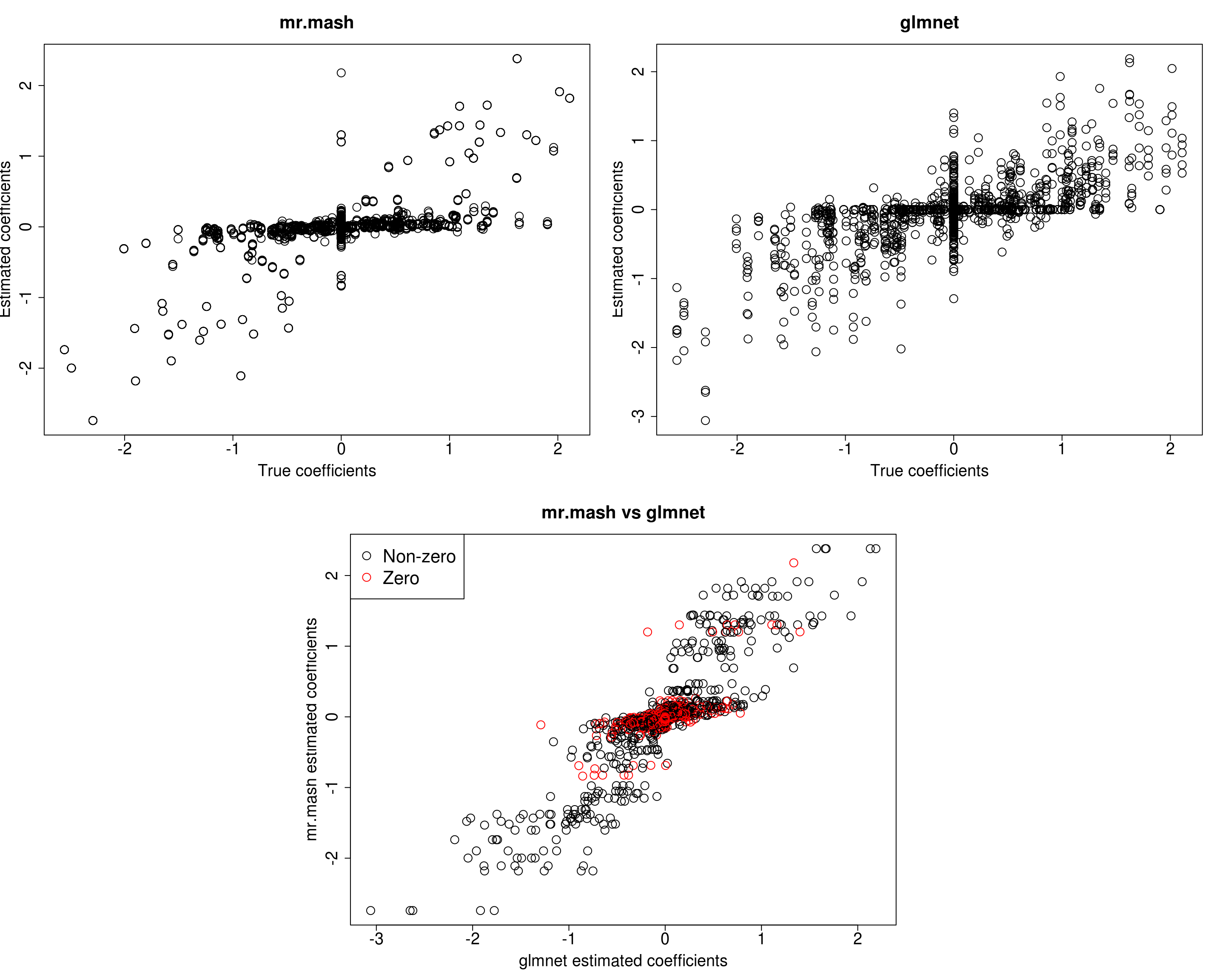
print("Prediction performance with glmnet")[1] "Prediction performance with glmnet"compute_accuracy(Ytest500, Yhat_test_glmnet500)$bias
[1] 1.1255548 1.1507096 1.2025003 1.1321183 0.9449982
$r2
[1] 0.2456096 0.2086680 0.2525343 0.2178140 0.2241591
$mse
[1] 243.5651 245.6349 248.0822 242.4490 213.1741print("Prediction performance with mr.mash")[1] "Prediction performance with mr.mash"compute_accuracy(Ytest500, Yhat_test_mrmash500)$bias
[1] 0.9242366 0.9082153 0.9863245 0.9116667 0.8504277
$r2
[1] 0.2367275 0.2421513 0.2639270 0.2373244 0.2482003
$mse
[1] 244.4928 233.5644 242.0282 236.2430 207.8620print("True V (full data)")[1] "True V (full data)"out500$V [,1] [,2] [,3] [,4] [,5]
[1,] 158.7435 0.0000 0.0000 0.0000 0.0000
[2,] 0.0000 158.7435 0.0000 0.0000 0.0000
[3,] 0.0000 0.0000 158.7435 0.0000 0.0000
[4,] 0.0000 0.0000 0.0000 158.7435 0.0000
[5,] 0.0000 0.0000 0.0000 0.0000 158.7435print("Estimated V (training data)")[1] "Estimated V (training data)"fit_mrmash500$V Y1 Y2 Y3 Y4 Y5
Y1 183.39698 32.589382 29.23365 29.286564 34.280134
Y2 32.58938 180.306943 32.29370 5.839094 7.604363
Y3 29.23365 32.293700 195.98299 26.927416 27.605103
Y4 29.28656 5.839094 26.92742 181.142905 27.707847
Y5 34.28013 7.604363 27.60510 27.707847 168.922558In this last simulation, we can see that mr.mash performs pretty well, even in a denser scenario with fewer variables.
sessionInfo()R version 3.5.1 (2018-07-02)
Platform: x86_64-pc-linux-gnu (64-bit)
Running under: Scientific Linux 7.4 (Nitrogen)
Matrix products: default
BLAS/LAPACK: /software/openblas-0.2.19-el7-x86_64/lib/libopenblas_haswellp-r0.2.19.so
locale:
[1] LC_CTYPE=en_US.UTF-8 LC_NUMERIC=C
[3] LC_TIME=en_US.UTF-8 LC_COLLATE=en_US.UTF-8
[5] LC_MONETARY=en_US.UTF-8 LC_MESSAGES=en_US.UTF-8
[7] LC_PAPER=en_US.UTF-8 LC_NAME=C
[9] LC_ADDRESS=C LC_TELEPHONE=C
[11] LC_MEASUREMENT=en_US.UTF-8 LC_IDENTIFICATION=C
attached base packages:
[1] stats graphics grDevices utils datasets methods base
other attached packages:
[1] glmnet_2.0-16 foreach_1.4.4 Matrix_1.2-15
[4] mr.mash.alpha_0.1-76
loaded via a namespace (and not attached):
[1] MBSP_1.0 Rcpp_1.0.4.6 compiler_3.5.1
[4] later_0.7.5 git2r_0.26.1 workflowr_1.6.1
[7] iterators_1.0.10 tools_3.5.1 digest_0.6.25
[10] evaluate_0.12 lattice_0.20-38 GIGrvg_0.5
[13] yaml_2.2.1 SparseM_1.77 mvtnorm_1.0-12
[16] coda_0.19-3 stringr_1.4.0 knitr_1.20
[19] fs_1.3.1 MatrixModels_0.4-1 rprojroot_1.3-2
[22] grid_3.5.1 glue_1.4.0 R6_2.4.1
[25] rmarkdown_1.10 mixsqp_0.3-43 irlba_2.3.3
[28] magrittr_1.5 whisker_0.3-2 codetools_0.2-15
[31] backports_1.1.5 promises_1.0.1 htmltools_0.3.6
[34] matrixStats_0.55.0 mcmc_0.9-6 MASS_7.3-51.1
[37] httpuv_1.4.5 quantreg_5.36 stringi_1.4.3
[40] MCMCpack_1.4-4