Dense case
Fabio Morgante
June 01, 2020
Last updated: 2020-06-01
Checks: 7 0
Knit directory: mr_mash_test/
This reproducible R Markdown analysis was created with workflowr (version 1.6.1). The Checks tab describes the reproducibility checks that were applied when the results were created. The Past versions tab lists the development history.
Great! Since the R Markdown file has been committed to the Git repository, you know the exact version of the code that produced these results.
Great job! The global environment was empty. Objects defined in the global environment can affect the analysis in your R Markdown file in unknown ways. For reproduciblity it’s best to always run the code in an empty environment.
The command set.seed(20200328) was run prior to running the code in the R Markdown file. Setting a seed ensures that any results that rely on randomness, e.g. subsampling or permutations, are reproducible.
Great job! Recording the operating system, R version, and package versions is critical for reproducibility.
Nice! There were no cached chunks for this analysis, so you can be confident that you successfully produced the results during this run.
Great job! Using relative paths to the files within your workflowr project makes it easier to run your code on other machines.
Great! You are using Git for version control. Tracking code development and connecting the code version to the results is critical for reproducibility.
The results in this page were generated with repository version ceda278. See the Past versions tab to see a history of the changes made to the R Markdown and HTML files.
Note that you need to be careful to ensure that all relevant files for the analysis have been committed to Git prior to generating the results (you can use wflow_publish or wflow_git_commit). workflowr only checks the R Markdown file, but you know if there are other scripts or data files that it depends on. Below is the status of the Git repository when the results were generated:
Ignored files:
    Ignored:    .sos/
    Ignored:    code/fit_mr_mash.66662433.err
    Ignored:    code/fit_mr_mash.66662433.out
    Ignored:    dsc/.sos/
    Ignored:    dsc/outfiles/
    Ignored:    output/dsc.html
    Ignored:    output/dsc/
    Ignored:    output/dsc_05_18_20.html
    Ignored:    output/dsc_05_18_20/
    Ignored:    output/dsc_05_29_20.html
    Ignored:    output/dsc_05_29_20/
    Ignored:    output/dsc_OLD.html
    Ignored:    output/dsc_OLD/
    Ignored:    output/dsc_test.html
    Ignored:    output/dsc_test/

Untracked files:
    Untracked:  code/plot_test.R

Unstaged changes:
    Modified:   dsc/functions/fit_gflasso.R
    Modified:   dsc/midway2.yml
Note that any generated files, e.g. HTML, png, CSS, etc., are not included in this status report because it is ok for generated content to have uncommitted changes.
These are the previous versions of the repository in which changes were made to the R Markdown (analysis/dense_scenario_issue.Rmd) and HTML (docs/dense_scenario_issue.html) files. If you’ve configured a remote Git repository (see ?wflow_git_remote), click on the hyperlinks in the table below to view the files as they were in that past version.
| File | Version | Author | Date | Message |
|---|---|---|---|---|
| Rmd | ceda278 | fmorgante | 2020-06-01 | Add case study with dense scenario |
library(mr.mash.alpha)
library(glmnet)
Loading required package: MatrixLoading required package: foreachLoaded glmnet 2.0-16###Set options
options(stringsAsFactors = FALSE)
###Function to compute accuracy
compute_accuracy <- function(Y, Yhat) {
bias <- rep(as.numeric(NA), ncol(Y))
r2 <- rep(as.numeric(NA), ncol(Y))
mse <- rep(as.numeric(NA), ncol(Y))
for(i in 1:ncol(Y)){
fit <- lm(Y[, i] ~ Yhat[, i])
bias[i] <- coef(fit)[2]
r2[i] <- summary(fit)$r.squared
mse[i] <- mean((Y[, i] - Yhat[, i])^2)
}
return(list(bias=bias, r2=r2, mse=mse))
}Here we investigate why mr.mash does not perform as well in denser scenarios. Let’s simulate data with n=600, p=1,000, p_causal=500, r=5, r_causal=5, PVE=0.5, shared effects, independent predictors, and independent residuals. The models will be fitted to the training data (80% of the full data).
###Set seed
set.seed(123)

###Set parameters
n <- 600
p <- 1000
p_causal <- 500
r <- 5
r_causal <- r
pve <- 0.5
B_cor <- 1
X_cor <- 0
V_cor <- 0

###Simulate V, B, X and Y
out <- mr.mash.alpha:::simulate_mr_mash_data(n, p, p_causal, r, r_causal=r, intercepts = rep(1, r),
                                             pve=pve, B_cor=B_cor, B_scale=0.8, X_cor=X_cor, X_scale=0.8, V_cor=V_cor)

colnames(out$Y) <- paste0("Y", seq(1, r))
rownames(out$Y) <- paste0("N", seq(1, n))
colnames(out$X) <- paste0("X", seq(1, p))
rownames(out$X) <- paste0("N", seq(1, n))

###Split the data in training and test sets
test_set <- sort(sample(x=c(1:n), size=round(n*0.2), replace=FALSE))
Ytrain <- out$Y[-test_set, ]
Xtrain <- out$X[-test_set, ]
Ytest <- out$Y[test_set, ]
Xtest <- out$X[test_set, ]
We build the mixture prior as usual including zero matrix, identity matrix, rank-1 matrices, low, medium and high heterogeneity matrices, shared matrix, each scaled by a grid from 0.1 to 2.1 in steps of 0.2.
grid <- seq(0.1, 2.1, 0.2)
S0 <- mr.mash.alpha:::compute_cov_canonical(ncol(Ytrain), singletons=TRUE, hetgrid=c(0, 0.25, 0.5, 0.75, 1), grid, zeromat=TRUE)
We run glmnet with \(\alpha=1\) to obtain an inital estimate for the regression coefficients to provide to mr.mash, and for comparison.
###Fit group-lasso
cvfit_glmnet <- cv.glmnet(x=Xtrain, y=Ytrain, family="mgaussian", alpha=1)
coeff_glmnet <- coef(cvfit_glmnet, s="lambda.min")
Bhat_glmnet <- matrix(as.numeric(NA), nrow=p, ncol=r)
ahat_glmnet <- vector("numeric", r)
for(i in 1:length(coeff_glmnet)){
  Bhat_glmnet[, i] <- as.vector(coeff_glmnet[[i]])[-1]
  ahat_glmnet[i] <- as.vector(coeff_glmnet[[i]])[1]
}
Yhat_test_glmnet <- drop(predict(cvfit_glmnet, newx=Xtest, s="lambda.min"))
We run mr.mash with EM updates of the mixture weights, updating V, and initializing the regression coefficients with the estimates from glmnet.
###Fit mr.mash
fit_mrmash <- mr.mash(Xtrain, Ytrain, S0, tol=1e-2, convergence_criterion="ELBO", update_w0=TRUE,
                     update_w0_method="EM", compute_ELBO=TRUE, standardize=TRUE, verbose=FALSE, update_V=TRUE,
                     mu1_init = Bhat_glmnet, w0_threshold=1e-8)
Processing the inputs... Done!
Fitting the optimization algorithm... Done!
Processing the outputs... Done!
mr.mash successfully executed in 2.450516 minutes!Yhat_test_mrmash <- predict(fit_mrmash, Xtest)Let’s now compare the results.
layout(matrix(c(1, 1, 2, 2,
                1, 1, 2, 2,
                0, 3, 3, 0,
                0, 3, 3, 0), 4, 4, byrow = TRUE))

###Plot estimated vs true coeffcients
##mr.mash
plot(out$B, fit_mrmash$mu1, main="mr.mash", xlab="True coefficients", ylab="Estimated coefficients",
     cex=2, cex.lab=1.8, cex.main=2, cex.axis=1.8)
##glmnet
plot(out$B, Bhat_glmnet, main="glmnet", xlab="True coefficients", ylab="Estimated coefficients",
     cex=2, cex.lab=1.8, cex.main=2, cex.axis=1.8)

###Plot mr.mash vs glmnet estimated coeffcients
colorz <- matrix("black", nrow=p, ncol=r)
zeros <- apply(out$B, 2, function(x) x==0)
for(i in 1:ncol(colorz)){
  colorz[zeros[, i], i] <- "red"
}

plot(Bhat_glmnet, fit_mrmash$mu1, main="mr.mash vs glmnet",
     xlab="glmnet estimated coefficients", ylab="mr.mash estimated coefficients",
     col=colorz, cex=2, cex.lab=1.8, cex.main=2, cex.axis=1.8)
legend("topleft",
       legend = c("Non-zero", "Zero"),
       col = c("black", "red"),
       pch = c(1, 1),
       horiz = FALSE,
cex=2) 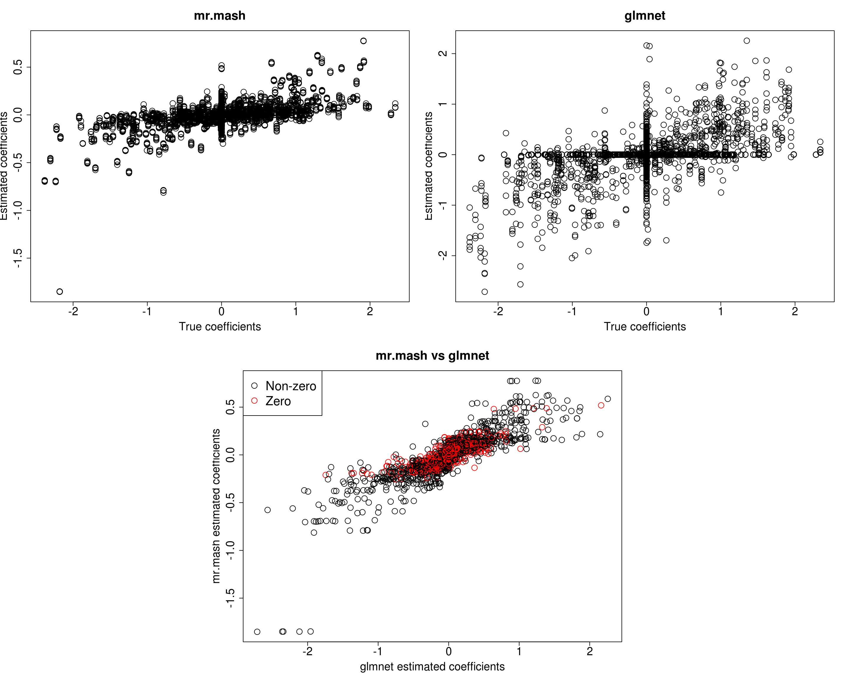
print("Prediction performance with glmnet")[1] "Prediction performance with glmnet"compute_accuracy(Ytest, Yhat_test_glmnet)$bias
[1] 0.7973441 0.7171240 1.1201318 0.9992656 0.9375002
$r2
[1] 0.12560024 0.10044653 0.14357016 0.13204939 0.09516285
$mse
[1] 446.4747 472.2412 509.8068 511.4644 642.4144print("Prediction performance with mr.mash")[1] "Prediction performance with mr.mash"compute_accuracy(Ytest, Yhat_test_mrmash)$bias
[1] 2.269604 2.196994 3.438804 2.832561 3.030053
$r2
[1] 0.1310534 0.1127552 0.2346756 0.1833728 0.1537069
$mse
[1] 460.6600 471.2208 525.7587 522.0806 649.4204print("True V (full data)")[1] "True V (full data)"out$V [,1] [,2] [,3] [,4] [,5]
[1,] 294.59 0.00 0.00 0.00 0.00
[2,] 0.00 294.59 0.00 0.00 0.00
[3,] 0.00 0.00 294.59 0.00 0.00
[4,] 0.00 0.00 0.00 294.59 0.00
[5,] 0.00 0.00 0.00 0.00 294.59print("Estimated V (training data)")[1] "Estimated V (training data)"fit_mrmash$V Y1 Y2 Y3 Y4 Y5
Y1 534.0861 241.6130 189.3974 175.6404 206.0833
Y2 241.6130 517.0130 217.6493 216.6763 227.4030
Y3 189.3974 217.6493 482.4770 224.0472 212.9069
Y4 175.6404 216.6763 224.0472 473.4047 190.4193
Y5 206.0833 227.4030 212.9069 190.4193 459.0911It looks mr.mash shrinks the coeffcients too much and the residual covariance is absorbing part of the effects. Let’s now try to fix the residual covariance to the truth (although it is going to be a little different since we are fitting the model to the training set only).
###Fit mr.mash
fit_mrmash_fixV <- mr.mash(Xtrain, Ytrain, S0, tol=1e-2, convergence_criterion="ELBO", update_w0=TRUE,
                     update_w0_method="EM", compute_ELBO=TRUE, standardize=TRUE, verbose=FALSE, update_V=FALSE,
                     mu1_init = Bhat_glmnet, w0_threshold=1e-8, V=out$V)
Processing the inputs... Done!
Fitting the optimization algorithm... Done!
Processing the outputs... Done!
mr.mash successfully executed in 3.078888 minutes!Yhat_test_mrmash_fixV <- predict(fit_mrmash_fixV, Xtest)Let’s compare the results again.
layout(matrix(c(1, 1, 2, 2,
                1, 1, 2, 2,
                0, 3, 3, 0,
                0, 3, 3, 0), 4, 4, byrow = TRUE))

###Plot estimated vs true coeffcients
##mr.mash
plot(out$B, fit_mrmash_fixV$mu1, main="mr.mash", xlab="True coefficients", ylab="Estimated coefficients",
     cex=2, cex.lab=1.8, cex.main=2, cex.axis=1.8)
##glmnet
plot(out$B, Bhat_glmnet, main="glmnet", xlab="True coefficients", ylab="Estimated coefficients",
     cex=2, cex.lab=1.8, cex.main=2, cex.axis=1.8)

###Plot mr.mash vs glmnet estimated coeffcients
colorz <- matrix("black", nrow=p, ncol=r)
zeros <- apply(out$B, 2, function(x) x==0)
for(i in 1:ncol(colorz)){
  colorz[zeros[, i], i] <- "red"
}

plot(Bhat_glmnet, fit_mrmash_fixV$mu1, main="mr.mash vs glmnet",
     xlab="glmnet estimated coefficients", ylab="mr.mash estimated coefficients",
     col=colorz, cex=2, cex.lab=1.8, cex.main=2, cex.axis=1.8)
legend("topleft",
       legend = c("Non-zero", "Zero"),
       col = c("black", "red"),
       pch = c(1, 1),
       horiz = FALSE,
cex=2) 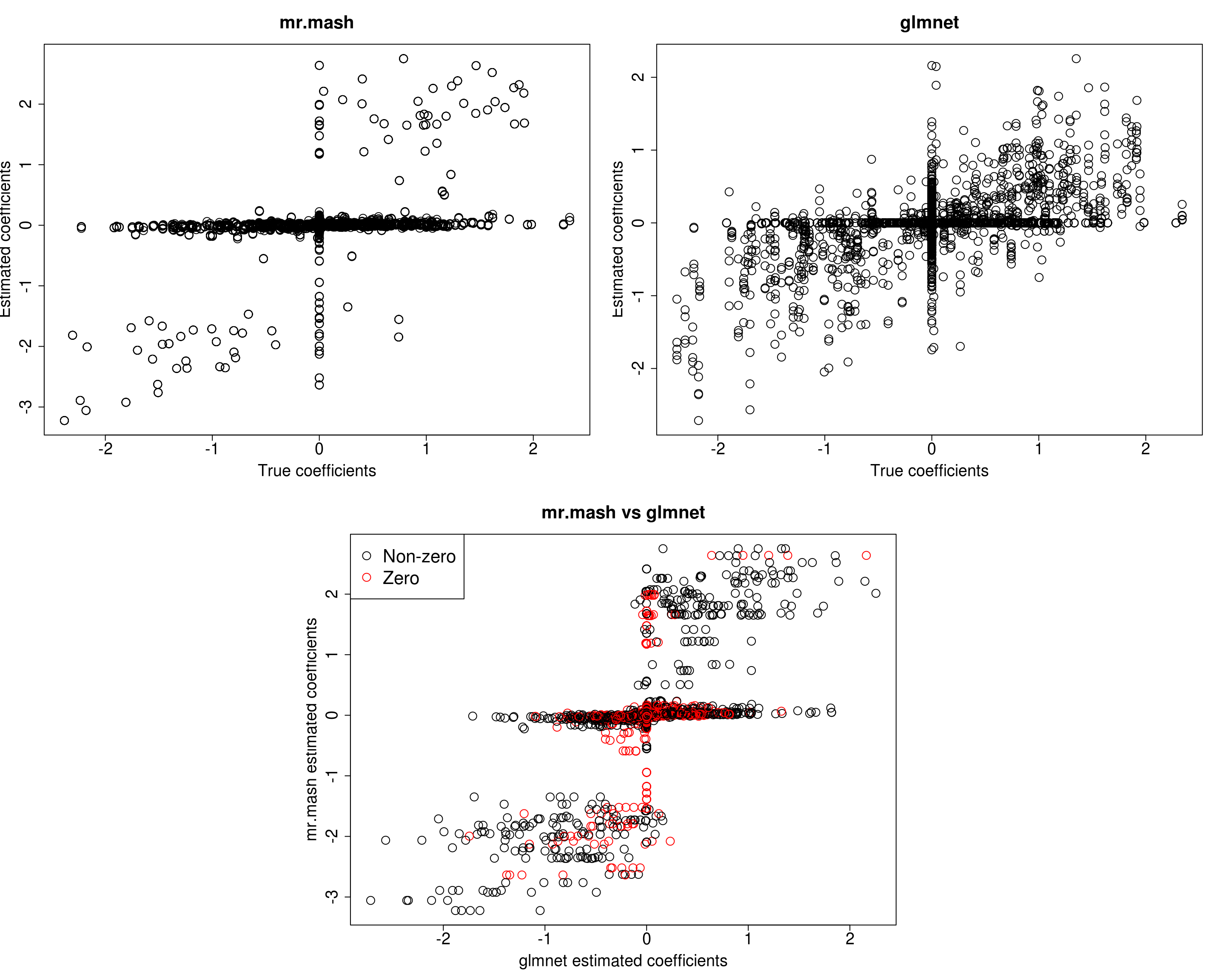
print("Prediction performance with glmnet")[1] "Prediction performance with glmnet"compute_accuracy(Ytest, Yhat_test_glmnet)$bias
[1] 0.7973441 0.7171240 1.1201318 0.9992656 0.9375002
$r2
[1] 0.12560024 0.10044653 0.14357016 0.13204939 0.09516285
$mse
[1] 446.4747 472.2412 509.8068 511.4644 642.4144print("Prediction performance with mr.mash")[1] "Prediction performance with mr.mash"compute_accuracy(Ytest, Yhat_test_mrmash_fixV)$bias
[1] 0.3667682 0.4788130 0.5380369 0.5509452 0.4881568
$r2
[1] 0.06928235 0.11834339 0.12732200 0.13692969 0.08741368
$mse
[1] 576.2796 535.1912 571.8264 567.9749 716.4623Prediction performance looks worse in terms of MSE and \(r^2\) while bias, although still off, is closer to 1. However, looking at the plots of the coefficients, we can see that many coefficients are no longer overshrunk.
For comparison let’s try to repeat the analysis above (updating V) on a sparser scenario, i.e., p_causal=50.
###Set parameters
n <- 600
p <- 1000
p_causal <- 50
r <- 5
r_causal <- r
pve <- 0.5
B_cor <- 1
X_cor <- 0
V_cor <- 0

###Simulate V, B, X and Y
out50 <- mr.mash.alpha:::simulate_mr_mash_data(n, p, p_causal, r, r_causal=r, intercepts = rep(1, r),
                                             pve=pve, B_cor=B_cor, B_scale=0.8, X_cor=X_cor, X_scale=0.8, V_cor=V_cor)

colnames(out50$Y) <- paste0("Y", seq(1, r))
rownames(out50$Y) <- paste0("N", seq(1, n))
colnames(out50$X) <- paste0("X", seq(1, p))
rownames(out50$X) <- paste0("N", seq(1, n))

###Split the data in training and test sets
test_set50 <- sort(sample(x=c(1:n), size=round(n*0.2), replace=FALSE))
Ytrain50 <- out50$Y[-test_set50, ]
Xtrain50 <- out50$X[-test_set50, ]
Ytest50 <- out50$Y[test_set50, ]
Xtest50 <- out50$X[test_set50, ]

###Fit group-lasso
cvfit_glmnet50 <- cv.glmnet(x=Xtrain50, y=Ytrain50, family="mgaussian", alpha=1)
coeff_glmnet50 <- coef(cvfit_glmnet50, s="lambda.min")
Bhat_glmnet50 <- matrix(as.numeric(NA), nrow=p, ncol=r)
ahat_glmnet50 <- vector("numeric", r)
for(i in 1:length(coeff_glmnet50)){
  Bhat_glmnet50[, i] <- as.vector(coeff_glmnet50[[i]])[-1]
  ahat_glmnet50[i] <- as.vector(coeff_glmnet50[[i]])[1]
}
Yhat_test_glmnet50 <- drop(predict(cvfit_glmnet50, newx=Xtest50, s="lambda.min"))

###Fit mr.mash
fit_mrmash50 <- mr.mash(Xtrain50, Ytrain50, S0, tol=1e-2, convergence_criterion="ELBO", update_w0=TRUE,
                     update_w0_method="EM", compute_ELBO=TRUE, standardize=TRUE, verbose=FALSE, update_V=TRUE,
                     mu1_init = Bhat_glmnet50, w0_threshold=1e-8)
Processing the inputs... Done!
Fitting the optimization algorithm... Done!
Processing the outputs... Done!
mr.mash successfully executed in 0.9045867 minutes!Yhat_test_mrmash50 <- predict(fit_mrmash50, Xtest50)Let’s look at the results.
layout(matrix(c(1, 1, 2, 2,
                1, 1, 2, 2,
                0, 3, 3, 0,
                0, 3, 3, 0), 4, 4, byrow = TRUE))

###Plot estimated vs true coeffcients
##mr.mash
plot(out50$B, fit_mrmash50$mu1, main="mr.mash", xlab="True coefficients", ylab="Estimated coefficients",
     cex=2, cex.lab=1.8, cex.main=2, cex.axis=1.8)
##glmnet
plot(out50$B, Bhat_glmnet50, main="glmnet", xlab="True coefficients", ylab="Estimated coefficients",
     cex=2, cex.lab=1.8, cex.main=2, cex.axis=1.8)

###Plot mr.mash vs glmnet estimated coeffcients
colorz <- matrix("black", nrow=p, ncol=r)
zeros <- apply(out50$B, 2, function(x) x==0)
for(i in 1:ncol(colorz)){
  colorz[zeros[, i], i] <- "red"
}

plot(Bhat_glmnet50, fit_mrmash50$mu1, main="mr.mash vs glmnet",
     xlab="glmnet estimated coefficients", ylab="mr.mash estimated coefficients",
     col=colorz, cex=2, cex.lab=1.8, cex.main=2, cex.axis=1.8)
legend("topleft",
       legend = c("Non-zero", "Zero"),
       col = c("black", "red"),
       pch = c(1, 1),
       horiz = FALSE,
cex=2) 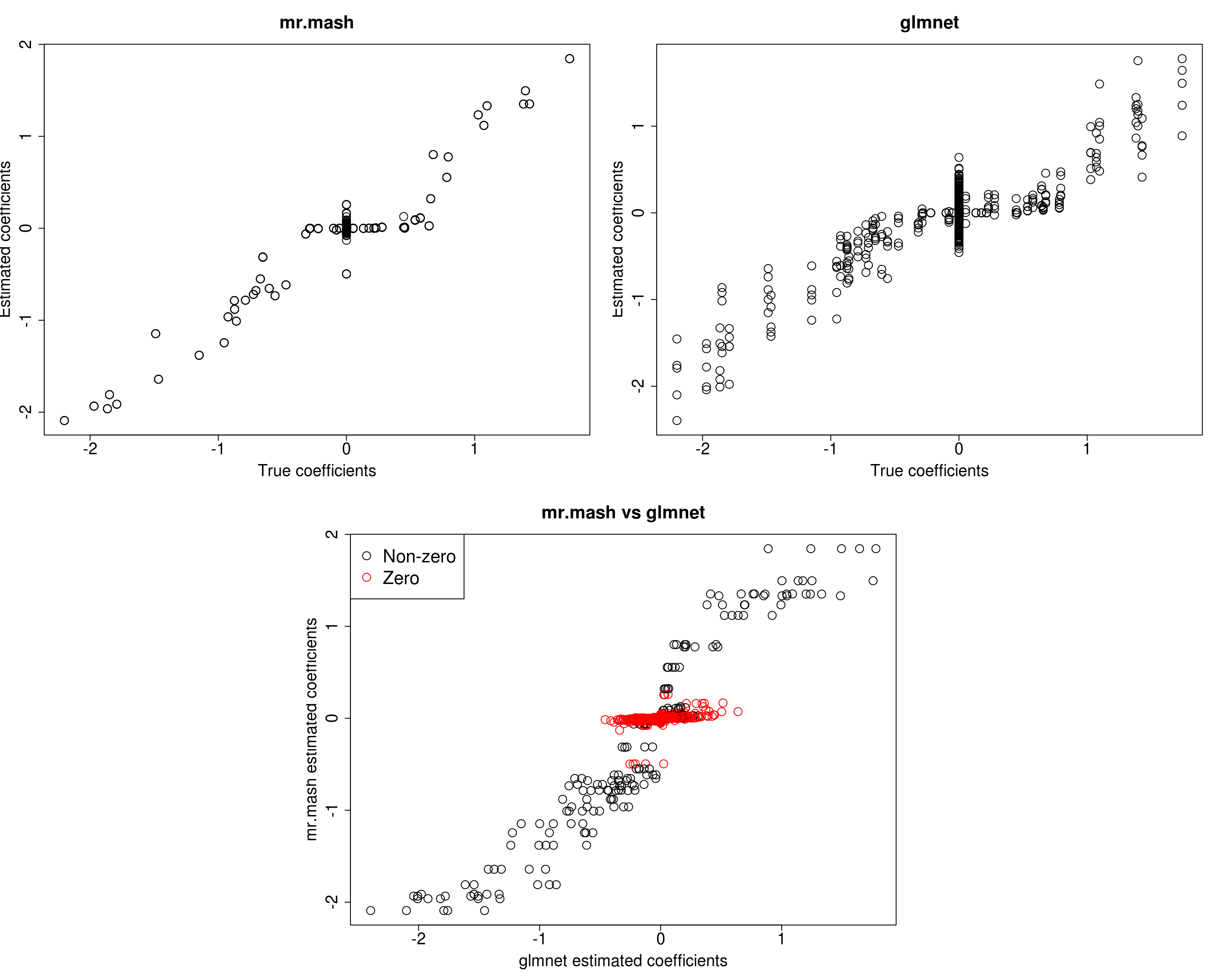
print("Prediction performance with glmnet")[1] "Prediction performance with glmnet"compute_accuracy(Ytest50, Yhat_test_glmnet50)$bias
[1] 1.1055781 1.2342390 0.8929952 1.2093933 1.1997154
$r2
[1] 0.3720343 0.4451268 0.2709590 0.3909355 0.4424055
$mse
[1] 50.11301 49.98023 54.17894 53.96508 46.36995print("Prediction performance with mr.mash")[1] "Prediction performance with mr.mash"compute_accuracy(Ytest50, Yhat_test_mrmash50)$bias
[1] 0.9295387 1.1205934 0.8382439 0.9741666 1.0034935
$r2
[1] 0.4227190 0.5544520 0.3641726 0.4142314 0.4747928
$mse
[1] 46.04314 39.62819 48.00426 51.00798 42.98684print("True V (full data)")[1] "True V (full data)"out50$V [,1] [,2] [,3] [,4] [,5]
[1,] 43.262 0.000 0.000 0.000 0.000
[2,] 0.000 43.262 0.000 0.000 0.000
[3,] 0.000 0.000 43.262 0.000 0.000
[4,] 0.000 0.000 0.000 43.262 0.000
[5,] 0.000 0.000 0.000 0.000 43.262print("Estimated V (training data)")[1] "Estimated V (training data)"fit_mrmash50$V Y1 Y2 Y3 Y4 Y5
Y1 37.0783688 2.693322 2.7229456 3.426152 -0.6935028
Y2 2.6933223 42.243137 2.0293575 1.966294 2.6486737
Y3 2.7229456 2.029357 37.9331012 -2.456907 -0.2269764
Y4 3.4261520 1.966294 -2.4569072 42.752140 -3.0717702
Y5 -0.6935028 2.648674 -0.2269764 -3.071770 43.5576891The results of this simulation look very good in terms of prediction performance, estimation of the coefficients, and estimation of the residual covariance.
Just as an additional test let’s now try to maintain the same signal-to-noise ratio as the first simulation but with fewer total variables, i.e., p=500 and p_causal=250.
###Set parameters
n <- 600
p <- 500
p_causal <- 250
r <- 5
r_causal <- r
pve <- 0.5
B_cor <- 1
X_cor <- 0
V_cor <- 0

###Simulate V, B, X and Y
out500 <- mr.mash.alpha:::simulate_mr_mash_data(n, p, p_causal, r, r_causal=r, intercepts = rep(1, r),
                                             pve=pve, B_cor=B_cor, B_scale=0.8, X_cor=X_cor, X_scale=0.8, V_cor=V_cor)

colnames(out500$Y) <- paste0("Y", seq(1, r))
rownames(out500$Y) <- paste0("N", seq(1, n))
colnames(out500$X) <- paste0("X", seq(1, p))
rownames(out500$X) <- paste0("N", seq(1, n))

###Split the data in training and test sets
test_set500 <- sort(sample(x=c(1:n), size=round(n*0.2), replace=FALSE))
Ytrain500 <- out500$Y[-test_set500, ]
Xtrain500 <- out500$X[-test_set500, ]
Ytest500 <- out500$Y[test_set500, ]
Xtest500 <- out500$X[test_set500, ]

###Fit group-lasso
cvfit_glmnet500 <- cv.glmnet(x=Xtrain500, y=Ytrain500, family="mgaussian", alpha=1)
coeff_glmnet500 <- coef(cvfit_glmnet500, s="lambda.min")
Bhat_glmnet500 <- matrix(as.numeric(NA), nrow=p, ncol=r)
ahat_glmnet500 <- vector("numeric", r)
for(i in 1:length(coeff_glmnet500)){
  Bhat_glmnet500[, i] <- as.vector(coeff_glmnet500[[i]])[-1]
  ahat_glmnet500[i] <- as.vector(coeff_glmnet500[[i]])[1]
}
Yhat_test_glmnet500 <- drop(predict(cvfit_glmnet500, newx=Xtest500, s="lambda.min"))

###Fit mr.mash
fit_mrmash500 <- mr.mash(Xtrain500, Ytrain500, S0, tol=1e-2, convergence_criterion="ELBO", update_w0=TRUE,
                     update_w0_method="EM", compute_ELBO=TRUE, standardize=TRUE, verbose=FALSE, update_V=TRUE,
                     mu1_init = Bhat_glmnet500, w0_threshold=1e-8)
Processing the inputs... Done!
Fitting the optimization algorithm... Done!
Processing the outputs... Done!
mr.mash successfully executed in 1.160227 minutes!Yhat_test_mrmash500 <- predict(fit_mrmash500, Xtest500)Let’s look at the results.
layout(matrix(c(1, 1, 2, 2,
                1, 1, 2, 2,
                0, 3, 3, 0,
                0, 3, 3, 0), 4, 4, byrow = TRUE))

###Plot estimated vs true coeffcients
##mr.mash
plot(out500$B, fit_mrmash500$mu1, main="mr.mash", xlab="True coefficients", ylab="Estimated coefficients",
     cex=2, cex.lab=1.8, cex.main=2, cex.axis=1.8)
##glmnet
plot(out500$B, Bhat_glmnet500, main="glmnet", xlab="True coefficients", ylab="Estimated coefficients",
     cex=2, cex.lab=1.8, cex.main=2, cex.axis=1.8)

###Plot mr.mash vs glmnet estimated coeffcients
colorz <- matrix("black", nrow=p, ncol=r)
zeros <- apply(out500$B, 2, function(x) x==0)
for(i in 1:ncol(colorz)){
  colorz[zeros[, i], i] <- "red"
}

plot(Bhat_glmnet500, fit_mrmash500$mu1, main="mr.mash vs glmnet",
     xlab="glmnet estimated coefficients", ylab="mr.mash estimated coefficients",
     col=colorz, cex=2, cex.lab=1.8, cex.main=2, cex.axis=1.8)
legend("topleft",
       legend = c("Non-zero", "Zero"),
       col = c("black", "red"),
       pch = c(1, 1),
       horiz = FALSE,
cex=2) 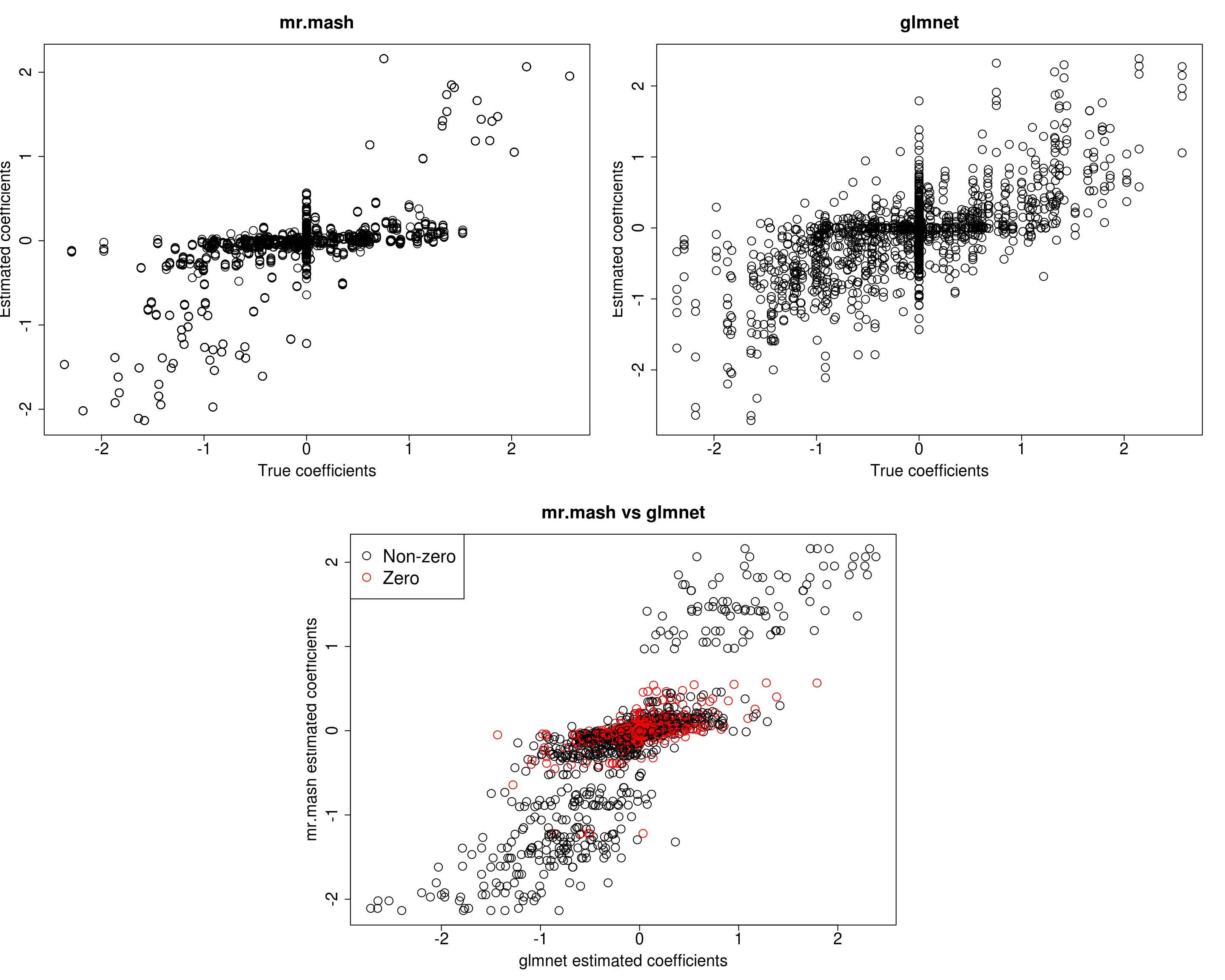
print("Prediction performance with glmnet")[1] "Prediction performance with glmnet"compute_accuracy(Ytest500, Yhat_test_glmnet500)$bias
[1] 0.7460558 0.8379627 0.8827708 1.0150154 0.8988217
$r2
[1] 0.1566151 0.1754140 0.2246133 0.2126951 0.2354353
$mse
[1] 262.5938 307.5913 280.3553 259.2769 265.2623print("Prediction performance with mr.mash")[1] "Prediction performance with mr.mash"compute_accuracy(Ytest500, Yhat_test_mrmash500)$bias
[1] 0.8007963 1.0543346 0.9437460 0.9812104 1.0269983
$r2
[1] 0.1917870 0.2740736 0.2402338 0.2626540 0.2816563
$mse
[1] 249.0113 269.0810 268.4814 242.8198 247.6815print("True V (full data)")[1] "True V (full data)"out500$V [,1] [,2] [,3] [,4] [,5]
[1,] 168.3364 0.0000 0.0000 0.0000 0.0000
[2,] 0.0000 168.3364 0.0000 0.0000 0.0000
[3,] 0.0000 0.0000 168.3364 0.0000 0.0000
[4,] 0.0000 0.0000 0.0000 168.3364 0.0000
[5,] 0.0000 0.0000 0.0000 0.0000 168.3364print("Estimated V (training data)")[1] "Estimated V (training data)"fit_mrmash500$V Y1 Y2 Y3 Y4 Y5
Y1 190.385218 4.826421 31.00999 22.18042 5.743413
Y2 4.826421 181.999035 16.65374 8.40475 9.590063
Y3 31.009989 16.653736 198.77957 39.23005 35.494926
Y4 22.180421 8.404750 39.23005 209.04480 25.167324
Y5 5.743413 9.590063 35.49493 25.16732 194.837000In this last simulation, we can see that mr.mash performs pretty well, even in a denser scenario with fewer variables.
sessionInfo()R version 3.5.1 (2018-07-02)
Platform: x86_64-pc-linux-gnu (64-bit)
Running under: Scientific Linux 7.4 (Nitrogen)
Matrix products: default
BLAS/LAPACK: /software/openblas-0.2.19-el7-x86_64/lib/libopenblas_haswellp-r0.2.19.so
locale:
[1] LC_CTYPE=en_US.UTF-8 LC_NUMERIC=C
[3] LC_TIME=en_US.UTF-8 LC_COLLATE=en_US.UTF-8
[5] LC_MONETARY=en_US.UTF-8 LC_MESSAGES=en_US.UTF-8
[7] LC_PAPER=en_US.UTF-8 LC_NAME=C
[9] LC_ADDRESS=C LC_TELEPHONE=C
[11] LC_MEASUREMENT=en_US.UTF-8 LC_IDENTIFICATION=C
attached base packages:
[1] stats graphics grDevices utils datasets methods base
other attached packages:
[1] glmnet_2.0-16 foreach_1.4.4 Matrix_1.2-15
[4] mr.mash.alpha_0.1-75
loaded via a namespace (and not attached):
[1] MBSP_1.0 Rcpp_1.0.4.6 compiler_3.5.1
[4] later_0.7.5 git2r_0.26.1 workflowr_1.6.1
[7] iterators_1.0.10 tools_3.5.1 digest_0.6.25
[10] evaluate_0.12 lattice_0.20-38 GIGrvg_0.5
[13] yaml_2.2.1 SparseM_1.77 mvtnorm_1.0-12
[16] coda_0.19-3 stringr_1.4.0 knitr_1.20
[19] fs_1.3.1 MatrixModels_0.4-1 rprojroot_1.3-2
[22] grid_3.5.1 glue_1.4.0 R6_2.4.1
[25] rmarkdown_1.10 mixsqp_0.3-43 irlba_2.3.3
[28] magrittr_1.5 whisker_0.3-2 codetools_0.2-15
[31] backports_1.1.5 promises_1.0.1 htmltools_0.3.6
[34] matrixStats_0.55.0 mcmc_0.9-6 MASS_7.3-51.1
[37] httpuv_1.4.5 quantreg_5.36 stringi_1.4.3
[40] MCMCpack_1.4-4