Dense scenario issue - univariate models
Fabio Morgante
June 09, 2020
Last updated: 2020-06-09
Checks: 7 0
Knit directory: mr_mash_test/
This reproducible R Markdown analysis was created with workflowr (version 1.6.2). The Checks tab describes the reproducibility checks that were applied when the results were created. The Past versions tab lists the development history.
Great! Since the R Markdown file has been committed to the Git repository, you know the exact version of the code that produced these results.
Great job! The global environment was empty. Objects defined in the global environment can affect the analysis in your R Markdown file in unknown ways. For reproduciblity it’s best to always run the code in an empty environment.
The command set.seed(20200328) was run prior to running the code in the R Markdown file. Setting a seed ensures that any results that rely on randomness, e.g. subsampling or permutations, are reproducible.
Great job! Recording the operating system, R version, and package versions is critical for reproducibility.
Nice! There were no cached chunks for this analysis, so you can be confident that you successfully produced the results during this run.
Great job! Using relative paths to the files within your workflowr project makes it easier to run your code on other machines.
Great! You are using Git for version control. Tracking code development and connecting the code version to the results is critical for reproducibility.
The results in this page were generated with repository version 2b9d5a8. See the Past versions tab to see a history of the changes made to the R Markdown and HTML files.
Note that you need to be careful to ensure that all relevant files for the analysis have been committed to Git prior to generating the results (you can use wflow_publish or wflow_git_commit). workflowr only checks the R Markdown file, but you know if there are other scripts or data files that it depends on. Below is the status of the Git repository when the results were generated:
Ignored files:
    Ignored:    .sos/
    Ignored:    code/fit_mr_mash.66662433.err
    Ignored:    code/fit_mr_mash.66662433.out
    Ignored:    dsc/.sos/
    Ignored:    dsc/outfiles/
    Ignored:    output/dsc.html
    Ignored:    output/dsc/
    Ignored:    output/dsc_05_18_20.html
    Ignored:    output/dsc_05_18_20/
    Ignored:    output/dsc_05_29_20.html
    Ignored:    output/dsc_05_29_20/
    Ignored:    output/dsc_OLD.html
    Ignored:    output/dsc_OLD/
    Ignored:    output/dsc_test.html
    Ignored:    output/dsc_test/
    Ignored:    output/test_dense_issue.rds
    Ignored:    output/test_sparse_issue.rds

Untracked files:
    Untracked:  code/plot_test.R

Unstaged changes:
    Modified:   dsc/midway2.yml
Note that any generated files, e.g. HTML, png, CSS, etc., are not included in this status report because it is ok for generated content to have uncommitted changes.
These are the previous versions of the repository in which changes were made to the R Markdown (analysis/dense_scenario_issue_univariate.Rmd) and HTML (docs/dense_scenario_issue_univariate.html) files. If you’ve configured a remote Git repository (see ?wflow_git_remote), click on the hyperlinks in the table below to view the files as they were in that past version.
| File | Version | Author | Date | Message |
|---|---|---|---|---|
| Rmd | 2b9d5a8 | fmorgante | 2020-06-09 | Add additional univariate results |
| html | fb32d53 | fmorgante | 2020-06-05 | Build site. |
| Rmd | b3c5072 | fmorgante | 2020-06-05 | Add univariate results |
library(mr.mash.alpha)
library(glmnet)
library(mr.ash.alpha)

###Set options
options(stringsAsFactors = FALSE)

###Set seed
RNGversion("3.5.0")
set.seed(123)
Let’s simulate data with n=600, p=1,000, p_causal=500, r=5, r_causal=5, PVE=0.5, shared effects, independent predictors, and independent residuals. The models will be fitted to the full data.
###Set parameters
n <- 600
p <- 1000
p_causal <- 500
r <- 5
r_causal <- r
pve <- 0.5
B_cor <- 1
X_cor <- 0
V_cor <- 0

###Simulate V, B, X and Y
out <- mr.mash.alpha:::simulate_mr_mash_data(n, p, p_causal, r, r_causal=r, intercepts = rep(1, r),
                                             pve=pve, B_cor=B_cor, B_scale=0.9, X_cor=X_cor, X_scale=0.8, V_cor=V_cor)

colnames(out$Y) <- paste0("Y", seq(1, r))
rownames(out$Y) <- paste0("N", seq(1, n))
colnames(out$X) <- paste0("X", seq(1, p))
rownames(out$X) <- paste0("N", seq(1, n))
We run glmnet with \(\alpha=1\) to obtain an inital estimate for the regression coefficients to provide to mr.ash. Then, we run mr.mash initialized from the mr.ash solution. All the methods are run with standardize=FALSE.
###Compute univariate summary stats needed to compute the prior variances
univ_sumstats <- mr.mash.alpha:::get_univariate_sumstats(out$X, out$Y, standardize=FALSE, standardize.response=FALSE)

###Define matrices to store the coefficients
Bhat_glmnet_univ <- matrix(as.numeric(NA), nrow=p, ncol=r)
Bhat_mrash <- matrix(as.numeric(NA), nrow=p, ncol=r)
Bhat_mrmash_univ <- matrix(as.numeric(NA), nrow=p, ncol=r)

###Loop through responses
for(resp in 1:r){
  ###Fit lasso
  cvfit_glmnet_univ <- cv.glmnet(x=out$X, y=out$Y[, resp], family="gaussian", alpha=1, standardize=FALSE)
  coeff_glmnet_univ <- coef(cvfit_glmnet_univ, s="lambda.min")
  Bhat_glmnet_univ[, resp] <- as.vector(coeff_glmnet_univ)[-1]

  ###Compute prior variances
  grid_univ <- c(0, mr.mash.alpha:::autoselect.mixsd(univ_sumstats$Bhat[, resp], univ_sumstats$Shat[, resp], mult=2))^2

  ###Fit mr.ash
  fit_mrash <- mr.ash.alpha::mr.ash(out$X, out$Y[, resp], sa2=grid_univ, standardize=FALSE, update.pi=TRUE, update.sigma=TRUE,
                                    beta.init=Bhat_glmnet_univ[, resp])
  Bhat_mrash[, resp] <- drop(fit_mrash$beta)

  ###Fit mr.mash
  S0 <- vector("list", length(grid_univ))
  for(i in 1:length(grid_univ)){
    S0[[i]] <- matrix(grid_univ[i], ncol=1, nrow=1)
  }

  fit_mrmash_univ <- mr.mash(out$X, matrix(out$Y[, resp], ncol=1), S0, tol=1e-2, convergence_criterion="ELBO", update_w0=TRUE,
                            update_w0_method="EM", standardize=FALSE, verbose=FALSE, update_V=TRUE, update_V_method="full",
                            w0_threshold=0, mu1_init=fit_mrash$beta)
  Bhat_mrmash_univ[, resp] <- drop(fit_mrmash_univ$mu1)
}
Let’s look at the results for each response.
###Response 1
resp <- 1

layout(matrix(c(1, 1, 2, 2,
                1, 1, 2, 2,
                0, 3, 3, 0,
                0, 3, 3, 0), 4, 4, byrow = TRUE))

###Plot estimated vs true coeffcients
ymax <- max(c(Bhat_mrmash_univ[, resp], Bhat_mrash[, resp]))
ymin <- min(c(Bhat_mrmash_univ[, resp], Bhat_mrash[, resp]))
##mr.mash
plot(out$B[, resp], Bhat_mrmash_univ[, resp], main="mr.mash", xlab="True coefficients", ylab="Estimated coefficients",
     cex=2, cex.lab=1.8, cex.main=2, cex.axis=1.8, ylim=c(ymin, ymax))
##mr.ash
plot(out$B[, resp], Bhat_mrash[, resp], main="mr.ash", xlab="True coefficients", ylab="Estimated coefficients",
     cex=2, cex.lab=1.8, cex.main=2, cex.axis=1.8, ylim=c(ymin, ymax))

###Plot mr.mash vs glmnet estimated coeffcients
colorz <- matrix("black", nrow=p, ncol=1)
zeros <- out$B[, resp]==0
for(i in 1:ncol(colorz)){
  colorz[zeros, i] <- "red"
}

xymax <- max(c(Bhat_mrmash_univ[, resp], Bhat_mrash[, resp]))
xymin <- min(c(Bhat_mrmash_univ[, resp], Bhat_mrash[, resp]))

plot(Bhat_mrash[, resp], Bhat_mrmash_univ[, resp], main="mr.mash vs mr.ash",
     xlab="mr.ash estimated coefficients", ylab="mr.mash estimated coefficients",
     col=colorz, cex=2, cex.lab=1.8, cex.main=2, cex.axis=1.8, xlim=c(xymin, xymax), ylim=c(xymin, xymax))
abline(0, 1)
legend("topleft",
       legend = c("Non-zero", "Zero"),
       col = c("black", "red"),
       pch = c(1, 1),
       horiz = FALSE,
       cex=2)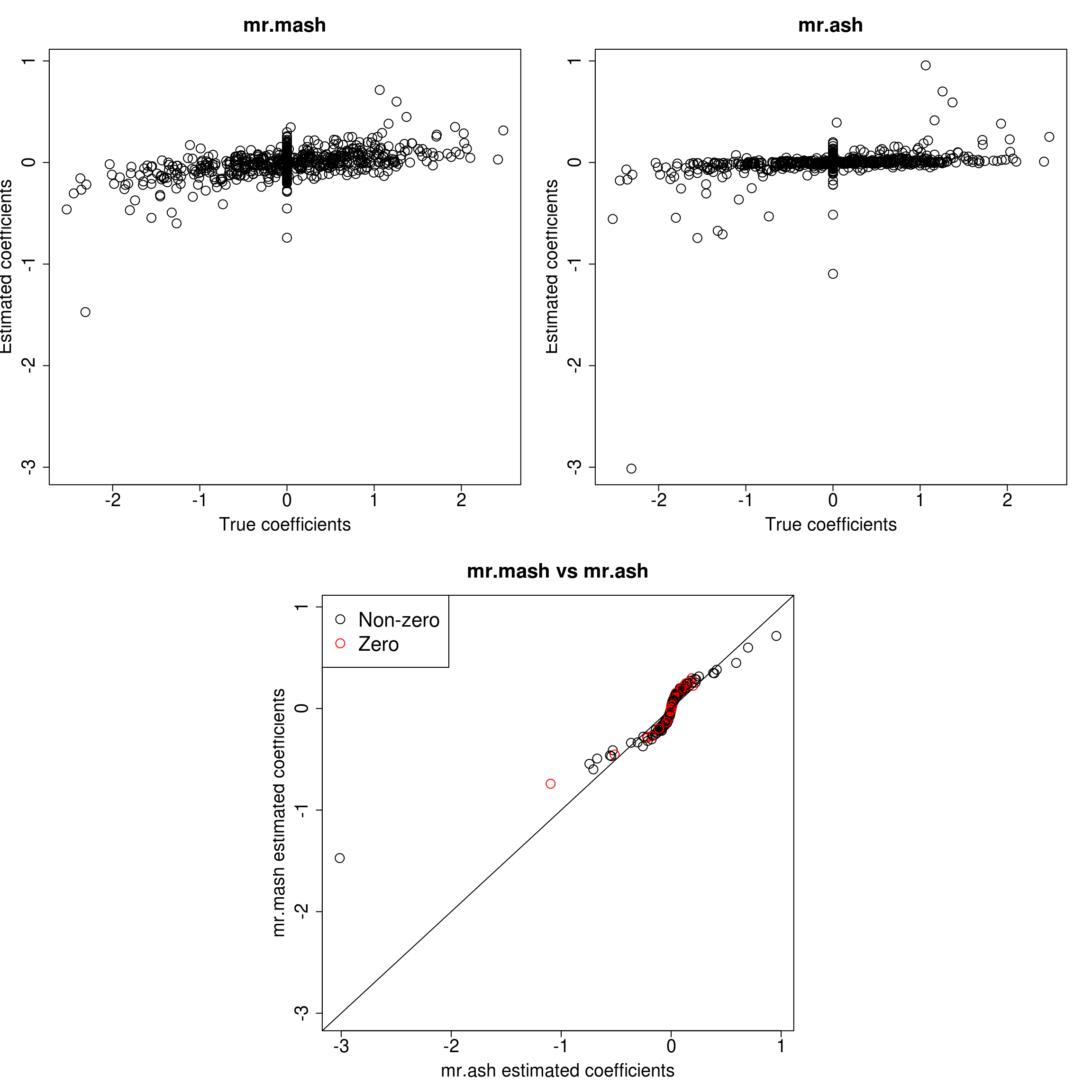
| Version | Author | Date |
|---|---|---|
| fb32d53 | fmorgante | 2020-06-05 |
###Response 2
resp <- 2

layout(matrix(c(1, 1, 2, 2,
                1, 1, 2, 2,
                0, 3, 3, 0,
                0, 3, 3, 0), 4, 4, byrow = TRUE))

###Plot estimated vs true coeffcients
ymax <- max(c(Bhat_mrmash_univ[, resp], Bhat_mrash[, resp]))
ymin <- min(c(Bhat_mrmash_univ[, resp], Bhat_mrash[, resp]))
##mr.mash
plot(out$B[, resp], Bhat_mrmash_univ[, resp], main="mr.mash", xlab="True coefficients", ylab="Estimated coefficients",
     cex=2, cex.lab=1.8, cex.main=2, cex.axis=1.8, ylim=c(ymin, ymax))
##mr.ash
plot(out$B[, resp], Bhat_mrash[, resp], main="mr.ash", xlab="True coefficients", ylab="Estimated coefficients",
     cex=2, cex.lab=1.8, cex.main=2, cex.axis=1.8, ylim=c(ymin, ymax))

###Plot mr.mash vs glmnet estimated coeffcients
colorz <- matrix("black", nrow=p, ncol=1)
zeros <- out$B[, resp]==0
for(i in 1:ncol(colorz)){
  colorz[zeros, i] <- "red"
}

xymax <- max(c(Bhat_mrmash_univ[, resp], Bhat_mrash[, resp]))
xymin <- min(c(Bhat_mrmash_univ[, resp], Bhat_mrash[, resp]))

plot(Bhat_mrash[, resp], Bhat_mrmash_univ[, resp], main="mr.mash vs mr.ash",
     xlab="mr.ash estimated coefficients", ylab="mr.mash estimated coefficients",
     col=colorz, cex=2, cex.lab=1.8, cex.main=2, cex.axis=1.8, xlim=c(xymin, xymax), ylim=c(xymin, xymax))
abline(0, 1)
legend("topleft",
       legend = c("Non-zero", "Zero"),
       col = c("black", "red"),
       pch = c(1, 1),
       horiz = FALSE,
       cex=2)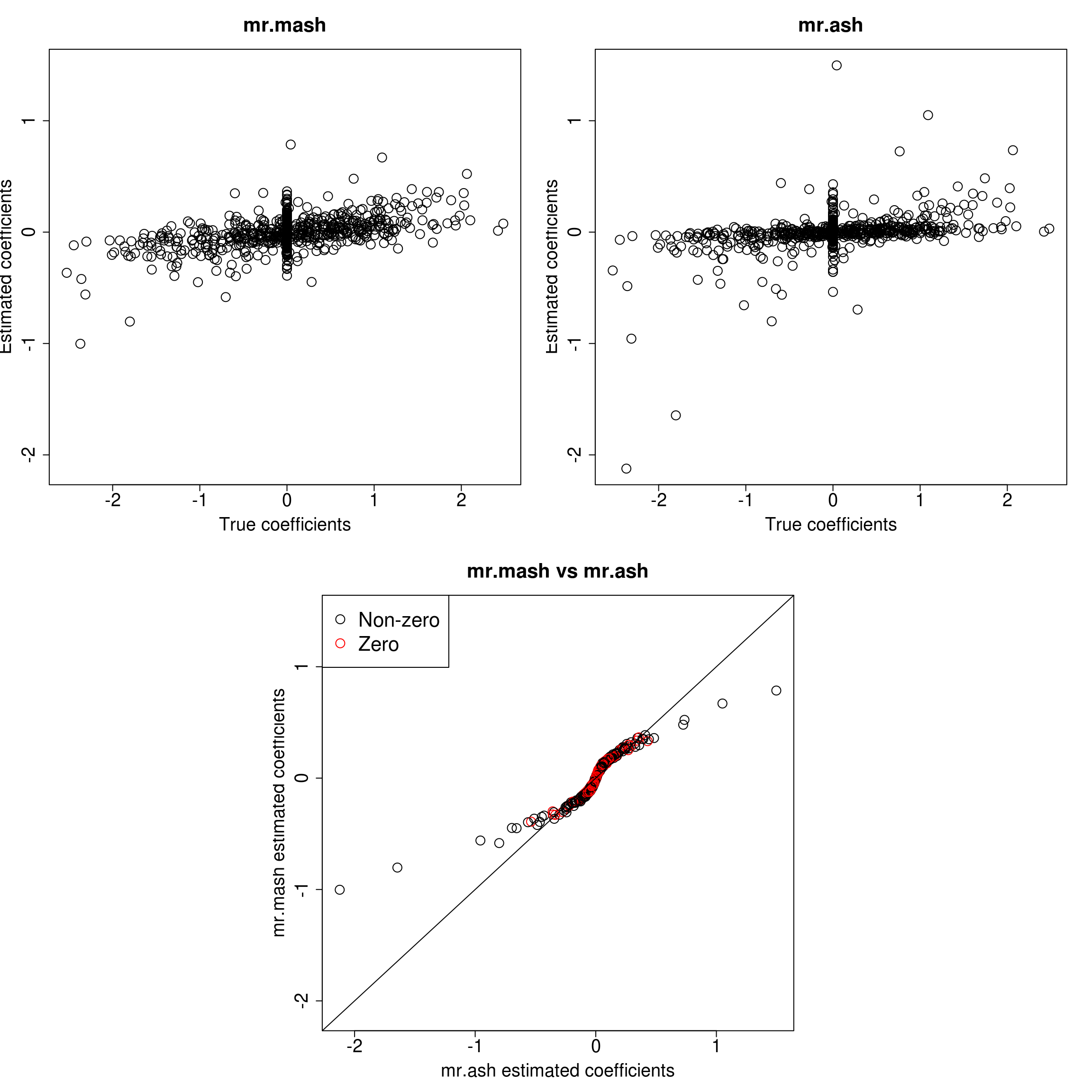
| Version | Author | Date |
|---|---|---|
| fb32d53 | fmorgante | 2020-06-05 |
###Response 3
resp <- 3

layout(matrix(c(1, 1, 2, 2,
                1, 1, 2, 2,
                0, 3, 3, 0,
                0, 3, 3, 0), 4, 4, byrow = TRUE))

###Plot estimated vs true coeffcients
ymax <- max(c(Bhat_mrmash_univ[, resp], Bhat_mrash[, resp]))
ymin <- min(c(Bhat_mrmash_univ[, resp], Bhat_mrash[, resp]))
##mr.mash
plot(out$B[, resp], Bhat_mrmash_univ[, resp], main="mr.mash", xlab="True coefficients", ylab="Estimated coefficients",
     cex=2, cex.lab=1.8, cex.main=2, cex.axis=1.8, ylim=c(ymin, ymax))
##mr.ash
plot(out$B[, resp], Bhat_mrash[, resp], main="mr.ash", xlab="True coefficients", ylab="Estimated coefficients",
     cex=2, cex.lab=1.8, cex.main=2, cex.axis=1.8, ylim=c(ymin, ymax))

###Plot mr.mash vs glmnet estimated coeffcients
colorz <- matrix("black", nrow=p, ncol=1)
zeros <- out$B[, resp]==0
for(i in 1:ncol(colorz)){
  colorz[zeros, i] <- "red"
}

xymax <- max(c(Bhat_mrmash_univ[, resp], Bhat_mrash[, resp]))
xymin <- min(c(Bhat_mrmash_univ[, resp], Bhat_mrash[, resp]))

plot(Bhat_mrash[, resp], Bhat_mrmash_univ[, resp], main="mr.mash vs mr.ash",
     xlab="mr.ash estimated coefficients", ylab="mr.mash estimated coefficients",
     col=colorz, cex=2, cex.lab=1.8, cex.main=2, cex.axis=1.8, xlim=c(xymin, xymax), ylim=c(xymin, xymax))
abline(0, 1)
legend("topleft",
       legend = c("Non-zero", "Zero"),
       col = c("black", "red"),
       pch = c(1, 1),
       horiz = FALSE,
       cex=2)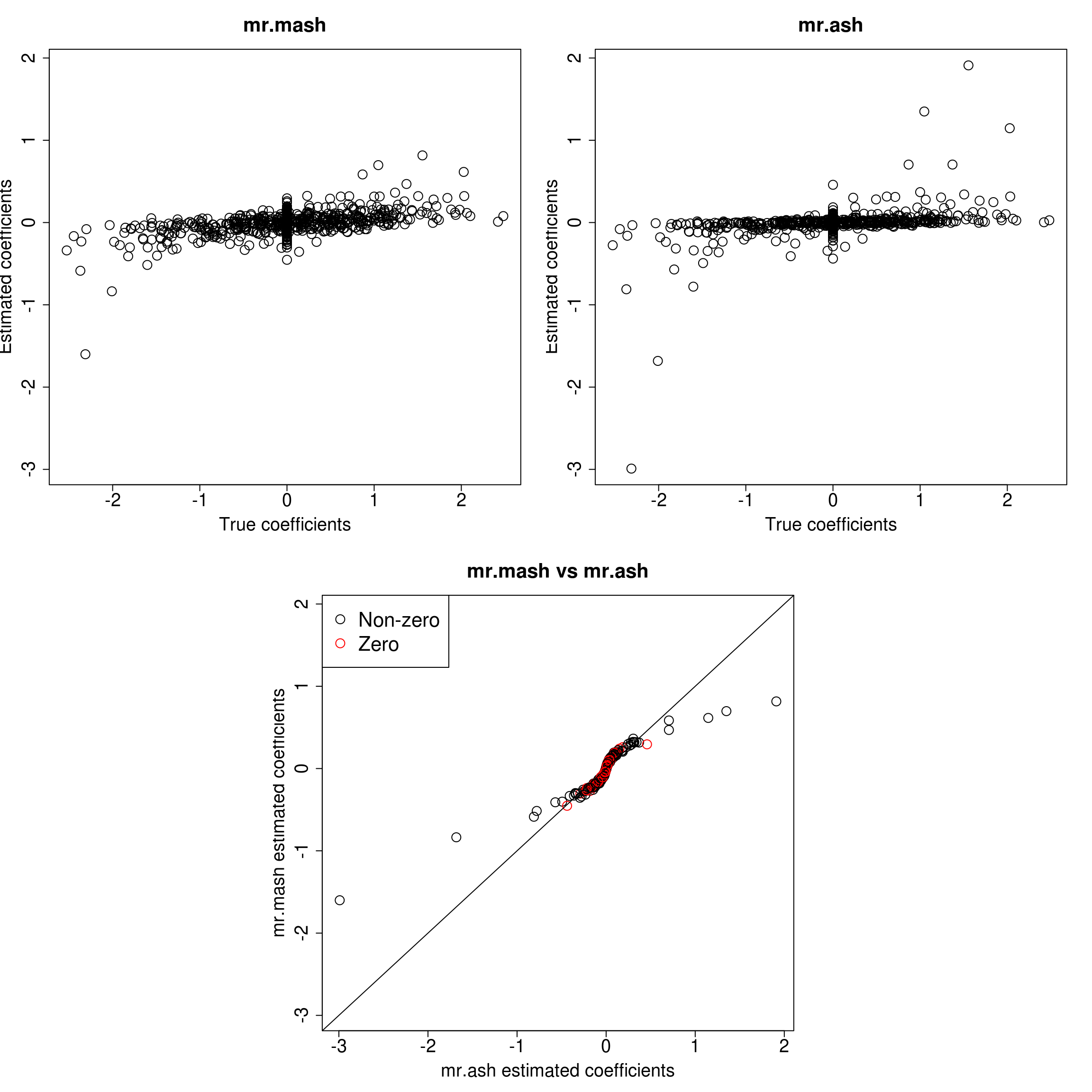
| Version | Author | Date |
|---|---|---|
| fb32d53 | fmorgante | 2020-06-05 |
###Response 4
resp <- 4

layout(matrix(c(1, 1, 2, 2,
                1, 1, 2, 2,
                0, 3, 3, 0,
                0, 3, 3, 0), 4, 4, byrow = TRUE))

###Plot estimated vs true coeffcients
ymax <- max(c(Bhat_mrmash_univ[, resp], Bhat_mrash[, resp]))
ymin <- min(c(Bhat_mrmash_univ[, resp], Bhat_mrash[, resp]))
##mr.mash
plot(out$B[, resp], Bhat_mrmash_univ[, resp], main="mr.mash", xlab="True coefficients", ylab="Estimated coefficients",
     cex=2, cex.lab=1.8, cex.main=2, cex.axis=1.8, ylim=c(ymin, ymax))
##mr.ash
plot(out$B[, resp], Bhat_mrash[, resp], main="mr.ash", xlab="True coefficients", ylab="Estimated coefficients",
     cex=2, cex.lab=1.8, cex.main=2, cex.axis=1.8, ylim=c(ymin, ymax))

###Plot mr.mash vs glmnet estimated coeffcients
colorz <- matrix("black", nrow=p, ncol=1)
zeros <- out$B[, resp]==0
for(i in 1:ncol(colorz)){
  colorz[zeros, i] <- "red"
}

xymax <- max(c(Bhat_mrmash_univ[, resp], Bhat_mrash[, resp]))
xymin <- min(c(Bhat_mrmash_univ[, resp], Bhat_mrash[, resp]))

plot(Bhat_mrash[, resp], Bhat_mrmash_univ[, resp], main="mr.mash vs mr.ash",
     xlab="mr.ash estimated coefficients", ylab="mr.mash estimated coefficients",
     col=colorz, cex=2, cex.lab=1.8, cex.main=2, cex.axis=1.8, xlim=c(xymin, xymax), ylim=c(xymin, xymax))
abline(0, 1)
legend("topleft",
       legend = c("Non-zero", "Zero"),
       col = c("black", "red"),
       pch = c(1, 1),
       horiz = FALSE,
       cex=2)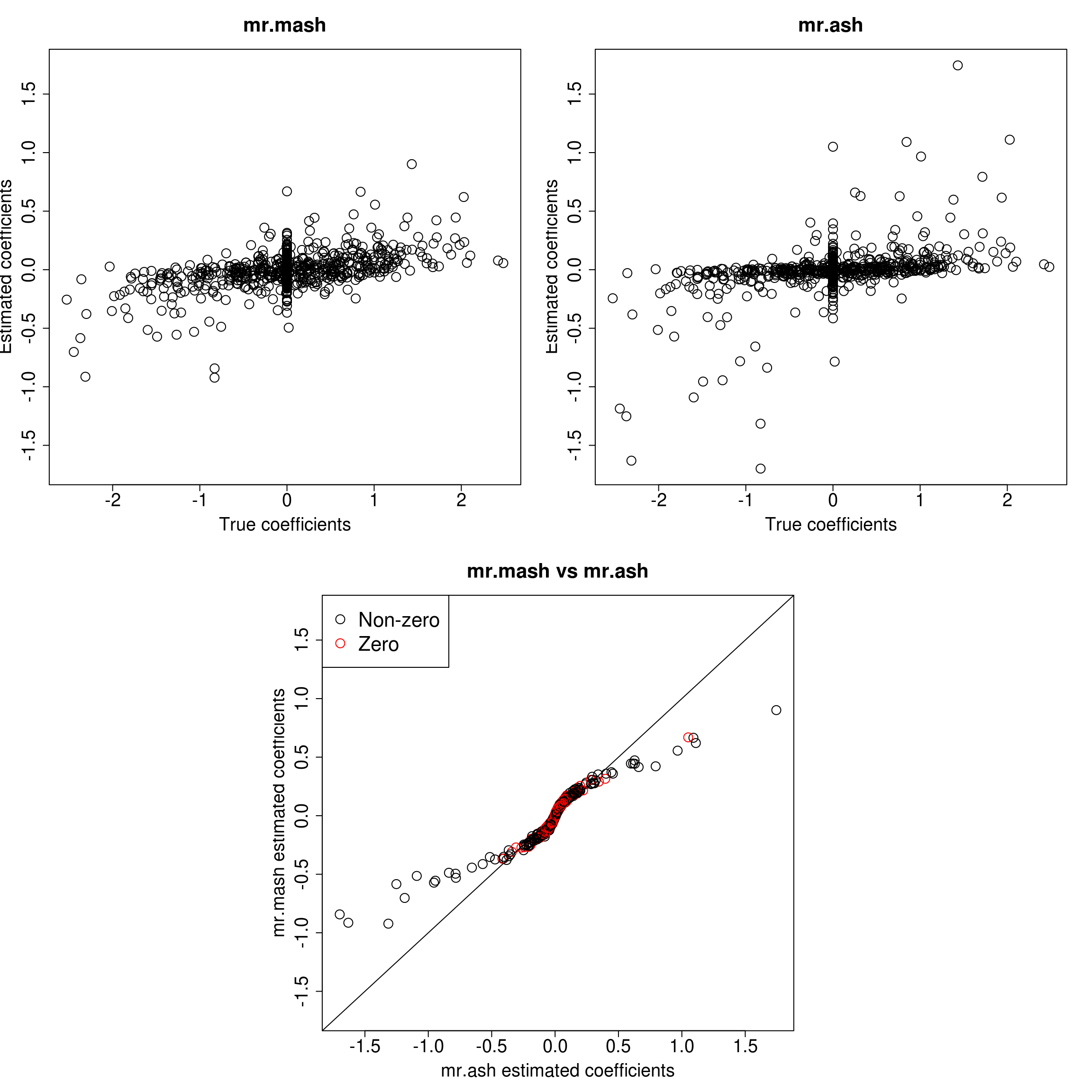
| Version | Author | Date |
|---|---|---|
| fb32d53 | fmorgante | 2020-06-05 |
###Response 5
resp <- 5

layout(matrix(c(1, 1, 2, 2,
                1, 1, 2, 2,
                0, 3, 3, 0,
                0, 3, 3, 0), 4, 4, byrow = TRUE))

###Plot estimated vs true coeffcients
ymax <- max(c(Bhat_mrmash_univ[, resp], Bhat_mrash[, resp]))
ymin <- min(c(Bhat_mrmash_univ[, resp], Bhat_mrash[, resp]))
##mr.mash
plot(out$B[, resp], Bhat_mrmash_univ[, resp], main="mr.mash", xlab="True coefficients", ylab="Estimated coefficients",
     cex=2, cex.lab=1.8, cex.main=2, cex.axis=1.8, ylim=c(ymin, ymax))
##mr.ash
plot(out$B[, resp], Bhat_mrash[, resp], main="mr.ash", xlab="True coefficients", ylab="Estimated coefficients",
     cex=2, cex.lab=1.8, cex.main=2, cex.axis=1.8, ylim=c(ymin, ymax))

###Plot mr.mash vs glmnet estimated coeffcients
colorz <- matrix("black", nrow=p, ncol=1)
zeros <- out$B[, resp]==0
for(i in 1:ncol(colorz)){
  colorz[zeros, i] <- "red"
}

xymax <- max(c(Bhat_mrmash_univ[, resp], Bhat_mrash[, resp]))
xymin <- min(c(Bhat_mrmash_univ[, resp], Bhat_mrash[, resp]))

plot(Bhat_mrash[, resp], Bhat_mrmash_univ[, resp], main="mr.mash vs mr.ash",
     xlab="mr.ash estimated coefficients", ylab="mr.mash estimated coefficients",
     col=colorz, cex=2, cex.lab=1.8, cex.main=2, cex.axis=1.8, xlim=c(xymin, xymax), ylim=c(xymin, xymax))
abline(0, 1)
legend("topleft",
       legend = c("Non-zero", "Zero"),
       col = c("black", "red"),
       pch = c(1, 1),
       horiz = FALSE,
       cex=2)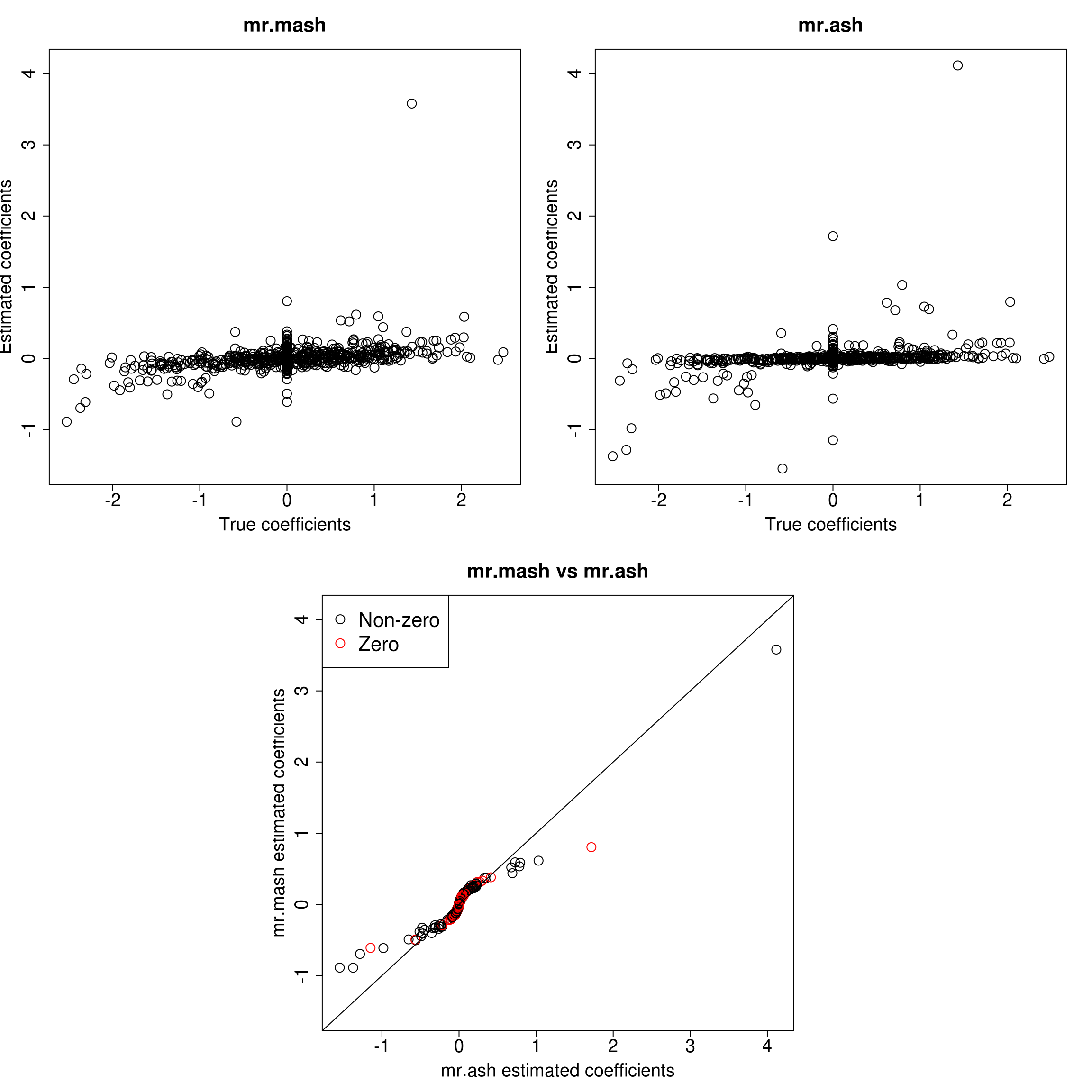
| Version | Author | Date |
|---|---|---|
| fb32d53 | fmorgante | 2020-06-05 |
As we can see, mr.mash shrinks large coeffcients more than mr.ash. Now, we need to understand why these two implementations are giving different results. We will start by making sure that the two methods give the same results with fixed residual variance (and properly scaled prior variances in the case of mr.ash).
###Define matrices to store the coefficients
Bhat_mrash_fixV <- matrix(as.numeric(NA), nrow=p, ncol=r)
Bhat_mrmash_univ_fixV <- matrix(as.numeric(NA), nrow=p, ncol=r)

###Loop through responses
for(resp in 1:r){
  ###Compute prior variances
  grid_univ <- c(0, mr.mash.alpha:::autoselect.mixsd(univ_sumstats$Bhat[, resp], univ_sumstats$Shat[, resp], mult=2))^2

  ###Fit mr.ash
  fit_mrash_fixV <-mr.ash(out$X, out$Y[, resp], standardize=FALSE, update.pi=TRUE, update.sigma=FALSE, sa2 = grid_univ/var(out$Y[,resp]),
                          beta.init=Bhat_glmnet_univ[, resp], sigma2 = var(out$Y[,resp]), pi = rep(1/length(grid_univ), length(grid_univ)))
  Bhat_mrash_fixV[, resp] <- drop(fit_mrash_fixV$beta)

  ###Fit mr.mash
  S0 <- vector("list", length(grid_univ))
  for(i in 1:length(grid_univ)){
    S0[[i]] <- matrix(grid_univ[i], ncol=1, nrow=1)
  }

  fit_mrmash_univ_fixV <- mr.mash(out$X, matrix(out$Y[, resp], ncol=1), S0, tol=1e-4, convergence_criterion="ELBO", update_w0=TRUE,
                            update_w0_method="EM", standardize=FALSE, verbose=FALSE, update_V=FALSE, update_V_method="full",
                            w0_threshold=0, mu1_init=fit_mrash_fixV$beta, V=matrix(var(out$Y[,resp]), 1, 1), e=0)
  Bhat_mrmash_univ_fixV[, resp] <- drop(fit_mrmash_univ_fixV$mu1)
}
Let’s look at the results for each response.
layout(matrix(c(1, 1, 2, 2, 3, 3,
                1, 1, 2, 2, 3, 3,
                0, 4, 4, 5, 5, 0,
                0, 4, 4, 5, 5, 0), 4, 6, byrow = TRUE))

resp <- 1

xymax <- max(c(Bhat_mrmash_univ_fixV[, resp], Bhat_mrash_fixV[, resp]))
xymin <- min(c(Bhat_mrmash_univ_fixV[, resp], Bhat_mrash_fixV[, resp]))

plot(Bhat_mrash_fixV[, resp], Bhat_mrmash_univ_fixV[, resp], main="mr.mash vs mr.ash",
     xlab="mr.ash estimated coefficients", ylab="mr.mash estimated coefficients",
     cex=2, cex.lab=1.8, cex.main=2, cex.axis=1.8, xlim=c(xymin, xymax), ylim=c(xymin, xymax))
abline(0, 1)

resp <- 2

xymax <- max(c(Bhat_mrmash_univ_fixV[, resp], Bhat_mrash_fixV[, resp]))
xymin <- min(c(Bhat_mrmash_univ_fixV[, resp], Bhat_mrash_fixV[, resp]))

plot(Bhat_mrash_fixV[, resp], Bhat_mrmash_univ_fixV[, resp], main="mr.mash vs mr.ash",
     xlab="mr.ash estimated coefficients", ylab="mr.mash estimated coefficients",
     cex=2, cex.lab=1.8, cex.main=2, cex.axis=1.8, xlim=c(xymin, xymax), ylim=c(xymin, xymax))
abline(0, 1)

resp <- 3

xymax <- max(c(Bhat_mrmash_univ_fixV[, resp], Bhat_mrash_fixV[, resp]))
xymin <- min(c(Bhat_mrmash_univ_fixV[, resp], Bhat_mrash_fixV[, resp]))

plot(Bhat_mrash_fixV[, resp], Bhat_mrmash_univ_fixV[, resp], main="mr.mash vs mr.ash",
     xlab="mr.ash estimated coefficients", ylab="mr.mash estimated coefficients",
     cex=2, cex.lab=1.8, cex.main=2, cex.axis=1.8, xlim=c(xymin, xymax), ylim=c(xymin, xymax))
abline(0, 1)

resp <- 4

xymax <- max(c(Bhat_mrmash_univ_fixV[, resp], Bhat_mrash_fixV[, resp]))
xymin <- min(c(Bhat_mrmash_univ_fixV[, resp], Bhat_mrash_fixV[, resp]))

plot(Bhat_mrash_fixV[, resp], Bhat_mrmash_univ_fixV[, resp], main="mr.mash vs mr.ash",
     xlab="mr.ash estimated coefficients", ylab="mr.mash estimated coefficients",
     cex=2, cex.lab=1.8, cex.main=2, cex.axis=1.8, xlim=c(xymin, xymax), ylim=c(xymin, xymax))
abline(0, 1)

resp <- 5

xymax <- max(c(Bhat_mrmash_univ_fixV[, resp], Bhat_mrash_fixV[, resp]))
xymin <- min(c(Bhat_mrmash_univ_fixV[, resp], Bhat_mrash_fixV[, resp]))

plot(Bhat_mrash_fixV[, resp], Bhat_mrmash_univ_fixV[, resp], main="mr.mash vs mr.ash",
     xlab="mr.ash estimated coefficients", ylab="mr.mash estimated coefficients",
     cex=2, cex.lab=1.8, cex.main=2, cex.axis=1.8, xlim=c(xymin, xymax), ylim=c(xymin, xymax))
abline(0, 1)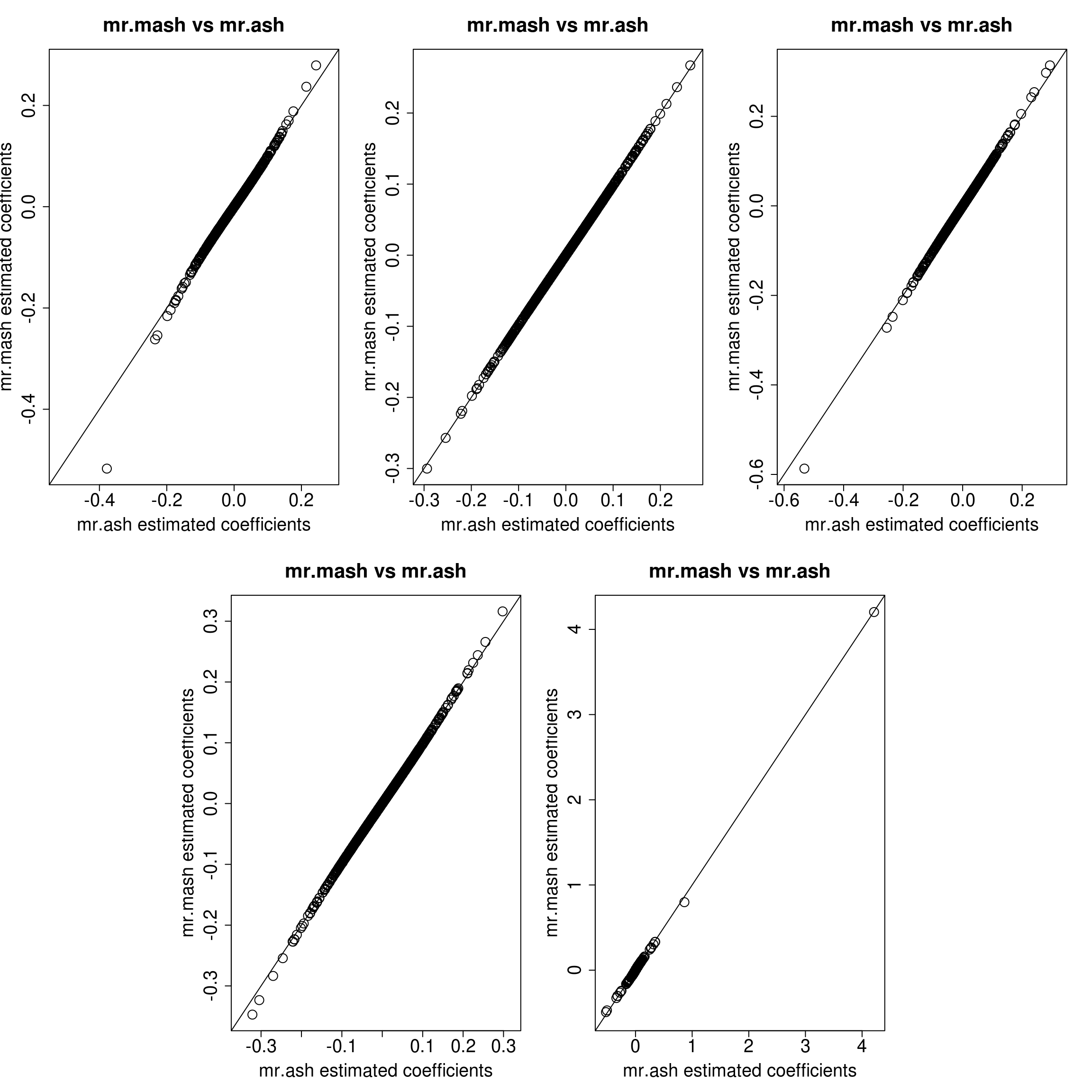
| Version | Author | Date |
|---|---|---|
| fb32d53 | fmorgante | 2020-06-05 |
The results look very similar, so the coordinate ascent algorithm and the update of the mixture weights should not be the culprit of the differences seen in the first plots. N.B. we still had to make the convergence criterion stricter in mr.mash to reach this level of agreement.
After a conversation, Matthew and I discovered that I have been providing a grid that was not sensible to mr.ash. This is because of the different (scaled) parameterization of the prior, \(b \sim N(0, \sigma^2 \sigma^2_b)\). This might account for all the differences between mr.ash and mr.mash we have seen. To test this hypothesis, we will use this strategy: 1. Fit mr.ash with a sufficiently dense and wide grid. 2. Fit mr.mash with the same grid multiplied by the estimated residual variance from mr.ash In this way, the two grids will be approximately equivalent, given the two different parameterizations of the model.
###Compute grid of prior variances for mr.ash
grid_mrash <- c(0, sort(10^seq(2,-3.5,length.out = 500)))

###Define matrices to store the coefficients
Bhat_mrash_eqgrid <- matrix(as.numeric(NA), nrow=p, ncol=r)
Bhat_mrmash_univ_eqgrid <- matrix(as.numeric(NA), nrow=p, ncol=r)

###Loop through responses
for(resp in 1:r){

  ###Fit mr.ash
  fit_mrash_eqgrid <- mr.ash.alpha::mr.ash(out$X, out$Y[, resp], sa2=grid_mrash, standardize=FALSE, update.pi=TRUE, update.sigma=TRUE,
                                    beta.init=Bhat_glmnet_univ[, resp])
  Bhat_mrash_eqgrid[, resp] <- drop(fit_mrash_eqgrid$beta)

  ###Fit mr.mash
  S0 <- list()
  for(i in 1:length(grid_mrash)){
    S0[[i]] <- matrix(grid_mrash[i]*fit_mrash_eqgrid$sigma2, ncol=1, nrow=1)
  }

  fit_mrmash_univ_eqgrid <- mr.mash(out$X, matrix(out$Y[, resp], ncol=1), S0, tol=1e-4, convergence_criterion="ELBO", update_w0=TRUE,
                                    update_w0_method="EM", standardize=FALSE, verbose=FALSE, update_V=TRUE, update_V_method="full",
                                    w0_threshold=0, mu1_init=matrix(Bhat_glmnet_univ[, resp], ncol=1), e=0)
  Bhat_mrmash_univ_eqgrid[, resp] <- drop(fit_mrmash_univ_eqgrid$mu1)
}
layout(matrix(c(1, 1, 2, 2, 3, 3,
1, 1, 2, 2, 3, 3,
0, 4, 4, 5, 5, 0,
0, 4, 4, 5, 5, 0), 4, 6, byrow = TRUE))
resp <- 1
xymax <- max(c(Bhat_mrmash_univ_eqgrid[, resp], Bhat_mrash_eqgrid[, resp]))
xymin <- min(c(Bhat_mrmash_univ_eqgrid[, resp], Bhat_mrash_eqgrid[, resp]))
plot(Bhat_mrash_eqgrid[, resp], Bhat_mrmash_univ_eqgrid[, resp], main="mr.mash vs mr.ash",
xlab="mr.ash estimated coefficients", ylab="mr.mash estimated coefficients",
cex=2, cex.lab=1.8, cex.main=2, cex.axis=1.8, xlim=c(xymin, xymax), ylim=c(xymin, xymax))
abline(0, 1)
resp <- 2
xymax <- max(c(Bhat_mrmash_univ_eqgrid[, resp], Bhat_mrash_eqgrid[, resp]))
xymin <- min(c(Bhat_mrmash_univ_eqgrid[, resp], Bhat_mrash_eqgrid[, resp]))
plot(Bhat_mrash_eqgrid[, resp], Bhat_mrmash_univ_eqgrid[, resp], main="mr.mash vs mr.ash",
xlab="mr.ash estimated coefficients", ylab="mr.mash estimated coefficients",
cex=2, cex.lab=1.8, cex.main=2, cex.axis=1.8, xlim=c(xymin, xymax), ylim=c(xymin, xymax))
abline(0, 1)
resp <- 3
xymax <- max(c(Bhat_mrmash_univ_eqgrid[, resp], Bhat_mrash_eqgrid[, resp]))
xymin <- min(c(Bhat_mrmash_univ_eqgrid[, resp], Bhat_mrash_eqgrid[, resp]))
plot(Bhat_mrash_eqgrid[, resp], Bhat_mrmash_univ_eqgrid[, resp], main="mr.mash vs mr.ash",
xlab="mr.ash estimated coefficients", ylab="mr.mash estimated coefficients",
cex=2, cex.lab=1.8, cex.main=2, cex.axis=1.8, xlim=c(xymin, xymax), ylim=c(xymin, xymax))
abline(0, 1)
resp <- 4
xymax <- max(c(Bhat_mrmash_univ_eqgrid[, resp], Bhat_mrash_eqgrid[, resp]))
xymin <- min(c(Bhat_mrmash_univ_eqgrid[, resp], Bhat_mrash_eqgrid[, resp]))
plot(Bhat_mrash_eqgrid[, resp], Bhat_mrmash_univ_eqgrid[, resp], main="mr.mash vs mr.ash",
xlab="mr.ash estimated coefficients", ylab="mr.mash estimated coefficients",
cex=2, cex.lab=1.8, cex.main=2, cex.axis=1.8, xlim=c(xymin, xymax), ylim=c(xymin, xymax))
abline(0, 1)
resp <- 5
xymax <- max(c(Bhat_mrmash_univ_eqgrid[, resp], Bhat_mrash_eqgrid[, resp]))
xymin <- min(c(Bhat_mrmash_univ_eqgrid[, resp], Bhat_mrash_eqgrid[, resp]))
plot(Bhat_mrash_eqgrid[, resp], Bhat_mrmash_univ_eqgrid[, resp], main="mr.mash vs mr.ash",
xlab="mr.ash estimated coefficients", ylab="mr.mash estimated coefficients",
cex=2, cex.lab=1.8, cex.main=2, cex.axis=1.8, xlim=c(xymin, xymax), ylim=c(xymin, xymax))
abline(0, 1)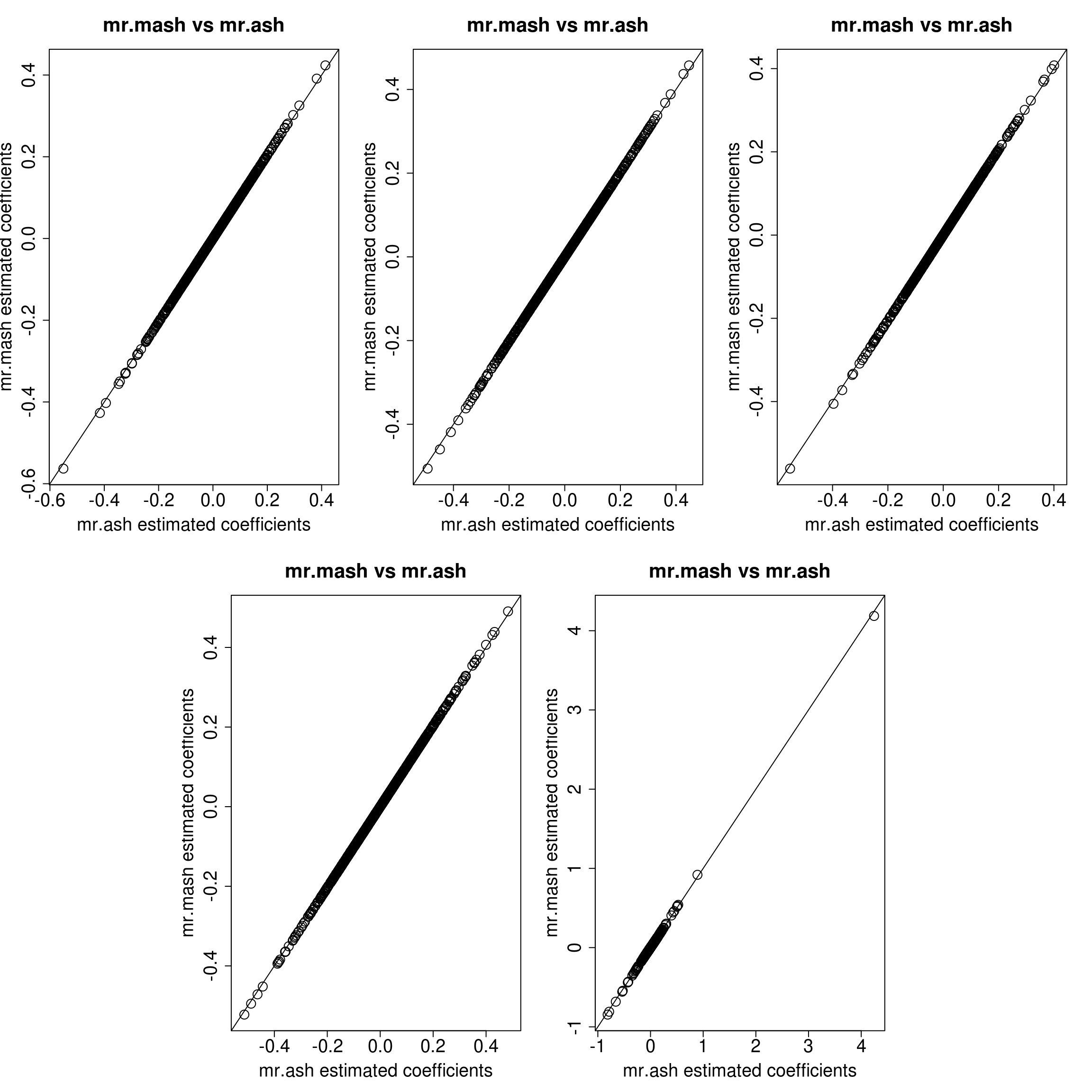
The results are now essentially the same! The remaining differences (I believe) can be attributed to the slightly different solutions achieved due to the different convergence checks used in the two software (i.e., ELBO in mr.mash and mixture weights in mr.ash).
So, the take-home messages are: 1. At least in this example, the two different parameterizations lead essentially to the same results. 2. One needs to be careful in choosing the grid of prior variances, especially with the scaled parameterization, which is less intuitive!
sessionInfo()R version 3.5.1 (2018-07-02)
Platform: x86_64-pc-linux-gnu (64-bit)
Running under: Scientific Linux 7.4 (Nitrogen)
Matrix products: default
BLAS/LAPACK: /software/openblas-0.2.19-el7-x86_64/lib/libopenblas_haswellp-r0.2.19.so
locale:
[1] LC_CTYPE=en_US.UTF-8 LC_NUMERIC=C
[3] LC_TIME=en_US.UTF-8 LC_COLLATE=en_US.UTF-8
[5] LC_MONETARY=en_US.UTF-8 LC_MESSAGES=en_US.UTF-8
[7] LC_PAPER=en_US.UTF-8 LC_NAME=C
[9] LC_ADDRESS=C LC_TELEPHONE=C
[11] LC_MEASUREMENT=en_US.UTF-8 LC_IDENTIFICATION=C
attached base packages:
[1] stats graphics grDevices utils datasets methods base
other attached packages:
[1] mr.ash.alpha_0.1-32 glmnet_2.0-16 foreach_1.4.4
[4] Matrix_1.2-15 mr.mash.alpha_0.1-79
loaded via a namespace (and not attached):
[1] MBSP_1.0 Rcpp_1.0.4.6 compiler_3.5.1
[4] later_0.7.5 git2r_0.26.1 workflowr_1.6.2
[7] iterators_1.0.10 tools_3.5.1 digest_0.6.25
[10] evaluate_0.12 lattice_0.20-38 GIGrvg_0.5
[13] yaml_2.2.1 SparseM_1.77 mvtnorm_1.1-0
[16] coda_0.19-3 stringr_1.4.0 knitr_1.20
[19] fs_1.3.1 MatrixModels_0.4-1 rprojroot_1.3-2
[22] grid_3.5.1 glue_1.4.0 R6_2.4.1
[25] rmarkdown_1.10 mixsqp_0.3-43 irlba_2.3.3
[28] magrittr_1.5 whisker_0.3-2 codetools_0.2-15
[31] backports_1.1.5 promises_1.0.1 htmltools_0.3.6
[34] matrixStats_0.56.0 mcmc_0.9-6 MASS_7.3-51.1
[37] httpuv_1.4.5 quantreg_5.36 stringi_1.4.3
[40] MCMCpack_1.4-4