Two active responses case
Fabio Morgante
May 28, 2020
Last updated: 2020-05-28
Checks: 7 0
Knit directory: mr_mash_test/
This reproducible R Markdown analysis was created with workflowr (version 1.6.1). The Checks tab describes the reproducibility checks that were applied when the results were created. The Past versions tab lists the development history.
Great! Since the R Markdown file has been committed to the Git repository, you know the exact version of the code that produced these results.
Great job! The global environment was empty. Objects defined in the global environment can affect the analysis in your R Markdown file in unknown ways. For reproduciblity it’s best to always run the code in an empty environment.
The command set.seed(20200328) was run prior to running the code in the R Markdown file. Setting a seed ensures that any results that rely on randomness, e.g. subsampling or permutations, are reproducible.
Great job! Recording the operating system, R version, and package versions is critical for reproducibility.
Nice! There were no cached chunks for this analysis, so you can be confident that you successfully produced the results during this run.
Great job! Using relative paths to the files within your workflowr project makes it easier to run your code on other machines.
Great! You are using Git for version control. Tracking code development and connecting the code version to the results is critical for reproducibility.
The results in this page were generated with repository version 8fde94a. See the Past versions tab to see a history of the changes made to the R Markdown and HTML files.
Note that you need to be careful to ensure that all relevant files for the analysis have been committed to Git prior to generating the results (you can use wflow_publish or wflow_git_commit). workflowr only checks the R Markdown file, but you know if there are other scripts or data files that it depends on. Below is the status of the Git repository when the results were generated:
Ignored files:
    Ignored:    .sos/
    Ignored:    code/fit_mr_mash.66662433.err
    Ignored:    code/fit_mr_mash.66662433.out
    Ignored:    dsc/.sos/
    Ignored:    dsc/outfiles/
    Ignored:    output/dsc.html
    Ignored:    output/dsc/
    Ignored:    output/dsc_05_18_20.html
    Ignored:    output/dsc_05_18_20/
    Ignored:    output/dsc_05_24_20.html
    Ignored:    output/dsc_05_24_20/
    Ignored:    output/dsc_OLD.html
    Ignored:    output/dsc_OLD/
    Ignored:    output/dsc_test.html
    Ignored:    output/dsc_test/

Untracked files:
    Untracked:  Rplots.pdf
    Untracked:  code/plot_test.R

Unstaged changes:
    Modified:   dsc/midway2.yml
Note that any generated files, e.g. HTML, png, CSS, etc., are not included in this status report because it is ok for generated content to have uncommitted changes.
These are the previous versions of the repository in which changes were made to the R Markdown (analysis/two_active_responses_issue.Rmd) and HTML (docs/two_active_responses_issue.html) files. If you’ve configured a remote Git repository (see ?wflow_git_remote), click on the hyperlinks in the table below to view the files as they were in that past version.
| File | Version | Author | Date | Message |
|---|---|---|---|---|
| Rmd | 8fde94a | fmorgante | 2020-05-28 | Add more investigations |
| html | 2682eba | fmorgante | 2020-05-28 | Build site. |
| Rmd | 738798c | fmorgante | 2020-05-28 | Add more investigations |
| html | 5e13912 | fmorgante | 2020-05-27 | Build site. |
| Rmd | 068beb2 | fmorgante | 2020-05-27 | Increase cex |
| html | f2b6bf8 | fmorgante | 2020-05-27 | Build site. |
| Rmd | a626e53 | fmorgante | 2020-05-27 | Increase cex |
| html | 7dad46c | fmorgante | 2020-05-27 | Build site. |
| Rmd | 465b10d | fmorgante | 2020-05-27 | Add case study with only two causal tissues out of five |
library(mr.mash.alpha)
library(glmnet)
Loading required package: MatrixLoading required package: foreachLoaded glmnet 2.0-16###Set options
options(stringsAsFactors = FALSE)Let’s simulate data with n=600, p=1,000, p_causal=50, r=5, r_causal=2, PVE=0.5, shared effects, independent predictors, and lowly correlated residuals. The models will be fitted to the training data (80% of the full data).
###Set seed
set.seed(123)

###Set parameters
n <- 600
p <- 1000
p_causal <- 50
r <- 5
r_causal <- 2

###Simulate V, B, X and Y
out <- mr.mash.alpha:::simulate_mr_mash_data(n, p, p_causal, r, r_causal, intercepts = rep(1, r),
                                             pve=0.5, B_cor=1, B_scale=0.8, X_cor=0, X_scale=0.8, V_cor=0.15)

colnames(out$Y) <- paste0("Y", seq(1, r))
rownames(out$Y) <- paste0("N", seq(1, n))
colnames(out$X) <- paste0("X", seq(1, p))
rownames(out$X) <- paste0("N", seq(1, n))

###Split the data in training and test sets
test_set <- sort(sample(x=c(1:n), size=round(n*0.2), replace=FALSE))
Ytrain <- out$Y[-test_set, ]
Xtrain <- out$X[-test_set, ]
Ytest <- out$Y[test_set, ]
Xtest <- out$X[test_set, ]

head(out$B[out$causal_variables, ])
[,1] [,2] [,3] [,4] [,5]
[1,] 0.07316118 0.07316118 0 0 0
[2,] 0.44056603 0.44056603 0 0 0
[3,] 0.31699557 0.31699557 0 0 0
[4,] -0.95215593 -0.95215593 0 0 0
[5,] 0.07038939 0.07038939 0 0 0
[6,] -0.92892961 -0.92892961 0 0 0We build the mixture prior as usual including zero matrix, identity matrix, rank-1 matrices, low, medium and high heterogeneity matrices, shared matrix, each scaled by a grid from 0.1 to 2.1 in steps of 0.2.
grid <- seq(0.1, 2.1, 0.2)
S0 <- mr.mash.alpha:::compute_cov_canonical(ncol(Ytrain), singletons=TRUE, hetgrid=c(0, 0.25, 0.5, 0.75, 0.99), grid, zeromat=TRUE)
We run glmnet with \(\alpha=1\) to obtain an inital estimate for the regression coefficients to provide to mr.mash, and for comparison.
###Fit grop-lasso to initialize mr.mash
cvfit_glmnet <- cv.glmnet(x=Xtrain, y=Ytrain, family="mgaussian", alpha=1)
coeff_glmnet <- coef(cvfit_glmnet, s="lambda.min")
Bhat_glmnet <- matrix(as.numeric(NA), nrow=p, ncol=r)
for(i in 1:length(coeff_glmnet)){
  Bhat_glmnet[, i] <- as.vector(coeff_glmnet[[i]])[-1]
}
We run mr.mash with EM updates of the mixture weights, updating V, and initializing the regression coefficients with the estimates from glmnet.
###Fit mr.mash
fit_mrmash <- mr.mash(Xtrain, Ytrain, S0, update_w0=TRUE, update_w0_method="EM",
                    compute_ELBO=TRUE, standardize=TRUE, verbose=FALSE, update_V=TRUE,
                    e=1e-8, ca_update_order="consecutive", mu1_init=Bhat_glmnet)
Processing the inputs... Done!
Fitting the optimization algorithm... Done!
Processing the outputs... Done!
mr.mash successfully executed in 8.694488 minutes!Let’s now compare the results.
layout(matrix(c(1, 1, 2, 2,
                1, 1, 2, 2,
                0, 3, 3, 0,
                0, 3, 3, 0), 4, 4, byrow = TRUE))

###Plot estimated vs true coeffcients
##mr.mash
plot(out$B, fit_mrmash$mu1, main="mr.mash", xlab="True coefficients", ylab="Estimated coefficients",
     cex=2, cex.lab=2, cex.main=2, cex.axis=2)
##glmnet
plot(out$B, Bhat_glmnet, main="glmnet", xlab="True coefficients", ylab="Estimated coefficients",
     cex=2, cex.lab=2, cex.main=2, cex.axis=2)

###Plot mr.mash vs glmnet estimated coeffcients
colorz <- matrix("black", nrow=p, ncol=r)
zeros <- apply(out$B, 2, function(x) x==0)
for(i in 1:ncol(colorz)){
  colorz[zeros[, i], i] <- "red"
}

plot(Bhat_glmnet, fit_mrmash$mu1, main="mr.mash vs glmnet",
     xlab="glmnet estimated coefficients", ylab="mr.mash estimated coefficients",
     col=colorz, cex=2, cex.lab=2, cex.main=2, cex.axis=2)
legend("topleft",
       legend = c("Non-zero", "Zero"),
       col = c("black", "red"),
       pch = c(1, 1),
       horiz = FALSE,
cex=2) 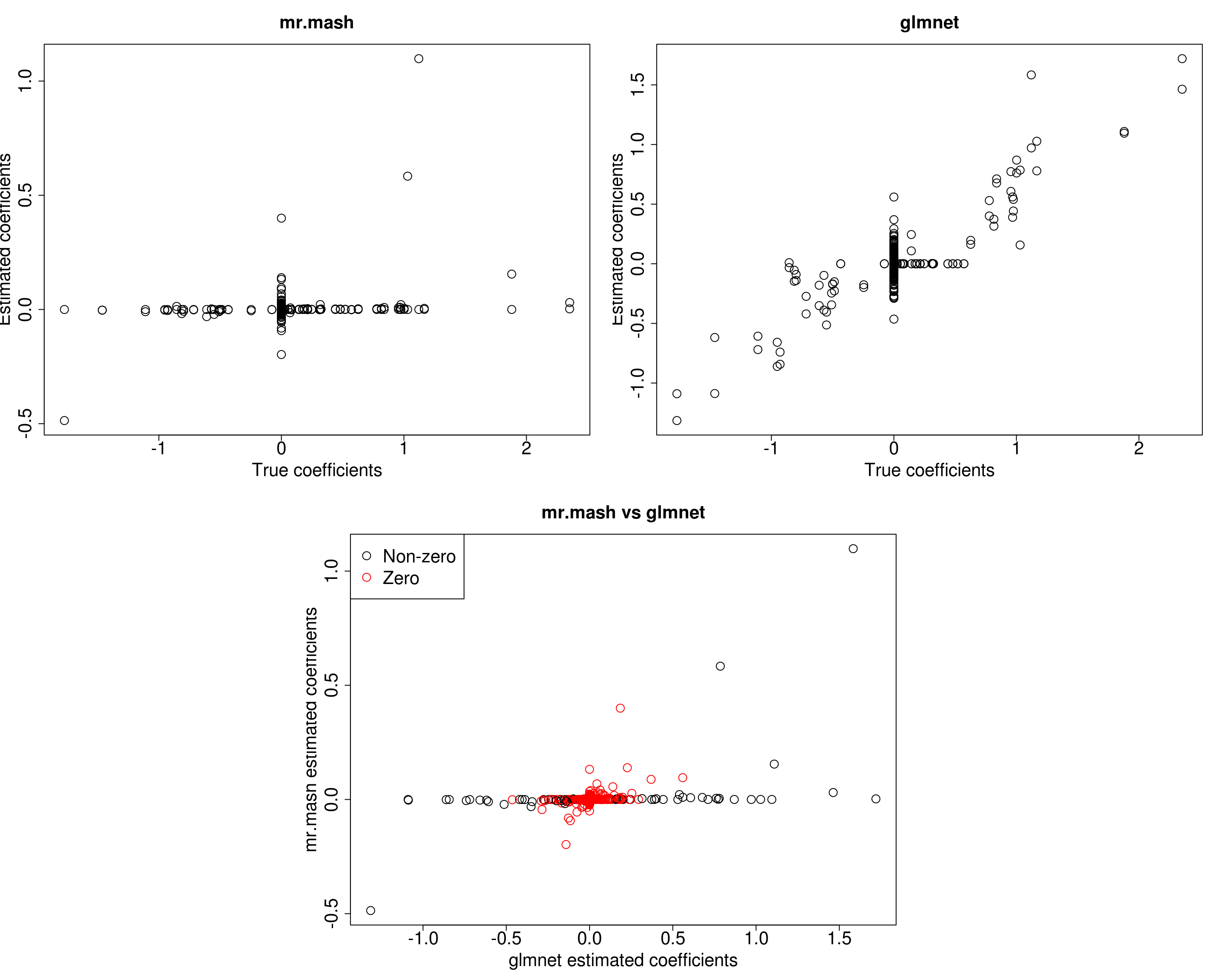
As we can see, mr.mash performs pretty poorly. One possibility is that the prior used cannot capture the pattern of sharing present only among the first two tissues. Let’s now test this hypothesis by adding the correspondent prior matrices to the mixture and re-run mr.mash.
###Update the mixture prior
K <- length(S0)
matr <- matrix(c(1, 1, 0, 0, 0,
                 1, 1, 0, 0, 0,
                 0, 0, 0, 0, 0,
                 0, 0, 0, 0, 0,
                 0, 0, 0, 0, 0), 5, 5, byrow=T)

S0_1 <- S0
for(i in 1:length(grid)){
  S0_1[[K+i]] <- matr * grid[i]
}
print(paste("Length of the original mixture:", K))
[1] "Length of the original mixture: 111"print(paste("Length of the updated mixture:", length(S0_1)))[1] "Length of the updated mixture: 122"###Fit mr.mash
fit_mrmash_updated <- mr.mash(Xtrain, Ytrain, S0_1, update_w0=TRUE, update_w0_method="EM",
compute_ELBO=TRUE, standardize=TRUE, verbose=FALSE, update_V=TRUE,
e=1e-8, ca_update_order="consecutive", mu1_init=Bhat_glmnet)Processing the inputs... Done!
Fitting the optimization algorithm... Done!
Processing the outputs... Done!
mr.mash successfully executed in 5.403984 minutes!Let’s compare the results again.
layout(matrix(c(1, 1, 2, 2,
                1, 1, 2, 2,
                0, 3, 3, 0,
                0, 3, 3, 0), 4, 4, byrow = TRUE))

###Plot estimated vs true coeffcients
##mr.mash
plot(out$B, fit_mrmash_updated$mu1, main="mr.mash", xlab="True coefficients", ylab="Estimated coefficients", cex=2, cex.lab=2, cex.main=2, cex.axis=2)
##glmnet
plot(out$B, Bhat_glmnet, main="glmnet", xlab="True coefficients", ylab="Estimated coefficients",
     cex=2, cex.lab=2, cex.main=2, cex.axis=2)

###Plot mr.mash vs glmnet estimated coeffcients
colorz <- matrix("black", nrow=p, ncol=r)
zeros <- apply(out$B, 2, function(x) x==0)
for(i in 1:ncol(colorz)){
  colorz[zeros[, i], i] <- "red"
}

plot(Bhat_glmnet, fit_mrmash_updated$mu1, main="mr.mash vs glmnet",
     xlab="glmnet estimated coefficients", ylab="mr.mash estimated coefficients",
     col=colorz, cex=2, cex.lab=2, cex.main=2, cex.axis=2)
legend("topleft",
       legend = c("Non-zero", "Zero"),
       col = c("black", "red"),
       pch = c(1, 1),
       horiz = FALSE,
cex=2) 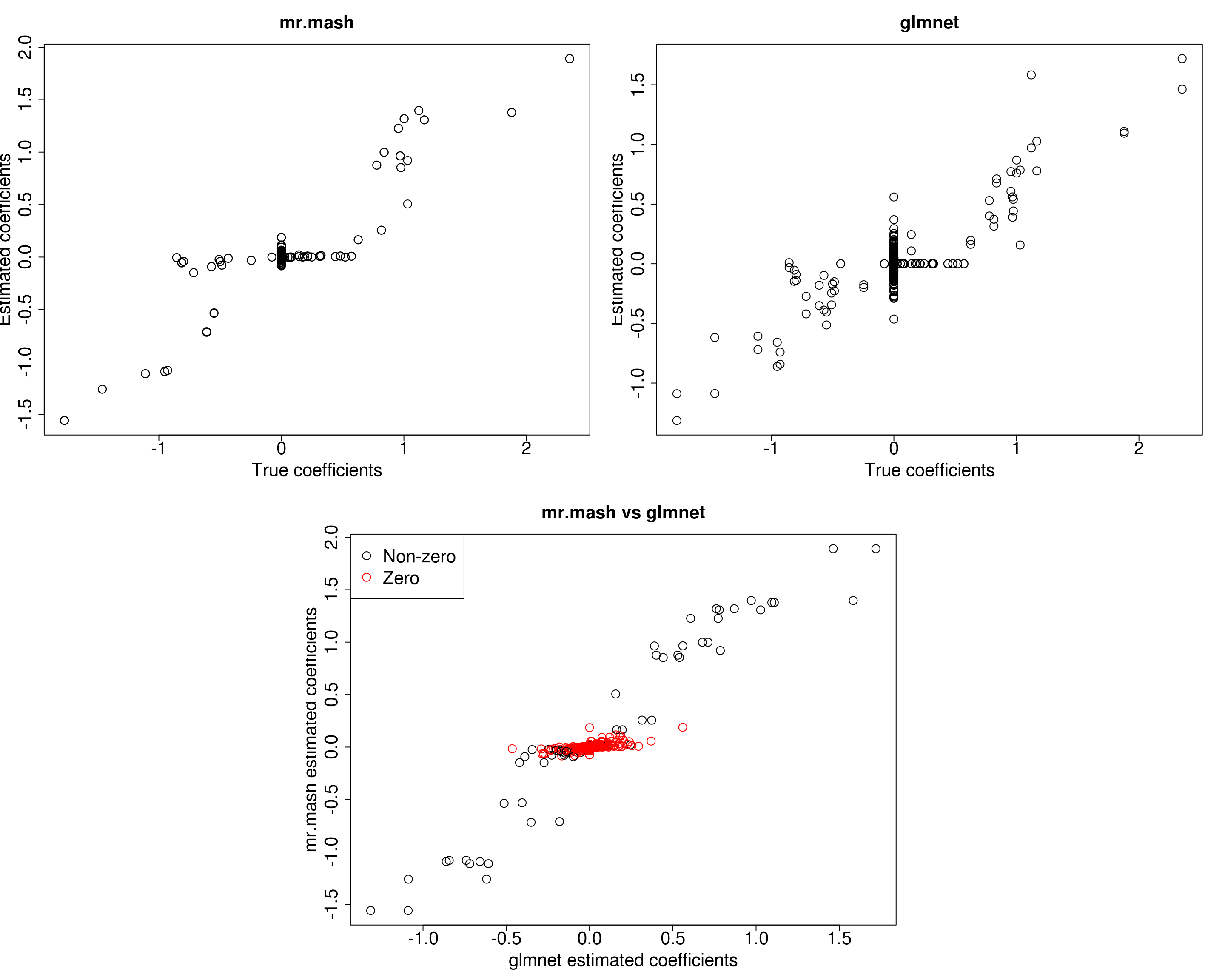
Now the results look much better!
However, we all thought that the identity matrix (properly scaled) should be able to capture these kinds of effects. So, let’s test this intuition by initializing all the parameters (mu1, V, w0) to the true values (keep in mind that these values are from the full data, but we are fitting the model to the training data), updating them, and providing a 2-component prior with the zero matrix and an identity scaled by the true variance (i.e., 0.8).
###Update the mixture prior
zeromat <- matrix(0, r, r)
diagmat <- diag(0.8, r)
S0_2 <- list(S0_1=diagmat, S0_2=zeromat)

###Fit mr.mash
fit_mrmash_diag <- mr.mash(Xtrain, Ytrain, S0_2, w0=c((p_causal/p), (1-(p_causal/p))), V=out$V, mu1_init=out$B,
                          update_w0=TRUE, update_w0_method="EM", compute_ELBO=TRUE, standardize=TRUE,
                          verbose=FALSE, update_V=TRUE, e=1e-8, ca_update_order="consecutive")
Processing the inputs... Done!
Fitting the optimization algorithm... Done!
Processing the outputs... Done!
mr.mash successfully executed in 0.01626393 minutes!###Plot the results
plot(out$B, fit_mrmash_diag$mu1, main="mr.mash", xlab="True coefficients", ylab="Estimated coefficients")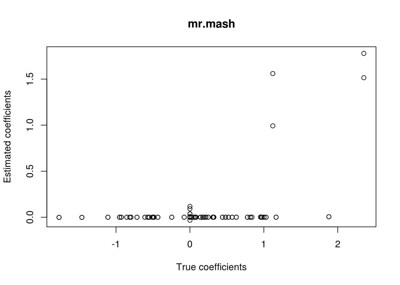
| Version | Author | Date |
|---|---|---|
| 2682eba | fmorgante | 2020-05-28 |
Unfortunately, it does not work well, as we hoped. Let’s now try to fix w0 and V instead of updating them.
###Fit mr.mash
fit_mrmash_diag_fix <- mr.mash(Xtrain, Ytrain, S0_2, w0=c((p_causal/p), (1-(p_causal/p))), V=out$V,
                               mu1_init=out$B, update_w0=FALSE, update_w0_method="EM", compute_ELBO=TRUE,
                               standardize=TRUE, verbose=FALSE, update_V=FALSE, e=1e-8,
                               ca_update_order="consecutive")
Processing the inputs... Done!
Fitting the optimization algorithm... Done!
Processing the outputs... Done!
mr.mash successfully executed in 0.008009799 minutes!###Plot the results
plot(out$B, fit_mrmash_diag_fix$mu1, main="mr.mash", xlab="True coefficients", ylab="Estimated coefficients")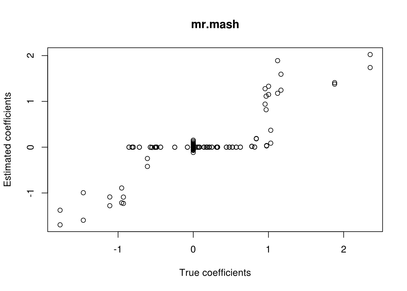
| Version | Author | Date |
|---|---|---|
| 2682eba | fmorgante | 2020-05-28 |
Much better! Now, we will try to update w0 but not V.
###Fit mr.mash
fit_mrmash_diag_fixV <- mr.mash(Xtrain, Ytrain, S0_2, w0=c((p_causal/p), (1-(p_causal/p))), V=out$V,
                               mu1_init=out$B, update_w0=TRUE, update_w0_method="EM", compute_ELBO=TRUE,
                               standardize=TRUE, verbose=FALSE, update_V=FALSE, e=1e-8,
                               ca_update_order="consecutive")
Processing the inputs... Done!
Fitting the optimization algorithm... Done!
Processing the outputs... Done!
mr.mash successfully executed in 0.01221145 minutes!###Plot the results
plot(out$B, fit_mrmash_diag_fixV$mu1, main="mr.mash", xlab="True coefficients", ylab="Estimated coefficients")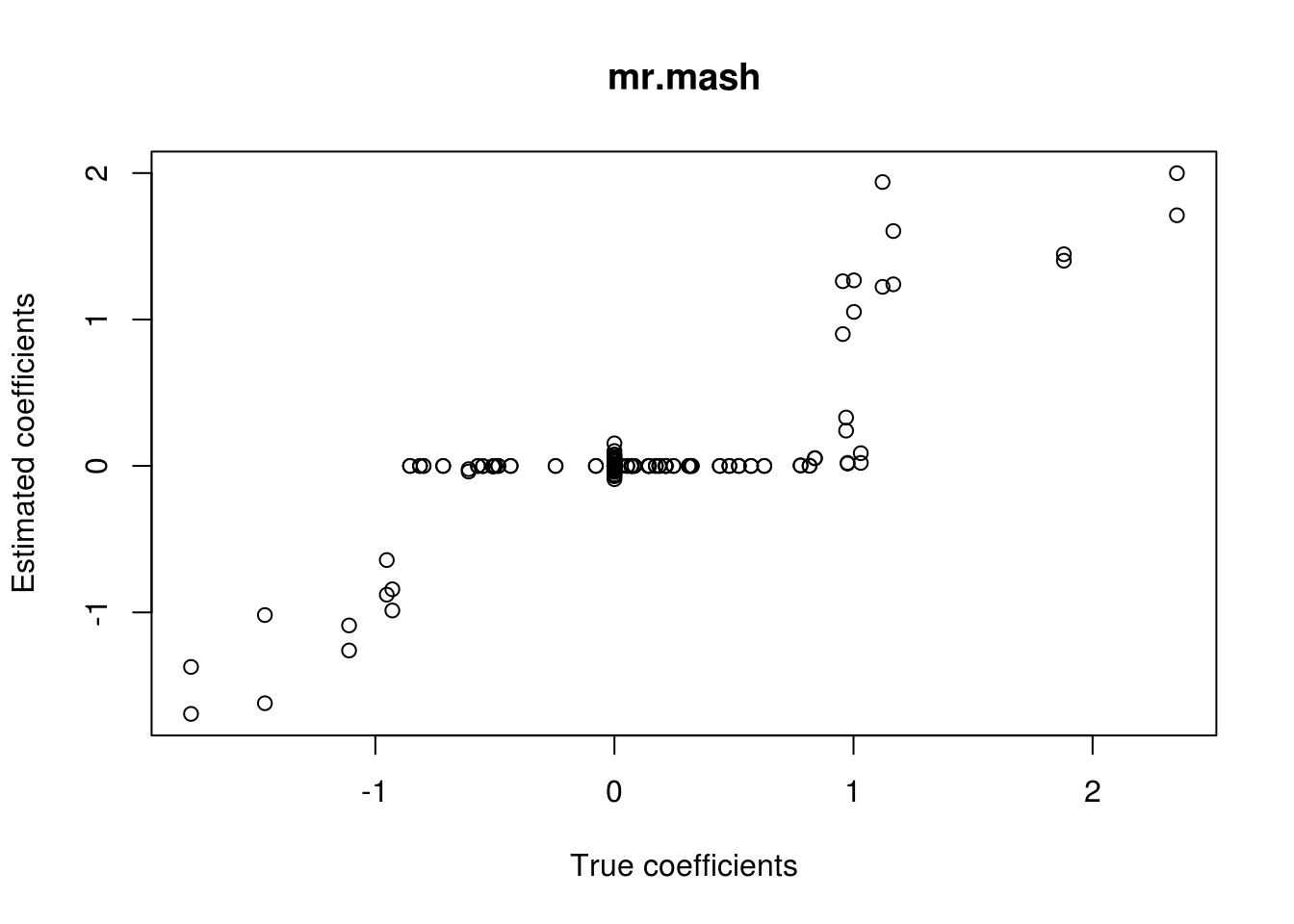
In summary, it looks like the problem is the estimation of V when using an identity matrix to capture this kind of structure in the effects.
print("True V (full data)")[1] "True V (full data)"out$V [,1] [,2] [,3] [,4] [,5]
[1,] 28.0236872 4.2035531 0.7940611 0.7940611 0.7940611
[2,] 4.2035531 28.0236872 0.7940611 0.7940611 0.7940611
[3,] 0.7940611 0.7940611 1.0000000 0.1500000 0.1500000
[4,] 0.7940611 0.7940611 0.1500000 1.0000000 0.1500000
[5,] 0.7940611 0.7940611 0.1500000 0.1500000 1.0000000print("Estimated V from model with the two-component prior with identity (training data)")[1] "Estimated V from model with the two-component prior with identity (training data)"fit_mrmash_diag$V Y1 Y2 Y3 Y4 Y5
Y1 52.9863309 26.2306701 1.0069978 1.10682903 0.40397689
Y2 26.2306701 50.0151618 1.2067022 0.86099911 0.93345668
Y3 1.0069978 1.2067022 1.0283611 0.17562316 0.14786068
Y4 1.1068290 0.8609991 0.1756232 0.92091472 0.09093236
Y5 0.4039769 0.9334567 0.1478607 0.09093236 0.97068662This is not a problem when including the matrix capturing the true structure in the prior.
###Update the mixture prior
zeromat <- matrix(0, r, r)
truemat <- matrix(c(0.8, 0.8, 0, 0, 0,
                     0.8, 0.8, 0, 0, 0,
                     0, 0, 0, 0, 0,
                     0, 0, 0, 0, 0,
                     0, 0, 0, 0, 0), 5, 5, byrow=T)

S0_3 <- list(S0_1=truemat, S0_2=zeromat)

###Fit mr.mash
fit_mrmash_truecov <- mr.mash(Xtrain, Ytrain, S0_3, w0=c((p_causal/p), (1-(p_causal/p))), V=out$V, mu1_init=out$B,
                          update_w0=TRUE, update_w0_method="EM", compute_ELBO=TRUE, standardize=TRUE,
                          verbose=FALSE, update_V=TRUE, e=1e-8, ca_update_order="consecutive")
Processing the inputs... Done!
Fitting the optimization algorithm... Done!
Processing the outputs... Done!
mr.mash successfully executed in 0.01346924 minutes!###Plot the results
plot(out$B, fit_mrmash_truecov$mu1, main="mr.mash", xlab="True coefficients", ylab="Estimated coefficients")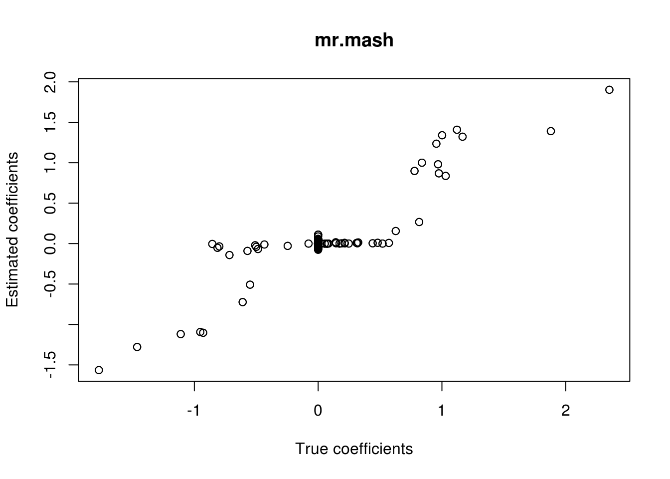
print("True V (full data)")[1] "True V (full data)"out$V [,1] [,2] [,3] [,4] [,5]
[1,] 28.0236872 4.2035531 0.7940611 0.7940611 0.7940611
[2,] 4.2035531 28.0236872 0.7940611 0.7940611 0.7940611
[3,] 0.7940611 0.7940611 1.0000000 0.1500000 0.1500000
[4,] 0.7940611 0.7940611 0.1500000 1.0000000 0.1500000
[5,] 0.7940611 0.7940611 0.1500000 0.1500000 1.0000000print("Estimated V from model with the two-component prior with true effect covariance (training data)")[1] "Estimated V from model with the two-component prior with true effect covariance (training data)"fit_mrmash_truecov$V Y1 Y2 Y3 Y4 Y5
Y1 33.0166995 6.7316366 0.7167243 0.99586720 0.23698598
Y2 6.7316366 31.2216559 0.9371137 0.78008007 0.80928387
Y3 0.7167243 0.9371137 1.0266380 0.17635318 0.15357665
Y4 0.9958672 0.7800801 0.1763532 0.91962359 0.09344052
Y5 0.2369860 0.8092839 0.1535766 0.09344052 0.98858591
sessionInfo()R version 3.5.1 (2018-07-02)
Platform: x86_64-pc-linux-gnu (64-bit)
Running under: Scientific Linux 7.4 (Nitrogen)
Matrix products: default
BLAS/LAPACK: /software/openblas-0.2.19-el7-x86_64/lib/libopenblas_haswellp-r0.2.19.so
locale:
[1] LC_CTYPE=en_US.UTF-8 LC_NUMERIC=C
[3] LC_TIME=en_US.UTF-8 LC_COLLATE=en_US.UTF-8
[5] LC_MONETARY=en_US.UTF-8 LC_MESSAGES=en_US.UTF-8
[7] LC_PAPER=en_US.UTF-8 LC_NAME=C
[9] LC_ADDRESS=C LC_TELEPHONE=C
[11] LC_MEASUREMENT=en_US.UTF-8 LC_IDENTIFICATION=C
attached base packages:
[1] stats graphics grDevices utils datasets methods base
other attached packages:
[1] glmnet_2.0-16 foreach_1.4.4 Matrix_1.2-15
[4] mr.mash.alpha_0.1-74
loaded via a namespace (and not attached):
[1] MBSP_1.0 Rcpp_1.0.4.6 compiler_3.5.1
[4] later_0.7.5 git2r_0.26.1 workflowr_1.6.1
[7] iterators_1.0.10 tools_3.5.1 digest_0.6.25
[10] evaluate_0.12 lattice_0.20-38 GIGrvg_0.5
[13] yaml_2.2.1 SparseM_1.77 mvtnorm_1.0-12
[16] coda_0.19-3 stringr_1.4.0 knitr_1.20
[19] fs_1.3.1 MatrixModels_0.4-1 rprojroot_1.3-2
[22] grid_3.5.1 glue_1.4.0 R6_2.4.1
[25] rmarkdown_1.10 mixsqp_0.3-43 irlba_2.3.3
[28] magrittr_1.5 whisker_0.3-2 codetools_0.2-15
[31] backports_1.1.5 promises_1.0.1 htmltools_0.3.6
[34] matrixStats_0.55.0 mcmc_0.9-6 MASS_7.3-51.1
[37] httpuv_1.4.5 quantreg_5.36 stringi_1.4.3
[40] MCMCpack_1.4-4