Two active responses case - continued
Fabio Morgante
July 02, 2020
Last updated: 2020-07-02
Checks: 7 0
Knit directory: mr_mash_test/
This reproducible R Markdown analysis was created with workflowr (version 1.6.2). The Checks tab describes the reproducibility checks that were applied when the results were created. The Past versions tab lists the development history.
Great! Since the R Markdown file has been committed to the Git repository, you know the exact version of the code that produced these results.
Great job! The global environment was empty. Objects defined in the global environment can affect the analysis in your R Markdown file in unknown ways. For reproduciblity it’s best to always run the code in an empty environment.
The command set.seed(20200328) was run prior to running the code in the R Markdown file. Setting a seed ensures that any results that rely on randomness, e.g. subsampling or permutations, are reproducible.
Great job! Recording the operating system, R version, and package versions is critical for reproducibility.
Nice! There were no cached chunks for this analysis, so you can be confident that you successfully produced the results during this run.
Great job! Using relative paths to the files within your workflowr project makes it easier to run your code on other machines.
Great! You are using Git for version control. Tracking code development and connecting the code version to the results is critical for reproducibility.
The results in this page were generated with repository version 84cf7b9. See the Past versions tab to see a history of the changes made to the R Markdown and HTML files.
Note that you need to be careful to ensure that all relevant files for the analysis have been committed to Git prior to generating the results (you can use wflow_publish or wflow_git_commit). workflowr only checks the R Markdown file, but you know if there are other scripts or data files that it depends on. Below is the status of the Git repository when the results were generated:
Ignored files:
    Ignored:    .sos/
    Ignored:    code/fit_mr_mash.66662433.err
    Ignored:    code/fit_mr_mash.66662433.out
    Ignored:    dsc/.sos/
    Ignored:    dsc/outfiles/
    Ignored:    output/dsc.html
    Ignored:    output/dsc/
    Ignored:    output/dsc_05_18_20.html
    Ignored:    output/dsc_05_18_20/
    Ignored:    output/dsc_05_29_20.html
    Ignored:    output/dsc_05_29_20/
    Ignored:    output/dsc_OLD.html
    Ignored:    output/dsc_OLD/
    Ignored:    output/dsc_test.html
    Ignored:    output/dsc_test/
    Ignored:    output/test_dense_issue.rds
    Ignored:    output/test_sparse_issue.rds

Untracked files:
    Untracked:  analysis/dense_issue_investigation2/
    Untracked:  code/plot_test.R

Unstaged changes:
    Modified:   dsc/midway2.yml
Note that any generated files, e.g. HTML, png, CSS, etc., are not included in this status report because it is ok for generated content to have uncommitted changes.
These are the previous versions of the repository in which changes were made to the R Markdown (analysis/two_active_responses_issue_continued.Rmd) and HTML (docs/two_active_responses_issue_continued.html) files. If you’ve configured a remote Git repository (see ?wflow_git_remote), click on the hyperlinks in the table below to view the files as they were in that past version.
| File | Version | Author | Date | Message |
|---|---|---|---|---|
| Rmd | 84cf7b9 | fmorgante | 2020-07-02 | Fix plot |
| html | c16a043 | fmorgante | 2020-07-02 | Build site. |
| Rmd | fb4c660 | fmorgante | 2020-07-02 | Add two_active_responses_issue_continued results |
library(mr.mash.alpha)
library(glmnet)
Loading required package: MatrixLoading required package: foreachLoaded glmnet 2.0-16###Set options
options(stringsAsFactors = FALSE)
###Functions to compute accuracy and adjusted univariate sumstats
compute_accuracy <- function(Y, Yhat) {
bias <- rep(as.numeric(NA), ncol(Y))
r2 <- rep(as.numeric(NA), ncol(Y))
mse <- rep(as.numeric(NA), ncol(Y))
for(i in 1:ncol(Y)){
fit <- lm(Y[, i] ~ Yhat[, i])
bias[i] <- coef(fit)[2]
r2[i] <- summary(fit)$r.squared
mse[i] <- mean((Y[, i] - Yhat[, i])^2)
}
return(list(bias=bias, r2=r2, mse=mse))
}
compute_univariate_sumstats_adj <- function(X, Y, B, standardize=FALSE, standardize.response=FALSE){
r <- ncol(Y)
p <- ncol(X)
Bhat <- matrix(as.numeric(NA), nrow=p, ncol=r)
Shat <- matrix(as.numeric(NA), nrow=p, ncol=r)
X <- scale(X, center=TRUE, scale=standardize)
Y <- scale(Y, center=TRUE, scale=standardize.response)
if(standardize)
B <- B*attr(X,"scaled:scale")
for(i in 1:r){
for(j in 1:p){
Rij <- Y[, i] - X[, -j]%*%B[-j, i]
fit <- lm(Rij ~ X[, j]-1)
Bhat[j, i] <- coef(fit)
Shat[j, i] <- summary(fit)$coefficients[1, 2]
}
}
return(list(Bhat=Bhat, Shat=Shat))
}We simulate data with n=600, p=1,000, p_causal=50, r=6, PVE=0.5, 2 causal responses with shared effects, independent predictors, and independent residuals. The models will be fitted to the training data (80% of the full data), and .
###Set seed
set.seed(123)
###Set parameters
n <- 600
p <- 1000
p_causal <- 50
r <- 6
r_causal <- list(1:2)
B_cor <- 1
B_scale <- 1
w <- 1

###Simulate V, B, X and Y
out <- simulate_mr_mash_data(n, p, p_causal, r, r_causal, intercepts = rep(1, r),
                            pve=0.5, B_cor=B_cor, B_scale=B_scale, w=w,
                            X_cor=0, X_scale=1, V_cor=0)
colnames(out$Y) <- paste0("Y", seq(1, r))
rownames(out$Y) <- paste0("N", seq(1, n))
colnames(out$X) <- paste0("X", seq(1, p))
rownames(out$X) <- paste0("N", seq(1, n))

###Split the data in training and test sets
test_set <- sort(sample(x=c(1:n), size=round(n*0.2), replace=FALSE))
Ytrain <- out$Y[-test_set, ]
Xtrain <- out$X[-test_set, ]
Ytest <- out$Y[test_set, ]
Xtest <- out$X[test_set, ]
We build the mixture prior as usual including zero matrix, identity matrix, rank-1 matrices, and shared matrix, each scaled by a grid computed from univariate summary statistics.
###Compute grid of variances
univ_sumstats <- compute_univariate_sumstats(Xtrain, Ytrain, standardize=FALSE, standardize.response=FALSE)
grid <- autoselect.mixsd(univ_sumstats, mult=sqrt(2))^2

###Compute prior with only canonical matrices
S0_can <- compute_canonical_covs(ncol(Ytrain), singletons=TRUE, hetgrid=c(0, 0.5, 1))
S0 <- expand_covs(S0_can, grid, zeromat=TRUE)
We run glmnet with \(\alpha=1\) to obtain an inital estimate for the regression coefficients to provide to mr.mash, and for comparison.
###Fit grop-lasso to initialize mr.mash
cvfit_glmnet <- cv.glmnet(x=Xtrain, y=Ytrain, family="mgaussian", alpha=1, standardize=FALSE)
coeff_glmnet <- coef(cvfit_glmnet, s="lambda.min")
Bhat_glmnet <- matrix(as.numeric(NA), nrow=p, ncol=r)
for(i in 1:length(coeff_glmnet)){
  Bhat_glmnet[, i] <- as.vector(coeff_glmnet[[i]])[-1]
}
Yhat_glmnet <- drop(predict(cvfit_glmnet, newx=Xtest, s="lambda.min"))
prop_nonzero_glmnet <- sum(Bhat_glmnet[, 1]!=0)/p
We run mr.mash with EM updates of the mixture weights, updating V (imposing a diagonal structure), and initializing the regression coefficients with the estimates from glmnet.
w0 <- c((1-prop_nonzero_glmnet), rep(prop_nonzero_glmnet/(length(S0)-1), (length(S0)-1)))
fit_mrmash <- mr.mash(Xtrain, Ytrain, S0, w0=w0, update_w0=TRUE, update_w0_method="EM", tol=1e-2,
                      convergence_criterion="ELBO", compute_ELBO=TRUE, standardize=FALSE,
                      verbose=FALSE, update_V=TRUE, update_V_method="diagonal", e=1e-8,
                      mu1_init=Bhat_glmnet, w0_threshold=0)
Yhat_mrmash <- predict(fit_mrmash, Xtest)
We now compare the results.
layout(matrix(c(1, 1, 2, 2,
                1, 1, 2, 2,
                0, 3, 3, 0,
                0, 3, 3, 0), 4, 4, byrow = TRUE))

###Plot estimated vs true coeffcients
##mr.mash
plot(out$B, fit_mrmash$mu1, main="mr.mash", xlab="True coefficients", ylab="Estimated coefficients",
     cex=2, cex.lab=2, cex.main=2, cex.axis=2)
##glmnet
plot(out$B, Bhat_glmnet, main="glmnet", xlab="True coefficients", ylab="Estimated coefficients",
     cex=2, cex.lab=2, cex.main=2, cex.axis=2)

###Plot mr.mash vs glmnet estimated coeffcients
colorz <- matrix("black", nrow=p, ncol=r)
zeros <- apply(out$B, 2, function(x) x==0)
for(i in 1:ncol(colorz)){
  colorz[zeros[, i], i] <- "red"
}

plot(Bhat_glmnet, fit_mrmash$mu1, main="mr.mash vs glmnet",
     xlab="glmnet estimated coefficients", ylab="mr.mash estimated coefficients",
     col=colorz, cex=2, cex.lab=2, cex.main=2, cex.axis=2)
legend("topleft",
       legend = c("Non-zero", "Zero"),
       col = c("black", "red"),
       pch = c(1, 1),
       horiz = FALSE,
cex=2) 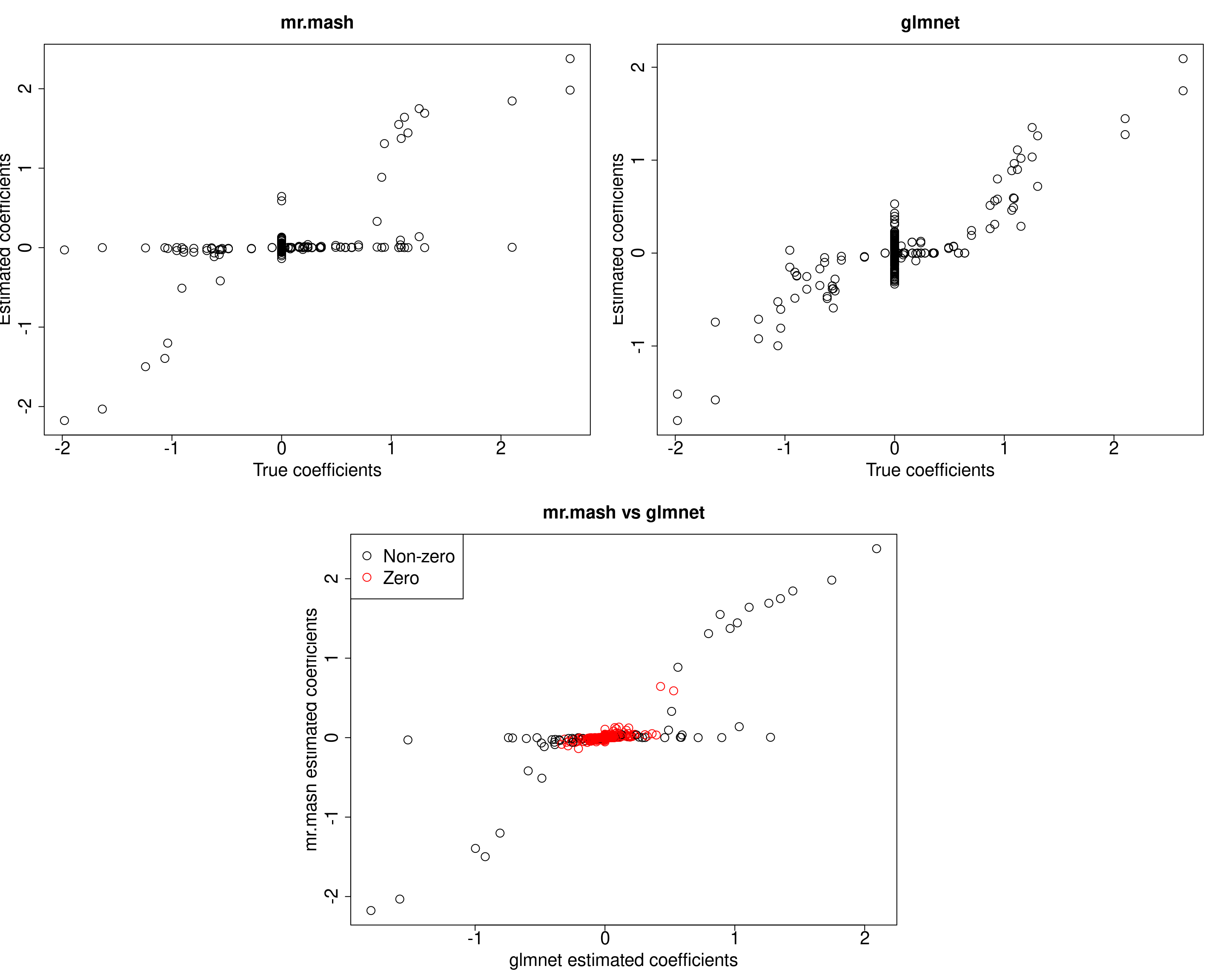
| Version | Author | Date |
|---|---|---|
| c16a043 | fmorgante | 2020-07-02 |
cat("Prediction MSE of glmnet\n")Prediction MSE of glmnetcompute_accuracy(Ytest, Yhat_glmnet)$mse[1] 51.0744117 59.5319506 1.0282797 0.9160763 1.0676336 1.1469770cat("Prediction MSE of mr.mash\n")Prediction MSE of mr.mashcompute_accuracy(Ytest, Yhat_mrmash)$mse[1] 59.8435334 79.1757052 0.9611462 0.8985343 1.0179589 1.1145080As we can see, mr.mash performs pretty poorly.
Let’s now try to repeate the simulation above but with 4 causal reponses with shared effects.
###Set seed
set.seed(123)
###Set parameters
n <- 600
p <- 1000
p_causal <- 50
r <- 6
r_causal <- list(1:4)
B_cor <- 1
B_scale <- 1
w <- 1

###Simulate V, B, X and Y
out <- simulate_mr_mash_data(n, p, p_causal, r, r_causal, intercepts = rep(1, r),
                            pve=0.5, B_cor=B_cor, B_scale=B_scale, w=w,
                            X_cor=0, X_scale=1, V_cor=0)
colnames(out$Y) <- paste0("Y", seq(1, r))
rownames(out$Y) <- paste0("N", seq(1, n))
colnames(out$X) <- paste0("X", seq(1, p))
rownames(out$X) <- paste0("N", seq(1, n))

###Split the data in training and test sets
test_set <- sort(sample(x=c(1:n), size=round(n*0.2), replace=FALSE))
Ytrain <- out$Y[-test_set, ]
Xtrain <- out$X[-test_set, ]
Ytest <- out$Y[test_set, ]
Xtest <- out$X[test_set, ]

###Compute grid of variances
univ_sumstats <- compute_univariate_sumstats(Xtrain, Ytrain, standardize=FALSE, standardize.response=FALSE)
grid <- autoselect.mixsd(univ_sumstats, mult=sqrt(2))^2

###Compute prior with only canonical matrices
S0_can <- compute_canonical_covs(ncol(Ytrain), singletons=TRUE, hetgrid=c(0, 0.5, 1))
S0 <- expand_covs(S0_can, grid, zeromat=TRUE)

###Fit grop-lasso to initialize mr.mash
cvfit_glmnet <- cv.glmnet(x=Xtrain, y=Ytrain, family="mgaussian", alpha=1, standardize=FALSE)
coeff_glmnet <- coef(cvfit_glmnet, s="lambda.min")
Bhat_glmnet <- matrix(as.numeric(NA), nrow=p, ncol=r)
for(i in 1:length(coeff_glmnet)){
  Bhat_glmnet[, i] <- as.vector(coeff_glmnet[[i]])[-1]
}
Yhat_glmnet <- drop(predict(cvfit_glmnet, newx=Xtest, s="lambda.min"))
prop_nonzero_glmnet <- sum(Bhat_glmnet[, 1]!=0)/p

###Fit mr.mash
w0 <- c((1-prop_nonzero_glmnet), rep(prop_nonzero_glmnet/(length(S0)-1), (length(S0)-1)))
fit_mrmash <- mr.mash(Xtrain, Ytrain, S0, w0=w0, update_w0=TRUE, update_w0_method="EM", tol=1e-2,
                      convergence_criterion="ELBO", compute_ELBO=TRUE, standardize=FALSE,
                      verbose=FALSE, update_V=TRUE, update_V_method="diagonal", e=1e-8,
                      mu1_init=Bhat_glmnet, w0_threshold=0)
Processing the inputs... Done!
Fitting the optimization algorithm... Done!
Processing the outputs... Done!
mr.mash successfully executed in 1.024651 minutes!Yhat_mrmash <- predict(fit_mrmash, Xtest)
layout(matrix(c(1, 1, 2, 2,
1, 1, 2, 2,
0, 3, 3, 0,
0, 3, 3, 0), 4, 4, byrow = TRUE))
###Plot estimated vs true coeffcients
##mr.mash
plot(out$B, fit_mrmash$mu1, main="mr.mash", xlab="True coefficients", ylab="Estimated coefficients",
cex=2, cex.lab=2, cex.main=2, cex.axis=2)
##glmnet
plot(out$B, Bhat_glmnet, main="glmnet", xlab="True coefficients", ylab="Estimated coefficients",
cex=2, cex.lab=2, cex.main=2, cex.axis=2)
###Plot mr.mash vs glmnet estimated coeffcients
colorz <- matrix("black", nrow=p, ncol=r)
zeros <- apply(out$B, 2, function(x) x==0)
for(i in 1:ncol(colorz)){
colorz[zeros[, i], i] <- "red"
}
plot(Bhat_glmnet, fit_mrmash$mu1, main="mr.mash vs glmnet",
xlab="glmnet estimated coefficients", ylab="mr.mash estimated coefficients",
col=colorz, cex=2, cex.lab=2, cex.main=2, cex.axis=2)
legend("topleft",
legend = c("Non-zero", "Zero"),
col = c("black", "red"),
pch = c(1, 1),
horiz = FALSE,
cex=2) 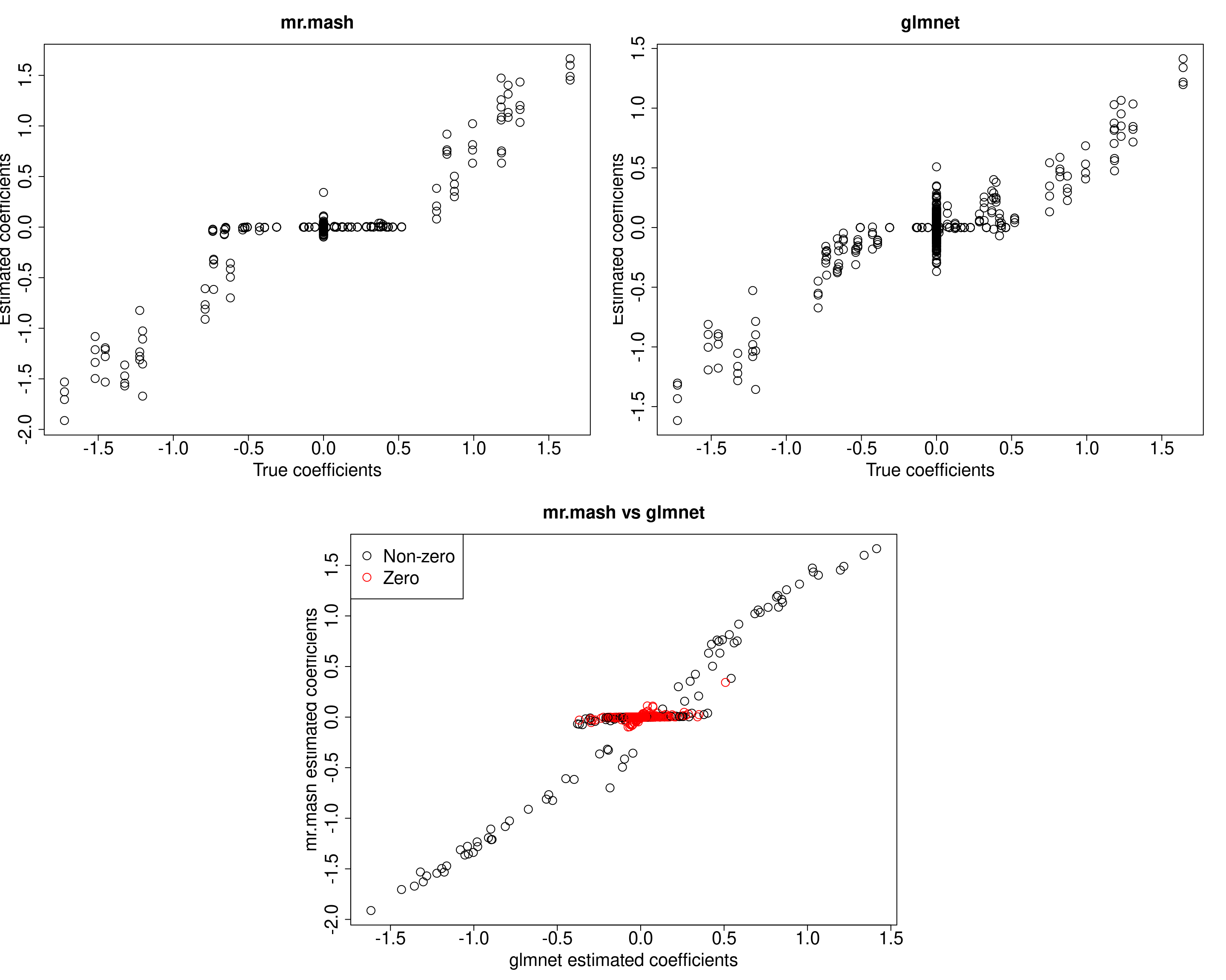
| Version | Author | Date |
|---|---|---|
| c16a043 | fmorgante | 2020-07-02 |
cat("Prediction MSE of glmnet\n")Prediction MSE of glmnetcompute_accuracy(Ytest, Yhat_glmnet)$mse[1] 38.610514 32.189724 43.038023 37.286888 1.137985 1.046656cat("Prediction MSE of mr.mash\n")Prediction MSE of mr.mashcompute_accuracy(Ytest, Yhat_mrmash)$mse[1] 38.428774 30.717547 40.571693 33.805393 1.110894 1.040049Here, we can see that mr.mash performs better.
We will now see what happens if repeate the analysis above but with 2 groups of 2 causal reponses with shared effects and a group of 2 responses with no effect. The variables come from each of the two mixture components with equal probability.
###Set seed
set.seed(123)
###Set parameters
n <- 600
p <- 1000
p_causal <- 50
r <- 6
r_causal <- list(1:2, 3:4)
B_cor <- c(1, 1)
B_scale <- c(1, 1)
w <- c(0.5, 0.5)

###Simulate V, B, X and Y
out <- simulate_mr_mash_data(n, p, p_causal, r, r_causal, intercepts = rep(1, r),
                            pve=0.5, B_cor=B_cor, B_scale=B_scale, w=w,
                            X_cor=0, X_scale=1, V_cor=0)
colnames(out$Y) <- paste0("Y", seq(1, r))
rownames(out$Y) <- paste0("N", seq(1, n))
colnames(out$X) <- paste0("X", seq(1, p))
rownames(out$X) <- paste0("N", seq(1, n))

###Split the data in training and test sets
test_set <- sort(sample(x=c(1:n), size=round(n*0.2), replace=FALSE))
Ytrain <- out$Y[-test_set, ]
Xtrain <- out$X[-test_set, ]
Ytest <- out$Y[test_set, ]
Xtest <- out$X[test_set, ]

###Compute grid of variances
univ_sumstats <- compute_univariate_sumstats(Xtrain, Ytrain, standardize=FALSE, standardize.response=FALSE)
grid <- autoselect.mixsd(univ_sumstats, mult=sqrt(2))^2

###Compute prior with only canonical matrices
S0_can <- compute_canonical_covs(ncol(Ytrain), singletons=TRUE, hetgrid=c(0, 0.5, 1))
S0 <- expand_covs(S0_can, grid, zeromat=TRUE)

###Fit grop-lasso to initialize mr.mash
cvfit_glmnet <- cv.glmnet(x=Xtrain, y=Ytrain, family="mgaussian", alpha=1, standardize=FALSE)
coeff_glmnet <- coef(cvfit_glmnet, s="lambda.min")
Bhat_glmnet <- matrix(as.numeric(NA), nrow=p, ncol=r)
for(i in 1:length(coeff_glmnet)){
  Bhat_glmnet[, i] <- as.vector(coeff_glmnet[[i]])[-1]
}
Yhat_glmnet <- drop(predict(cvfit_glmnet, newx=Xtest, s="lambda.min"))
prop_nonzero_glmnet <- sum(Bhat_glmnet[, 1]!=0)/p

###Fit mr.mash
w0 <- c((1-prop_nonzero_glmnet), rep(prop_nonzero_glmnet/(length(S0)-1), (length(S0)-1)))
fit_mrmash <- mr.mash(Xtrain, Ytrain, S0, w0=w0, update_w0=TRUE, update_w0_method="EM", tol=1e-2,
                      convergence_criterion="ELBO", compute_ELBO=TRUE, standardize=FALSE,
                      verbose=FALSE, update_V=TRUE, update_V_method="diagonal", e=1e-8,
                      mu1_init=Bhat_glmnet, w0_threshold=0)
Processing the inputs... Done!
Fitting the optimization algorithm... Done!
Processing the outputs... Done!
mr.mash successfully executed in 1.803128 minutes!Yhat_mrmash <- predict(fit_mrmash, Xtest)
layout(matrix(c(1, 1, 2, 2,
1, 1, 2, 2,
0, 3, 3, 0,
0, 3, 3, 0), 4, 4, byrow = TRUE))
###Plot estimated vs true coeffcients
##mr.mash
plot(out$B, fit_mrmash$mu1, main="mr.mash", xlab="True coefficients", ylab="Estimated coefficients",
cex=2, cex.lab=2, cex.main=2, cex.axis=2)
##glmnet
plot(out$B, Bhat_glmnet, main="glmnet", xlab="True coefficients", ylab="Estimated coefficients",
cex=2, cex.lab=2, cex.main=2, cex.axis=2)
###Plot mr.mash vs glmnet estimated coeffcients
colorz <- matrix("black", nrow=p, ncol=r)
zeros <- apply(out$B, 2, function(x) x==0)
for(i in 1:ncol(colorz)){
colorz[zeros[, i], i] <- "red"
}
plot(Bhat_glmnet, fit_mrmash$mu1, main="mr.mash vs glmnet",
xlab="glmnet estimated coefficients", ylab="mr.mash estimated coefficients",
col=colorz, cex=2, cex.lab=2, cex.main=2, cex.axis=2)
legend("topleft",
legend = c("Non-zero", "Zero"),
col = c("black", "red"),
pch = c(1, 1),
horiz = FALSE,
cex=2) 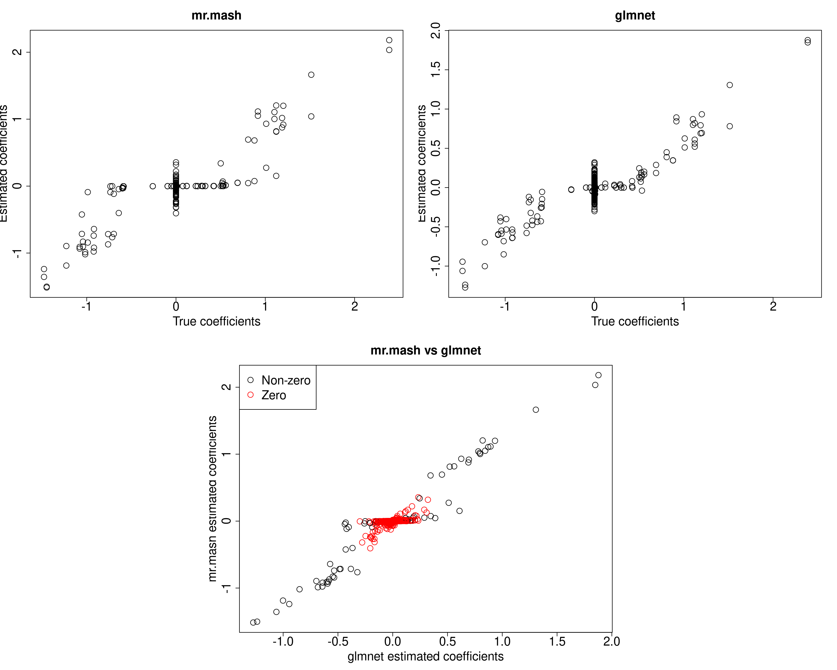
| Version | Author | Date |
|---|---|---|
| c16a043 | fmorgante | 2020-07-02 |
cat("Prediction MSE of glmnet\n")Prediction MSE of glmnetcompute_accuracy(Ytest, Yhat_glmnet)$mse[1] 17.287026 20.098277 26.707034 21.409663 1.100715 1.134953cat("Prediction MSE of mr.mash\n")Prediction MSE of mr.mashcompute_accuracy(Ytest, Yhat_mrmash)$mse[1] 16.066425 18.771813 28.913112 19.365426 1.110864 1.113349Surprisingly, mr.mash seems to do pretty well in this situation too.
sessionInfo()R version 3.5.1 (2018-07-02)
Platform: x86_64-pc-linux-gnu (64-bit)
Running under: Scientific Linux 7.4 (Nitrogen)
Matrix products: default
BLAS/LAPACK: /software/openblas-0.2.19-el7-x86_64/lib/libopenblas_haswellp-r0.2.19.so
locale:
[1] LC_CTYPE=en_US.UTF-8 LC_NUMERIC=C
[3] LC_TIME=en_US.UTF-8 LC_COLLATE=en_US.UTF-8
[5] LC_MONETARY=en_US.UTF-8 LC_MESSAGES=en_US.UTF-8
[7] LC_PAPER=en_US.UTF-8 LC_NAME=C
[9] LC_ADDRESS=C LC_TELEPHONE=C
[11] LC_MEASUREMENT=en_US.UTF-8 LC_IDENTIFICATION=C
attached base packages:
[1] stats graphics grDevices utils datasets methods base
other attached packages:
[1] glmnet_2.0-16 foreach_1.4.4 Matrix_1.2-15
[4] mr.mash.alpha_0.1-96
loaded via a namespace (and not attached):
[1] MBSP_1.0 Rcpp_1.0.4.6 plyr_1.8.6
[4] compiler_3.5.1 mashr_0.2.38 later_0.7.5
[7] git2r_0.26.1 workflowr_1.6.2 iterators_1.0.10
[10] tools_3.5.1 digest_0.6.25 evaluate_0.14
[13] lattice_0.20-38 GIGrvg_0.5 yaml_2.2.1
[16] mvtnorm_1.1-1 SparseM_1.77 invgamma_1.1
[19] coda_0.19-3 stringr_1.4.0 knitr_1.20
[22] fs_1.3.1 MatrixModels_0.4-1 rprojroot_1.3-2
[25] grid_3.5.1 glue_1.4.1 R6_2.4.1
[28] rmarkdown_1.10 mixsqp_0.3-44 rmeta_3.0
[31] irlba_2.3.3 ashr_2.2-50 magrittr_1.5
[34] whisker_0.3-2 codetools_0.2-15 matrixStats_0.56.0
[37] backports_1.1.8 promises_1.0.1 htmltools_0.3.6
[40] mcmc_0.9-6 MASS_7.3-51.1 assertthat_0.2.1
[43] abind_1.4-5 httpuv_1.4.5 quantreg_5.36
[46] stringi_1.4.6 MCMCpack_1.4-4 truncnorm_1.0-8
[49] SQUAREM_2020.3