Effects structure similar to GTEx
Fabio Morgante
September 29, 2020
Last updated: 2020-09-29
Checks: 7 0
Knit directory: mr_mash_test/
This reproducible R Markdown analysis was created with workflowr (version 1.6.2). The Checks tab describes the reproducibility checks that were applied when the results were created. The Past versions tab lists the development history.
Great! Since the R Markdown file has been committed to the Git repository, you know the exact version of the code that produced these results.
Great job! The global environment was empty. Objects defined in the global environment can affect the analysis in your R Markdown file in unknown ways. For reproduciblity it’s best to always run the code in an empty environment.
The command set.seed(20200328) was run prior to running the code in the R Markdown file. Setting a seed ensures that any results that rely on randomness, e.g. subsampling or permutations, are reproducible.
Great job! Recording the operating system, R version, and package versions is critical for reproducibility.
Nice! There were no cached chunks for this analysis, so you can be confident that you successfully produced the results during this run.
Great job! Using relative paths to the files within your workflowr project makes it easier to run your code on other machines.
Great! You are using Git for version control. Tracking code development and connecting the code version to the results is critical for reproducibility.
The results in this page were generated with repository version fab8dab. See the Past versions tab to see a history of the changes made to the R Markdown and HTML files.
Note that you need to be careful to ensure that all relevant files for the analysis have been committed to Git prior to generating the results (you can use wflow_publish or wflow_git_commit). workflowr only checks the R Markdown file, but you know if there are other scripts or data files that it depends on. Below is the status of the Git repository when the results were generated:
Ignored files:
    Ignored:    .sos/
    Ignored:    code/assess_mrmash_speed.2835257.err
    Ignored:    code/assess_mrmash_speed.2835257.out
    Ignored:    code/assess_mrmash_speed.2914525.err
    Ignored:    code/assess_mrmash_speed.2914525.out
    Ignored:    code/fit_mr_mash.66662433.err
    Ignored:    code/fit_mr_mash.66662433.out
    Ignored:    dsc/.sos/
    Ignored:    dsc/dsc_mvreg_07_29_20.3339807.err
    Ignored:    dsc/dsc_mvreg_07_29_20.3339807.out
    Ignored:    dsc/dsc_mvreg_07_29_20.3340460.err
    Ignored:    dsc/dsc_mvreg_07_29_20.3340460.out
    Ignored:    dsc/dsc_mvreg_07_29_20.3341113.err
    Ignored:    dsc/dsc_mvreg_07_29_20.3341113.out
    Ignored:    dsc/dsc_mvreg_07_29_20.3352804.err
    Ignored:    dsc/dsc_mvreg_07_29_20.3352804.out
    Ignored:    dsc/outfiles/
    Ignored:    output/dsc.html
    Ignored:    output/dsc/
    Ignored:    output/dsc_05_18_20.html
    Ignored:    output/dsc_05_18_20/
    Ignored:    output/dsc_07_29_20.html
    Ignored:    output/dsc_07_29_20/
    Ignored:    output/dsc_OLD.html
    Ignored:    output/dsc_OLD/
    Ignored:    output/dsc_test.html
    Ignored:    output/dsc_test/
    Ignored:    output/dsc_test_inter/
    Ignored:    output/mvreg_all_genes_prior_corrX_indepV_sharedB_2blocksr10.html
    Ignored:    output/mvreg_all_genes_prior_corrX_indepV_sharedB_2blocksr10/
    Ignored:    output/mvreg_all_genes_prior_corrX_indepV_sharedB_2blocksr10_inter/
    Ignored:    output/mvreg_all_genes_prior_highcorrX_indepV_sharedB_2blocksr10.html
    Ignored:    output/mvreg_all_genes_prior_highcorrX_indepV_sharedB_2blocksr10/
    Ignored:    output/mvreg_all_genes_prior_highcorrX_indepV_sharedB_2blocksr10_inter/
    Ignored:    output/mvreg_all_genes_prior_indepX_indepV_sharedB_2blocksr10.html
    Ignored:    output/mvreg_all_genes_prior_indepX_indepV_sharedB_2blocksr10/
    Ignored:    output/mvreg_all_genes_prior_indepX_indepV_sharedB_2blocksr10_inter/
    Ignored:    output/mvreg_all_genes_prior_indepX_indepV_sharedB_2blocksr10_test.html
    Ignored:    output/mvreg_all_genes_prior_indepX_indepV_sharedB_2blocksr10_test/
    Ignored:    output/mvreg_all_genes_prior_indepX_indepV_sharedB_2blocksr10_test_inter/
    Ignored:    output/mvreg_all_genes_prior_indepX_indepV_sharedB_3causalrespr10.html
    Ignored:    output/mvreg_all_genes_prior_indepX_indepV_sharedB_3causalrespr10/
    Ignored:    output/mvreg_all_genes_prior_indepX_indepV_sharedB_3causalrespr10_inter/
    Ignored:    output/test_dense_issue.rds
    Ignored:    output/test_sparse_issue.rds
    Ignored:    scripts/.sos/
    Ignored:    scripts/mvreg_all_genes_prior_corrX_indepV_sharedB_2blocksr10_pipeline.5297178.err
    Ignored:    scripts/mvreg_all_genes_prior_corrX_indepV_sharedB_2blocksr10_pipeline.5297178.out
    Ignored:    scripts/mvreg_all_genes_prior_corrX_indepV_sharedB_2blocksr10_pipeline.5297184.err
    Ignored:    scripts/mvreg_all_genes_prior_corrX_indepV_sharedB_2blocksr10_pipeline.5297184.out
    Ignored:    scripts/mvreg_all_genes_prior_corrX_indepV_sharedB_2blocksr10_pipeline.5299552.err
    Ignored:    scripts/mvreg_all_genes_prior_corrX_indepV_sharedB_2blocksr10_pipeline.5299552.out
    Ignored:    scripts/mvreg_all_genes_prior_corrX_indepV_sharedB_2blocksr10_pipeline.5300596.err
    Ignored:    scripts/mvreg_all_genes_prior_corrX_indepV_sharedB_2blocksr10_pipeline.5300596.out
    Ignored:    scripts/mvreg_all_genes_prior_corrX_indepV_sharedB_2blocksr10_pipeline.5300796.err
    Ignored:    scripts/mvreg_all_genes_prior_corrX_indepV_sharedB_2blocksr10_pipeline.5300796.out
    Ignored:    scripts/mvreg_all_genes_prior_highcorrX_indepV_sharedB_2blocksr10_pipeline.5305725.err
    Ignored:    scripts/mvreg_all_genes_prior_highcorrX_indepV_sharedB_2blocksr10_pipeline.5305725.out
    Ignored:    scripts/mvreg_all_genes_prior_highcorrX_indepV_sharedB_2blocksr10_pipeline.5305727.err
    Ignored:    scripts/mvreg_all_genes_prior_highcorrX_indepV_sharedB_2blocksr10_pipeline.5305727.out
    Ignored:    scripts/mvreg_all_genes_prior_highcorrX_indepV_sharedB_2blocksr10_pipeline.5308354.err
    Ignored:    scripts/mvreg_all_genes_prior_highcorrX_indepV_sharedB_2blocksr10_pipeline.5308354.out
    Ignored:    scripts/mvreg_all_genes_prior_highcorrX_indepV_sharedB_2blocksr10_pipeline.5309181.err
    Ignored:    scripts/mvreg_all_genes_prior_highcorrX_indepV_sharedB_2blocksr10_pipeline.5309181.out
    Ignored:    scripts/mvreg_all_genes_prior_highcorrX_indepV_sharedB_2blocksr10_pipeline.5310380.err
    Ignored:    scripts/mvreg_all_genes_prior_highcorrX_indepV_sharedB_2blocksr10_pipeline.5310380.out
    Ignored:    scripts/mvreg_all_genes_prior_indepX_indepV_sharedB_2blocksr10_pipeline.5290364.err
    Ignored:    scripts/mvreg_all_genes_prior_indepX_indepV_sharedB_2blocksr10_pipeline.5290364.out
    Ignored:    scripts/mvreg_all_genes_prior_indepX_indepV_sharedB_2blocksr10_pipeline.5290365.err
    Ignored:    scripts/mvreg_all_genes_prior_indepX_indepV_sharedB_2blocksr10_pipeline.5290365.out
    Ignored:    scripts/mvreg_all_genes_prior_indepX_indepV_sharedB_2blocksr10_pipeline.5293048.err
    Ignored:    scripts/mvreg_all_genes_prior_indepX_indepV_sharedB_2blocksr10_pipeline.5293048.out
    Ignored:    scripts/mvreg_all_genes_prior_indepX_indepV_sharedB_2blocksr10_pipeline.5294079.err
    Ignored:    scripts/mvreg_all_genes_prior_indepX_indepV_sharedB_2blocksr10_pipeline.5294079.out
    Ignored:    scripts/mvreg_all_genes_prior_indepX_indepV_sharedB_2blocksr10_pipeline.5295637.err
    Ignored:    scripts/mvreg_all_genes_prior_indepX_indepV_sharedB_2blocksr10_pipeline.5295637.out
    Ignored:    scripts/mvreg_all_genes_prior_indepX_indepV_sharedB_2blocksr10_pipeline.5297100.err
    Ignored:    scripts/mvreg_all_genes_prior_indepX_indepV_sharedB_2blocksr10_pipeline.5297100.out
    Ignored:    scripts/mvreg_all_genes_prior_indepX_indepV_sharedB_3causalrespr10_pipeline.5315542.err
    Ignored:    scripts/mvreg_all_genes_prior_indepX_indepV_sharedB_3causalrespr10_pipeline.5315542.out
    Ignored:    scripts/mvreg_all_genes_prior_indepX_indepV_sharedB_3causalrespr10_pipeline.5315575.err
    Ignored:    scripts/mvreg_all_genes_prior_indepX_indepV_sharedB_3causalrespr10_pipeline.5315575.out
    Ignored:    scripts/mvreg_all_genes_prior_indepX_indepV_sharedB_3causalrespr10_pipeline.5318936.err
    Ignored:    scripts/mvreg_all_genes_prior_indepX_indepV_sharedB_3causalrespr10_pipeline.5318936.out
    Ignored:    scripts/mvreg_all_genes_prior_indepX_indepV_sharedB_3causalrespr10_pipeline.5374687.err
    Ignored:    scripts/mvreg_all_genes_prior_indepX_indepV_sharedB_3causalrespr10_pipeline.5374687.out
    Ignored:    scripts/mvreg_all_genes_prior_indepX_indepV_sharedB_3causalrespr10_pipeline.5374902.err
    Ignored:    scripts/mvreg_all_genes_prior_indepX_indepV_sharedB_3causalrespr10_pipeline.5374902.out

Untracked files:
    Untracked:  analysis/dense_issue_investigation2/
    Untracked:  code/20200502_Prepare_ED_prior.ipynb
    Untracked:  code/plot_test.R
    Untracked:  dsc/functions/fit_mtlasso.py
    Untracked:  dsc/modules/fit_mtlasso_mod.py
    Untracked:  dsc/mvreg_all_genes_prior_09_11_20_COPY.dsc
    Untracked:  dsc/mvreg_all_genes_prior_indepX_indepV_sharedB_2blocksr10_test.dsc
    Untracked:  dsc/mvreg_all_genes_prior_indepX_indepV_sharedB_2blocksr10_test.scripts.html
    Untracked:  scripts/mvreg_all_genes_prior_indepX_indepV_sharedB_2blocksr10_test_pipeline.sbatch

Unstaged changes:
    Deleted:    analysis/results_mvreg_all_genes_prior_indepX_indepV_sharedB_2blocksr10.Rmd
    Modified:   dsc/midway2.yml
Note that any generated files, e.g. HTML, png, CSS, etc., are not included in this status report because it is ok for generated content to have uncommitted changes.
These are the previous versions of the repository in which changes were made to the R Markdown (analysis/results_mvreg_all_genes_prior_allscenariosX_indepV_sharedB_2blocksr10.Rmd) and HTML (docs/results_mvreg_all_genes_prior_allscenariosX_indepV_sharedB_2blocksr10.html) files. If you’ve configured a remote Git repository (see ?wflow_git_remote), click on the hyperlinks in the table below to view the files as they were in that past version.
| File | Version | Author | Date | Message |
|---|---|---|---|---|
| Rmd | fab8dab | fmorgante | 2020-09-29 | Change colors |
| html | f55e634 | fmorgante | 2020-09-28 | Build site. |
| Rmd | 722af62 | fmorgante | 2020-09-28 | Fix bullets (for real) |
| html | a34b486 | fmorgante | 2020-09-28 | Build site. |
| Rmd | 2c03a21 | fmorgante | 2020-09-28 | Fix bullets (maybe now?) |
| html | 7a34e29 | fmorgante | 2020-09-28 | Build site. |
| Rmd | 686329d | fmorgante | 2020-09-28 | Fix bullets (maybe now?) |
| html | 0cfeb33 | fmorgante | 2020-09-28 | Build site. |
| Rmd | 736065e | fmorgante | 2020-09-28 | Fix bullets (for real?) |
| html | 98989fe | fmorgante | 2020-09-28 | Build site. |
| html | 2f036f9 | fmorgante | 2020-09-26 | Build site. |
| Rmd | 3fc1b70 | fmorgante | 2020-09-26 | Minor changes |
| html | e2b7e5d | fmorgante | 2020-09-26 | Build site. |
| Rmd | 63758ce | fmorgante | 2020-09-26 | Add results with effects from mixture |
###Set options
options(stringsAsFactors=FALSE)

###Load libraries
library(dscrutils)
library(ggplot2)
library(cowplot)
library(scales)

###Function to convert dscquery output from list to data.frame suitable for plotting
convert_dsc_to_dataframe <- function(dsc){
  ###Data.frame to store the results after convertion
  dsc_df <- data.frame()

  ###Get length of list elements
  n_elem <- length(dsc$DSC)

  ###Loop through the dsc list
  for(i in 1:n_elem){
    ##Prepare vectors making up the final data frame
    r_scalar <- dsc$simulate.r[i]
    repp <- rep(dsc$DSC[i], times=r_scalar)
    n <- rep(dsc$simulate.n[i], times=r_scalar)
    p <- rep(dsc$simulate.p[i], times=r_scalar)
    p_causal <- rep(dsc$simulate.p_causal[i], times=r_scalar)
    r <- rep(dsc$simulate.r[i], times=r_scalar)
    response <- 1:r_scalar
    pve <- rep(dsc$simulate.pve[i], times=r_scalar)
    simulate <- rep(dsc$simulate[i], times=r_scalar)
    fit <- rep(dsc$fit[i], times=r_scalar)
    score <- rep(dsc$score[i], times=r_scalar)
    score.err <- dsc$score.err[[i]]
    timing <- rep(dsc$fit.time[i], times=r_scalar)

    ##Build the data frame
    df <- data.frame(rep=repp, n=n, p=p, p_num_caus=p_causal, r=r, response=response, pve=pve,
                     scenario=simulate, method=fit, score_metric=score, score_value=score.err, time=timing)
    dsc_df <- rbind(dsc_df, df)
  }

  return(dsc_df)
}

###Function to compute rmse (relative to mr_mash_consec_em)
compute_rrmse <- function(dsc_plot, log10_scale=FALSE){
  dsc_plot <- transform(dsc_plot, experiment=paste(rep, response, scenario, sep="-"))
  t <- 0
  for (i in unique(dsc_plot$experiment)) {
    t <- t+1
    rmse_data  <- dsc_plot[which(dsc_plot$experiment == i & dsc_plot$score_metric=="scaled_mse"), ]
    mse_mr_mash_consec_em <- rmse_data[which(rmse_data$method=="mr_mash_em_can"), "score_value"]
    if(!log10_scale)
      rmse_data$score_value <- rmse_data$score_value/mse_mr_mash_consec_em
    else
      rmse_data$score_value <- log10(rmse_data$score_value/mse_mr_mash_consec_em)
    rmse_data$score_metric <- "rrmse"
    if(t>1){
      rmse_data_tot <- rbind(rmse_data_tot, rmse_data)
    } else if(t==1){
      rmse_data_tot <- rmse_data
    }
  }

  rmse_data_tot$experiment <- NULL

  return(rmse_data_tot)
}

###Function to shift legend in the empty facet
shift_legend <- function(p) {
  library(gtable)
  library(lemon)
  # check if p is a valid object
  if(!(inherits(p, "gtable"))){
    if(inherits(p, "ggplot")){
      gp <- ggplotGrob(p) # convert to grob
    } else {
      message("This is neither a ggplot object nor a grob generated from ggplotGrob. Returning original plot.")
      return(p)
    }
  } else {
    gp <- p
  }

  # check for unfilled facet panels
  facet.panels <- grep("^panel", gp[["layout"]][["name"]])
  empty.facet.panels <- sapply(facet.panels, function(i) "zeroGrob" %in% class(gp[["grobs"]][[i]]),
                               USE.NAMES = F)
  empty.facet.panels <- facet.panels[empty.facet.panels]

  if(length(empty.facet.panels) == 0){
    message("There are no unfilled facet panels to shift legend into. Returning original plot.")
    return(p)
  }

  # establish name of empty panels
  empty.facet.panels <- gp[["layout"]][empty.facet.panels, ]
  names <- empty.facet.panels$name

  # return repositioned legend
  reposition_legend(p, 'center', panel=names)
}

###Set some quantities used in the following plots
colors <- c("skyblue", "dodgerblue", "mediumblue", "limegreen", "green", "olivedrab1", "gold", "orange", "red", "firebrick", "darkmagenta", "mediumpurple")
facet_labels <- c(r2 = "r2", bias = "bias", rrmse="rRMSE")
###Load the dsc results
dsc_out <- dscquery("output/mvreg_all_genes_prior_indepX_indepV_sharedB_2blocksr10",
c("simulate.n", "simulate.p", "simulate.p_causal", "simulate.r",
"simulate.w","simulate.r_causal", "simulate.pve", "simulate.B_cor",
"simulate.B_scale", "simulate.X_cor", "simulate.X_scale",
"simulate.V_cor", "simulate", "fit", "score", "score.err", "fit.time"),
groups="fit: mr_mash_em_can, mr_mash_em_data, mr_mash_em_dataAndcan, mlasso, mridge, menet",
verbose=FALSE)
###Obtain simulation parameters
prop_testset <- 0.2
n <- unique(dsc_out$simulate.n)
p <- unique(dsc_out$simulate.p)
p_causal <- unique(dsc_out$simulate.p_causal)
r <- unique(dsc_out$simulate.r)
r_causal <- eval(parse(text=unique(dsc_out$simulate.r_causal)))
pve <- unique(dsc_out$simulate.pve)
w <- eval(parse(text=unique(dsc_out$simulate.w)))
B_cor <- eval(parse(text=unique(dsc_out$simulate.B_cor)))
B_scale <- eval(parse(text=unique(dsc_out$simulate.B_scale)))
X_cor <- unique(dsc_out$simulate.X_cor)
X_scale <- unique(dsc_out$simulate.X_scale)
V_cor <- unique(dsc_out$simulate.V_cor)
###Remove list elements that are not useful anymore
dsc_out$simulate.r_causal <- NULL
dsc_out$simulate.w <- NULL
dsc_out$simulate.B_cor <- NULL
dsc_out$simulate.B_scale <- NULL
dsc_out$simulate.X_cor <- NULL
dsc_out$simulate.X_scale <- NULL
dsc_out$simulate.V_cor <- NULLIndependent predictors
Simulation set up
The results below are based on simulations with 900 samples, 5000 variables of which 5 were causal, 10 responses with a per-response proportion of variance explained (PVE) of 0.2. Variables, X, were drawn from MVN(0, Gamma), where Gamma is such that it achieves a correlation between variables of 0 and a scale of 1. Causal effects, B, were drawn from \(w_1 MVN(0, Sigma1) + w_2 MVN(0, Sigma2)\), where \(w_1\) = 0.5 and \(w_2\) = 0.5 Sigma1 is such that it achieves a correlation between responses of 1 and a scale of 0.8 and Sigma2 is such that it achieves a correlation between responses of 1 and a scale of 1. The first component of the mixture applies to responses 1, 2, 3 while the second component applies to responses 4, 5, 6, 7, 8, 9, 10. This structure is meant to mirror that of brain tissues and non-brain tissues in GTEx. The responses, Y, were drawn from MN(XB, I, V), where V is such that it achieves a correlation between responses of 0 and a scale defined by PVE.
2000 such datasets (i.e., “genes”) were simulated and univariate summary statistics were obtained by simple linear regression in the training data (80% of the data. To mirror what would happen in real data analysis, the indexes of the training-test individuals were the same for all the datasets. However, since these 2000 datasets were simulated independently, I do not think it matters). These regression coefficients and standard errors were used as input in the mash pipeline (from Gao) to compute data-driven covariance matrices (up to the ED step included). In particular, the top variable per dataset was used to define a “strong” set and 4 random variables per dataset were used to define a “random” set. Covariance matrices were estimated using flash, PCA (including the top 3 PCs), and the empirical covariance matrix.
The first 50 datasets were used for the prediction analysis. mr.mash was fitted to the training data, updating V (imposing a diagonal structure) and updating the prior weights using EM updates. The mixture prior consisted of components defined by:
canonical matrices corresponding to different settings of effect sharing/specificity (i.e., singletons, independent, low heterogeneity, medium heterogeneity, high heterogeneity, shared) plus the spike.
data-driven matrices estimated as described above plus the spike.
both canonical and data-driven matrices plus the spike.
The covariances matrices were scaled by a grid of values computed from the univariate summary statistics as in the mash paper. The posterior mean of the regression coefficients were initialized to the estimates of the group-LASSO. The mixture weights were initialized with the proportion of zero-coefficients from the group-LASSO estimate as the weight on the spike and the proportion of non-zero-coefficients split equally among the remaining components.Convergence was declared when the maximum difference in the ELBO between two successive iterations was smaller than 1e-2.
Then, responses were predicted on the test data (20% of the data).
Here, we evaluate the accuracy of prediction assessed by \(r^2\) and bias (slope) from the regression of the true response on the predicted response, and the relative root mean square error (rRMSE) scaled by the standard deviation of the true responses in the test data. The boxplots are across the 50 datasets and 10 responses.
mr.mash vs other methods
Here, we compare mr.mash to the multivariate versions of LASSO, Elastic Net (\(\alpha = 0.5\)), and Ridge Regression as implemented in glmnet. The form of the penalty id the following: \(\lambda[(1-\alpha)/2 ||\mathbf{\beta}_j||^2_2 + \alpha ||\mathbf{\beta}_j||_2]\). \(\lambda\) is chosen by cross-validation in the training set. All the methods were using 4 threads – mr.mash loops over the mixture components in parallel, glmnet loops over folds in parallel.
###Convert from list to data.frame for plotting
dsc_plots <- convert_dsc_to_dataframe(dsc_out)

###Compute rmse score (relative to mr_mash_consec_em) and add it to the data
rrmse_dat <- compute_rrmse(dsc_plots)
dsc_plots <- rbind(dsc_plots, rrmse_dat)

###Remove mse from scores and keep only methods wanted
dsc_plots <- dsc_plots[which(dsc_plots$score_metric!="scaled_mse" ), ]

###Create factor version of method
dsc_plots$method_fac <- factor(dsc_plots$method, levels=c("mr_mash_em_can", "mr_mash_em_data",
                                                          "mr_mash_em_dataAndcan", "mlasso", "menet", "mridge"),
                                                labels=c("mr_mash_can", "mr_mash_data", "mr_mash_both",
                                                         "mlasso", "menet", "mridge"))

###Build data.frame with best accuracy achievable
hlines <- data.frame(score_metric=c("r2", "bias", "rrmse"), max_val=c(unique(dsc_plots$pve), 1, 1))

###Create plots
p <- ggplot(dsc_plots, aes_string(x = "method_fac", y = "score_value", fill = "method_fac")) +
    geom_boxplot(color = "black", outlier.size = 1, width = 0.85) +
    facet_wrap(vars(score_metric), scales="free_y", ncol=2, labeller=labeller(score_metric=facet_labels)) +
    scale_fill_manual(values = colors) +
    labs(x = "", y = "Accuracy/Error", title = "Prediction performance", fill="Method") +
    geom_hline(data=hlines, aes(yintercept = max_val), linetype="dashed", size=1) +
    theme_cowplot(font_size = 20) +
    theme(axis.line.x = element_blank(), axis.text.x = element_blank(), axis.ticks.x = element_blank(),
          plot.title = element_text(hjust = 0.5))

shift_legend(p)
| Version | Author | Date |
|---|---|---|
| e2b7e5d | fmorgante | 2020-09-26 |
Let’s now remove outliers from the plots to make things a little clearer.
###Create plots
p_nooutliers <- ggplot(dsc_plots, aes_string(x = "method_fac", y = "score_value", fill = "method_fac")) +
    Ipaper::geom_boxplot2(color = "black", width = 0.85, width.errorbar = 0) +
    facet_wrap(vars(score_metric), scales="free_y", ncol=2, labeller=labeller(score_metric=facet_labels)) +
    scale_fill_manual(values = colors) +
    labs(x = "", y = "Accuracy/Error", title = "Prediction performance", fill="Method") +
    geom_hline(data=hlines, aes(yintercept = max_val), linetype="dashed", size=1) +
    theme_cowplot(font_size = 20) +
    theme(axis.line.x = element_blank(), axis.text.x = element_blank(), axis.ticks.x = element_blank(),
          plot.title = element_text(hjust = 0.5))

shift_legend(p_nooutliers)
| Version | Author | Date |
|---|---|---|
| e2b7e5d | fmorgante | 2020-09-26 |
Here, we look at the elapsed time (\(log_{10}\) seconds) of each method. Note that the mr.mash run time does not include the run time of group-LASSO (but should be considered since we used it to initialize mr.mash).
dsc_plots_time <- dsc_plots[which(dsc_plots$response==1 & dsc_plots$score_metric=="r2"),
                          -which(colnames(dsc_plots) %in% c("score_metric", "score_value", "response"))]

p_time <- ggplot(dsc_plots_time, aes_string(x = "method_fac", y = "time", fill = "method_fac")) +
  geom_boxplot(color = "black", outlier.size = 1, width = 0.85) +
  scale_fill_manual(values = colors) +
  scale_y_continuous(trans="log10", breaks = trans_breaks("log10", function(x) 10^x),
                      labels = trans_format("log10", math_format(10^.x))) +
  labs(x = "", y = "Elapsed time (seconds) in log10 scale",title = "Run time", fill="Method") +
  theme_cowplot(font_size = 20) +
  theme(axis.line.x = element_blank(), axis.text.x = element_blank(), axis.ticks.x = element_blank(),
        plot.title = element_text(hjust = 0.5))

print(p_time)
| Version | Author | Date |
|---|---|---|
| e2b7e5d | fmorgante | 2020-09-26 |
Correlated predictors
Simulation set up
###Load the dsc results
dsc_out <- dscquery("output/mvreg_all_genes_prior_corrX_indepV_sharedB_2blocksr10",
                    c("simulate.n", "simulate.p", "simulate.p_causal", "simulate.r",
                      "simulate.w","simulate.r_causal", "simulate.pve", "simulate.B_cor",
                      "simulate.B_scale", "simulate.X_cor", "simulate.X_scale",
                      "simulate.V_cor", "simulate", "fit", "score", "score.err", "fit.time"),
                    groups="fit: mr_mash_em_can, mr_mash_em_data, mr_mash_em_dataAndcan, mlasso, mridge, menet",
                    verbose=FALSE)

###Obtain simulation parameters
prop_testset <- 0.2
n <- unique(dsc_out$simulate.n)
p <- unique(dsc_out$simulate.p)
p_causal <- unique(dsc_out$simulate.p_causal)
r <- unique(dsc_out$simulate.r)
r_causal <- eval(parse(text=unique(dsc_out$simulate.r_causal)))
pve <- unique(dsc_out$simulate.pve)
w <- eval(parse(text=unique(dsc_out$simulate.w)))
B_cor <- eval(parse(text=unique(dsc_out$simulate.B_cor)))
B_scale <- eval(parse(text=unique(dsc_out$simulate.B_scale)))
X_cor <- unique(dsc_out$simulate.X_cor)
X_scale <- unique(dsc_out$simulate.X_scale)
V_cor <- unique(dsc_out$simulate.V_cor)

###Remove list elements that are not useful anymore
dsc_out$simulate.r_causal <- NULL
dsc_out$simulate.w <- NULL
dsc_out$simulate.B_cor <- NULL
dsc_out$simulate.B_scale <- NULL
dsc_out$simulate.X_cor <- NULL
dsc_out$simulate.X_scale <- NULL
dsc_out$simulate.V_cor <- NULL
This simulation is exactly as above, except that variables, X, were drawn from MVN(0, Gamma), where Gamma is such that it achieves a correlation between variables of 0.5 and a scale of 1.
mr.mash vs other methods
The fitting and prediction scheme and methods are as described above. Let’s look at \(r^2\), bias and rRMSE.
###Convert from list to data.frame for plotting
dsc_plots <- convert_dsc_to_dataframe(dsc_out)

###Compute rmse score (relative to mr_mash_consec_em) and add it to the data
rrmse_dat <- compute_rrmse(dsc_plots)
dsc_plots <- rbind(dsc_plots, rrmse_dat)

###Remove mse from scores and keep only methods wanted
dsc_plots <- dsc_plots[which(dsc_plots$score_metric!="scaled_mse" ), ]

###Create factor version of method
dsc_plots$method_fac <- factor(dsc_plots$method, levels=c("mr_mash_em_can", "mr_mash_em_data",
                                                          "mr_mash_em_dataAndcan", "mlasso", "menet", "mridge"),
                                                labels=c("mr_mash_can", "mr_mash_data", "mr_mash_both",
                                                         "mlasso", "menet", "mridge"))

###Build data.frame with best accuracy achievable
hlines <- data.frame(score_metric=c("r2", "bias", "rrmse"), max_val=c(unique(dsc_plots$pve), 1, 1))

###Create plots
p <- ggplot(dsc_plots, aes_string(x = "method_fac", y = "score_value", fill = "method_fac")) +
    geom_boxplot(color = "black", outlier.size = 1, width = 0.85) +
    facet_wrap(vars(score_metric), scales="free_y", ncol=2, labeller=labeller(score_metric=facet_labels)) +
    scale_fill_manual(values = colors) +
    labs(x = "", y = "Accuracy/Error", title = "Prediction performance", fill="Method") +
    geom_hline(data=hlines, aes(yintercept = max_val), linetype="dashed", size=1) +
    theme_cowplot(font_size = 20) +
    theme(axis.line.x = element_blank(), axis.text.x = element_blank(), axis.ticks.x = element_blank(),
          plot.title = element_text(hjust = 0.5))

shift_legend(p)
| Version | Author | Date |
|---|---|---|
| e2b7e5d | fmorgante | 2020-09-26 |
Let’s now remove outliers from the plots to make things a little clearer.
###Create plots
p_nooutliers <- ggplot(dsc_plots, aes_string(x = "method_fac", y = "score_value", fill = "method_fac")) +
    Ipaper::geom_boxplot2(color = "black", width = 0.85, width.errorbar = 0) +
    facet_wrap(vars(score_metric), scales="free_y", ncol=2, labeller=labeller(score_metric=facet_labels)) +
    scale_fill_manual(values = colors) +
    labs(x = "", y = "Accuracy/Error", title = "Prediction performance", fill="Method") +
    geom_hline(data=hlines, aes(yintercept = max_val), linetype="dashed", size=1) +
    theme_cowplot(font_size = 20) +
    theme(axis.line.x = element_blank(), axis.text.x = element_blank(), axis.ticks.x = element_blank(),
          plot.title = element_text(hjust = 0.5))

shift_legend(p_nooutliers)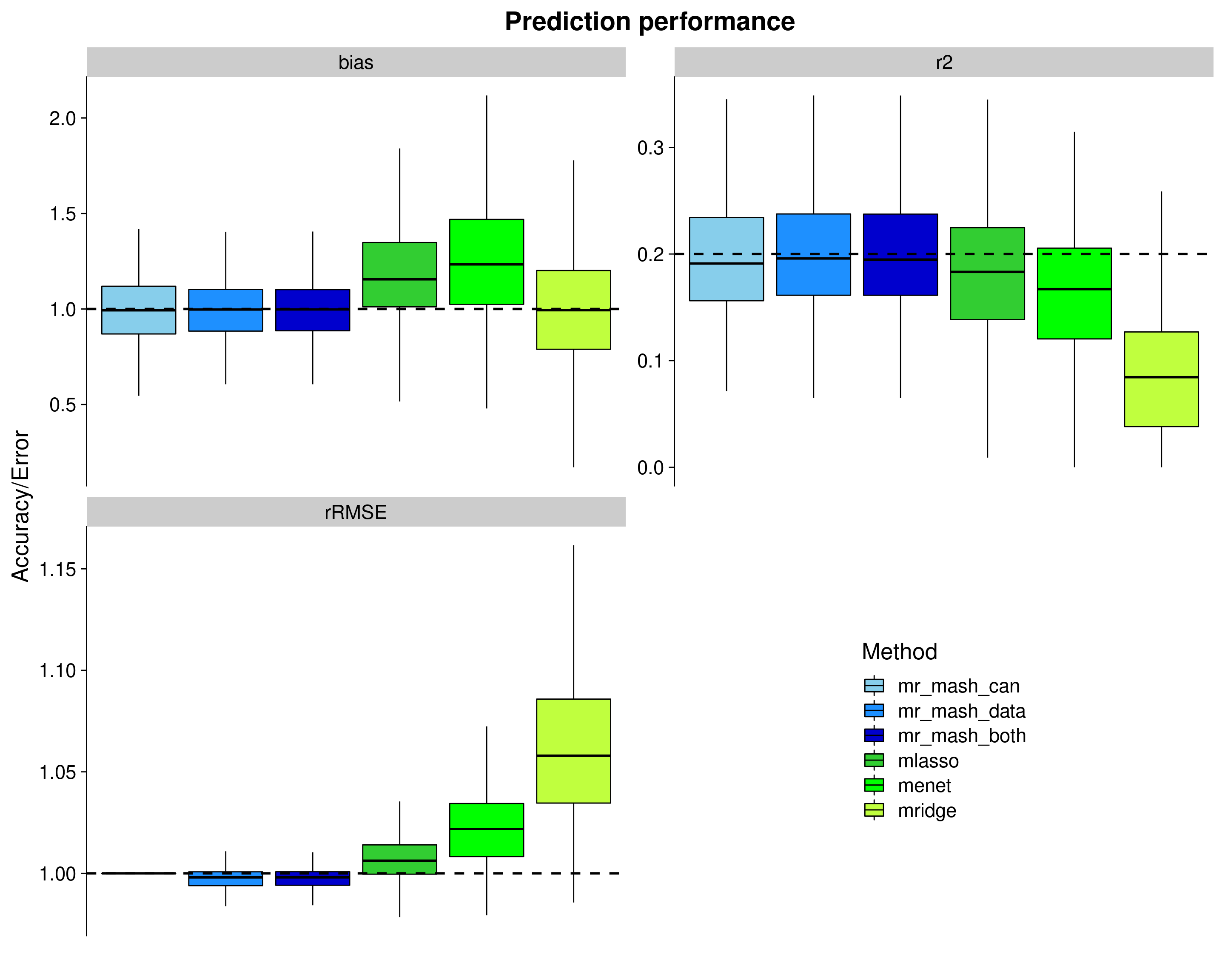
| Version | Author | Date |
|---|---|---|
| e2b7e5d | fmorgante | 2020-09-26 |
Here, we look at the elapsed time (\(log_{10}\) seconds) of each method. Note that the mr.mash run time does not include the run time of group-LASSO (but should be considered since we used it to initialize mr.mash).
dsc_plots_time <- dsc_plots[which(dsc_plots$response==1 & dsc_plots$score_metric=="r2"),
                          -which(colnames(dsc_plots) %in% c("score_metric", "score_value", "response"))]

p_time <- ggplot(dsc_plots_time, aes_string(x = "method_fac", y = "time", fill = "method_fac")) +
  geom_boxplot(color = "black", outlier.size = 1, width = 0.85) +
  scale_fill_manual(values = colors) +
  scale_y_continuous(trans="log10", breaks = trans_breaks("log10", function(x) 10^x),
                      labels = trans_format("log10", math_format(10^.x))) +
  labs(x = "", y = "Elapsed time (seconds) in log10 scale",title = "Run time", fill="Method") +
  theme_cowplot(font_size = 20) +
  theme(axis.line.x = element_blank(), axis.text.x = element_blank(), axis.ticks.x = element_blank(),
        plot.title = element_text(hjust = 0.5))

print(p_time)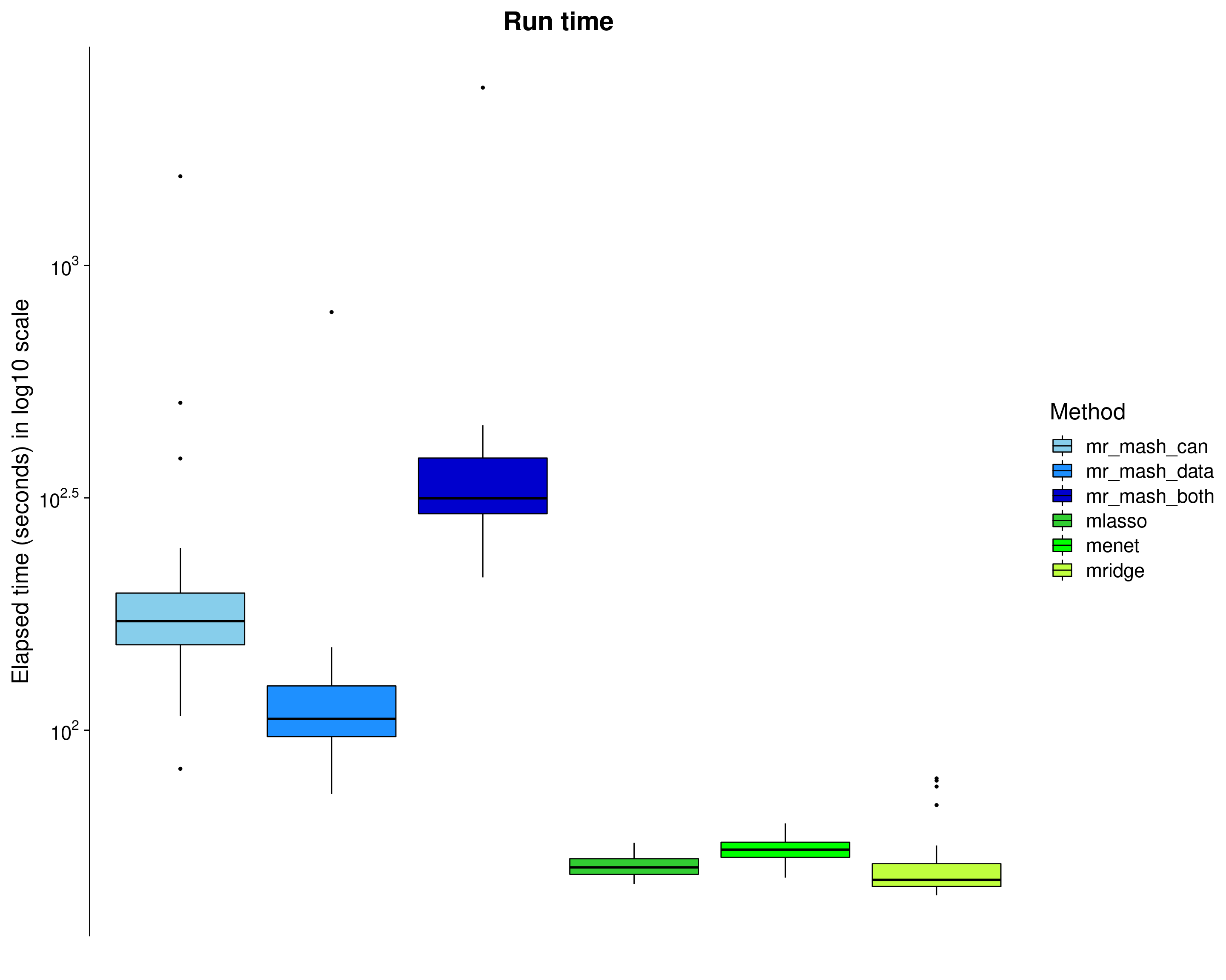
| Version | Author | Date |
|---|---|---|
| e2b7e5d | fmorgante | 2020-09-26 |
Highly correlated predictors
Simulation set up
###Load the dsc results
dsc_out <- dscquery("output/mvreg_all_genes_prior_highcorrX_indepV_sharedB_2blocksr10",
                    c("simulate.n", "simulate.p", "simulate.p_causal", "simulate.r",
                      "simulate.w","simulate.r_causal", "simulate.pve", "simulate.B_cor",
                      "simulate.B_scale", "simulate.X_cor", "simulate.X_scale",
                      "simulate.V_cor", "simulate", "fit", "score", "score.err", "fit.time"),
                    groups="fit: mr_mash_em_can, mr_mash_em_data, mr_mash_em_dataAndcan, mlasso, mridge, menet",
                    verbose=FALSE)

###Obtain simulation parameters
prop_testset <- 0.2
n <- unique(dsc_out$simulate.n)
p <- unique(dsc_out$simulate.p)
p_causal <- unique(dsc_out$simulate.p_causal)
r <- unique(dsc_out$simulate.r)
r_causal <- eval(parse(text=unique(dsc_out$simulate.r_causal)))
pve <- unique(dsc_out$simulate.pve)
w <- eval(parse(text=unique(dsc_out$simulate.w)))
B_cor <- eval(parse(text=unique(dsc_out$simulate.B_cor)))
B_scale <- eval(parse(text=unique(dsc_out$simulate.B_scale)))
X_cor <- unique(dsc_out$simulate.X_cor)
X_scale <- unique(dsc_out$simulate.X_scale)
V_cor <- unique(dsc_out$simulate.V_cor)

###Remove list elements that are not useful anymore
dsc_out$simulate.r_causal <- NULL
dsc_out$simulate.w <- NULL
dsc_out$simulate.B_cor <- NULL
dsc_out$simulate.B_scale <- NULL
dsc_out$simulate.X_cor <- NULL
dsc_out$simulate.X_scale <- NULL
dsc_out$simulate.V_cor <- NULL
This simulation is exactly as above, except that variables, X, were drawn from MVN(0, Gamma), where Gamma is such that it achieves a correlation between variables of 0.8 and a scale of 1.
mr.mash vs other methods
The fitting and prediction scheme and methods are as described above. Let’s look at \(r^2\), bias and rRMSE.
###Convert from list to data.frame for plotting
dsc_plots <- convert_dsc_to_dataframe(dsc_out)

###Compute rmse score (relative to mr_mash_consec_em) and add it to the data
rrmse_dat <- compute_rrmse(dsc_plots)
dsc_plots <- rbind(dsc_plots, rrmse_dat)

###Remove mse from scores and keep only methods wanted
dsc_plots <- dsc_plots[which(dsc_plots$score_metric!="scaled_mse" ), ]

###Create factor version of method
dsc_plots$method_fac <- factor(dsc_plots$method, levels=c("mr_mash_em_can", "mr_mash_em_data",
                                                          "mr_mash_em_dataAndcan", "mlasso", "menet", "mridge"),
                                                labels=c("mr_mash_can", "mr_mash_data", "mr_mash_both",
                                                         "mlasso", "menet", "mridge"))

###Build data.frame with best accuracy achievable
hlines <- data.frame(score_metric=c("r2", "bias", "rrmse"), max_val=c(unique(dsc_plots$pve), 1, 1))

###Create plots
p <- ggplot(dsc_plots, aes_string(x = "method_fac", y = "score_value", fill = "method_fac")) +
    geom_boxplot(color = "black", outlier.size = 1, width = 0.85) +
    facet_wrap(vars(score_metric), scales="free_y", ncol=2, labeller=labeller(score_metric=facet_labels)) +
    scale_fill_manual(values = colors) +
    labs(x = "", y = "Accuracy/Error", title = "Prediction performance", fill="Method") +
    geom_hline(data=hlines, aes(yintercept = max_val), linetype="dashed", size=1) +
    theme_cowplot(font_size = 20) +
    theme(axis.line.x = element_blank(), axis.text.x = element_blank(), axis.ticks.x = element_blank(),
          plot.title = element_text(hjust = 0.5))

shift_legend(p)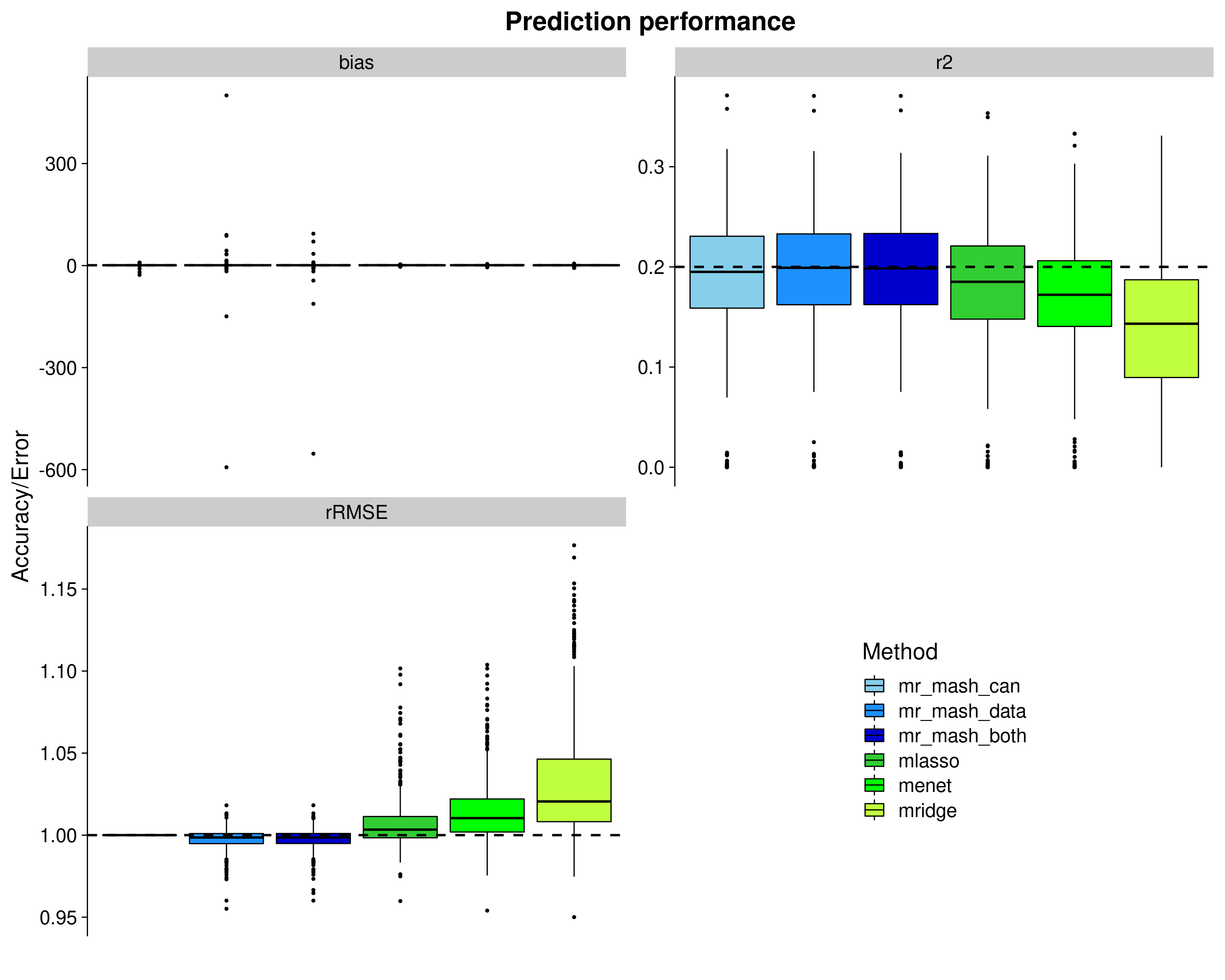
| Version | Author | Date |
|---|---|---|
| e2b7e5d | fmorgante | 2020-09-26 |
Let’s now remove outliers from the plots to make things a little clearer.
###Create plots
p_nooutliers <- ggplot(dsc_plots, aes_string(x = "method_fac", y = "score_value", fill = "method_fac")) +
    Ipaper::geom_boxplot2(color = "black", width = 0.85, width.errorbar = 0) +
    facet_wrap(vars(score_metric), scales="free_y", ncol=2, labeller=labeller(score_metric=facet_labels)) +
    scale_fill_manual(values = colors) +
    labs(x = "", y = "Accuracy/Error", title = "Prediction performance", fill="Method") +
    geom_hline(data=hlines, aes(yintercept = max_val), linetype="dashed", size=1) +
    theme_cowplot(font_size = 20) +
    theme(axis.line.x = element_blank(), axis.text.x = element_blank(), axis.ticks.x = element_blank(),
          plot.title = element_text(hjust = 0.5))

shift_legend(p_nooutliers)
| Version | Author | Date |
|---|---|---|
| e2b7e5d | fmorgante | 2020-09-26 |
Here, we look at the elapsed time (\(log_{10}\) seconds) of each method. Note that the mr.mash run time does not include the run time of group-LASSO (but should be considered since we used it to initialize mr.mash).
dsc_plots_time <- dsc_plots[which(dsc_plots$response==1 & dsc_plots$score_metric=="r2"),
                          -which(colnames(dsc_plots) %in% c("score_metric", "score_value", "response"))]

p_time <- ggplot(dsc_plots_time, aes_string(x = "method_fac", y = "time", fill = "method_fac")) +
  geom_boxplot(color = "black", outlier.size = 1, width = 0.85) +
  scale_fill_manual(values = colors) +
  scale_y_continuous(trans="log10", breaks = trans_breaks("log10", function(x) 10^x),
                      labels = trans_format("log10", math_format(10^.x))) +
  labs(x = "", y = "Elapsed time (seconds) in log10 scale",title = "Run time", fill="Method") +
  theme_cowplot(font_size = 20) +
  theme(axis.line.x = element_blank(), axis.text.x = element_blank(), axis.ticks.x = element_blank(),
        plot.title = element_text(hjust = 0.5))

print(p_time)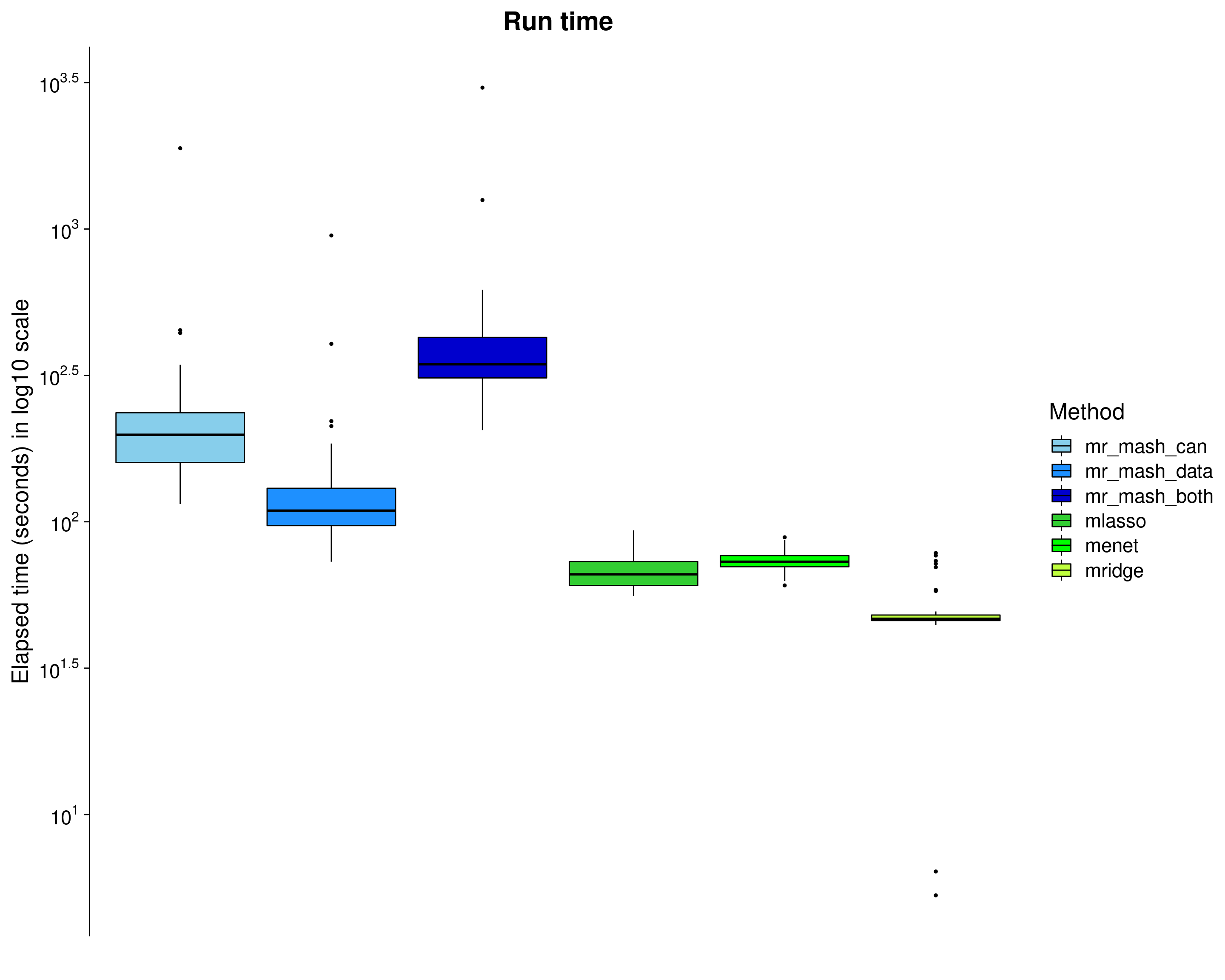
| Version | Author | Date |
|---|---|---|
| e2b7e5d | fmorgante | 2020-09-26 |
In summary, mr.mash with the data-driven covariance matrices does very well and runs pretty fast. Using only the canonical covariance matrices is not as effective (as expected) in this case, but it’s still good. Using both types of covariance matrices does not add anything in terms of performance to using only the data-driven matrices. However, it makes the method much slower to run.
sessionInfo()R version 3.5.1 (2018-07-02)
Platform: x86_64-pc-linux-gnu (64-bit)
Running under: Scientific Linux 7.4 (Nitrogen)
Matrix products: default
BLAS/LAPACK: /software/openblas-0.2.19-el7-x86_64/lib/libopenblas_haswellp-r0.2.19.so
locale:
[1] LC_CTYPE=en_US.UTF-8 LC_NUMERIC=C
[3] LC_TIME=en_US.UTF-8 LC_COLLATE=en_US.UTF-8
[5] LC_MONETARY=en_US.UTF-8 LC_MESSAGES=en_US.UTF-8
[7] LC_PAPER=en_US.UTF-8 LC_NAME=C
[9] LC_ADDRESS=C LC_TELEPHONE=C
[11] LC_MEASUREMENT=en_US.UTF-8 LC_IDENTIFICATION=C
attached base packages:
[1] stats graphics grDevices utils datasets methods base
other attached packages:
[1] devtools_2.1.0 usethis_1.5.1 magrittr_1.5 lemon_0.4.3
[5] gtable_0.3.0 scales_1.1.1 cowplot_1.0.0 ggplot2_3.3.2
[9] dscrutils_0.4.2
loaded via a namespace (and not attached):
[1] pkgload_1.1.0 jsonlite_1.6 foreach_1.4.4
[4] Ipaper_0.1.5 assertthat_0.2.1 sp_1.3-1
[7] cellranger_1.1.0 yaml_2.2.1 remotes_2.1.0
[10] progress_1.2.2 sessioninfo_1.1.1 pillar_1.4.4
[13] backports_1.1.8 lattice_0.20-38 glue_1.4.1
[16] digest_0.6.25 RColorBrewer_1.1-2 promises_1.0.1
[19] colorspace_1.4-1 htmltools_0.3.6 httpuv_1.4.5
[22] plyr_1.8.6 clipr_0.4.1 pkgconfig_2.0.3
[25] purrr_0.3.3 processx_3.4.2 whisker_0.3-2
[28] openxlsx_4.1.0 later_0.7.5 git2r_0.26.1
[31] tibble_3.0.1 farver_2.0.3 ellipsis_0.3.1
[34] withr_2.2.0 repr_0.17 cli_2.0.2
[37] crayon_1.3.4 readxl_1.1.0 memoise_1.1.0
[40] evaluate_0.14 ps_1.3.3 fs_1.3.1
[43] fansi_0.4.1 doParallel_1.0.14 xml2_1.2.0
[46] pkgbuild_1.0.8 tools_3.5.1 data.table_1.12.8
[49] prettyunits_1.1.1 hms_0.5.3 matrixStats_0.56.0
[52] lifecycle_0.2.0 stringr_1.4.0 munsell_0.5.0
[55] zip_1.0.0 callr_3.4.3 compiler_3.5.1
[58] rlang_0.4.6 grid_3.5.1 rstudioapi_0.11
[61] iterators_1.0.10 base64enc_0.1-3 labeling_0.3
[64] rmarkdown_1.10 boot_1.3-20 testthat_2.3.2
[67] codetools_0.2-15 reshape2_1.4.4 R6_2.4.1
[70] lubridate_1.7.4 gridExtra_2.3 knitr_1.20
[73] dplyr_0.8.0.1 workflowr_1.6.2 rprojroot_1.3-2
[76] desc_1.2.0 stringi_1.4.6 parallel_3.5.1
[79] IRdisplay_0.6.1 Rcpp_1.0.5 vctrs_0.3.1
[82] tidyselect_0.2.5