IMC Cell Segmentation using QuPath, ImageJ, and Mesmer
Givanna Putri
2025-11-25
Last updated: 2025-11-26
Checks: 7 0
Knit directory:
2025_cytoconnect_spatial_workshop/
This reproducible R Markdown analysis was created with workflowr (version 1.7.2). The Checks tab describes the reproducibility checks that were applied when the results were created. The Past versions tab lists the development history.
Great! Since the R Markdown file has been committed to the Git repository, you know the exact version of the code that produced these results.
Great job! The global environment was empty. Objects defined in the global environment can affect the analysis in your R Markdown file in unknown ways. For reproduciblity it’s best to always run the code in an empty environment.
The command set.seed(20251002) was run prior to running
the code in the R Markdown file. Setting a seed ensures that any results
that rely on randomness, e.g. subsampling or permutations, are
reproducible.
Great job! Recording the operating system, R version, and package versions is critical for reproducibility.
Nice! There were no cached chunks for this analysis, so you can be confident that you successfully produced the results during this run.
Great job! Using relative paths to the files within your workflowr project makes it easier to run your code on other machines.
Great! You are using Git for version control. Tracking code development and connecting the code version to the results is critical for reproducibility.
The results in this page were generated with repository version a88eee1. See the Past versions tab to see a history of the changes made to the R Markdown and HTML files.
Note that you need to be careful to ensure that all relevant files for
the analysis have been committed to Git prior to generating the results
(you can use wflow_publish or
wflow_git_commit). workflowr only checks the R Markdown
file, but you know if there are other scripts or data files that it
depends on. Below is the status of the Git repository when the results
were generated:
Ignored files:
    Ignored:    .DS_Store
    Ignored:    data/.DS_Store
    Ignored:    data/imc/
    Ignored:    data/visium/

Unstaged changes:
    Modified:   analysis/imc_02.Rmd
Note that any generated files, e.g. HTML, png, CSS, etc., are not included in this status report because it is ok for generated content to have uncommitted changes.
These are the previous versions of the repository in which changes were
made to the R Markdown (analysis/imc_01.Rmd) and HTML
(docs/imc_01.html) files. If you’ve configured a remote Git
repository (see ?wflow_git_remote), click on the hyperlinks
in the table below to view the files as they were in that past version.
| File | Version | Author | Date | Message |
|---|---|---|---|---|
| Rmd | a88eee1 | Givanna Putri | 2025-11-26 | wflow_publish("analysis/imc_01.Rmd") |
Introduction
In this part of IMC analysis, we will focus on cell segmentation using popular tools QuPath and ImageJ with the Mesmer plugin. Accurate cell segmentation is crucial for downstream analysis, as it allows us to quantify marker expressions at the single-cell level.
To be able to follow this tutorial, please ensure you have the following software installed:
- Qupath 0.6.0: https://qupath.readthedocs.io/en/stable/index.html
- ImageJ: https://imagej.net/ij/
- DeepCell ImageJ plugin: https://github.com/vanvalenlab/kiosk-imageJ-plugin
For this tutorial, we will be using the 35-marker IMC panel on FFPE
human intestines. The paper describing the data:
https://doi.org/10.1002/cyto.a.24847. The panel is designed
to delineate various immune cell subsets and HIV RNA.
The data can be downloaded either from the Google drive link in the setup page or from Zenodo.
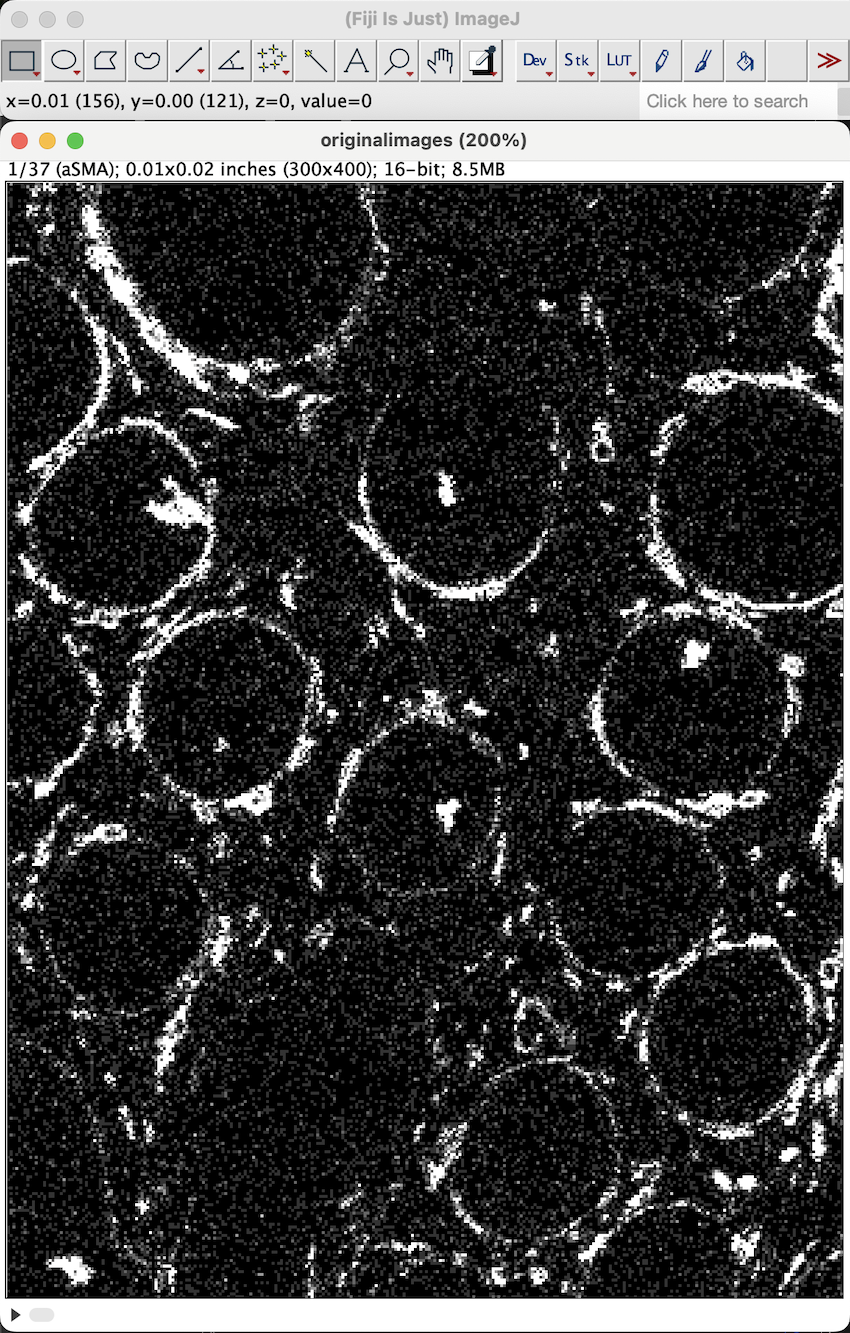
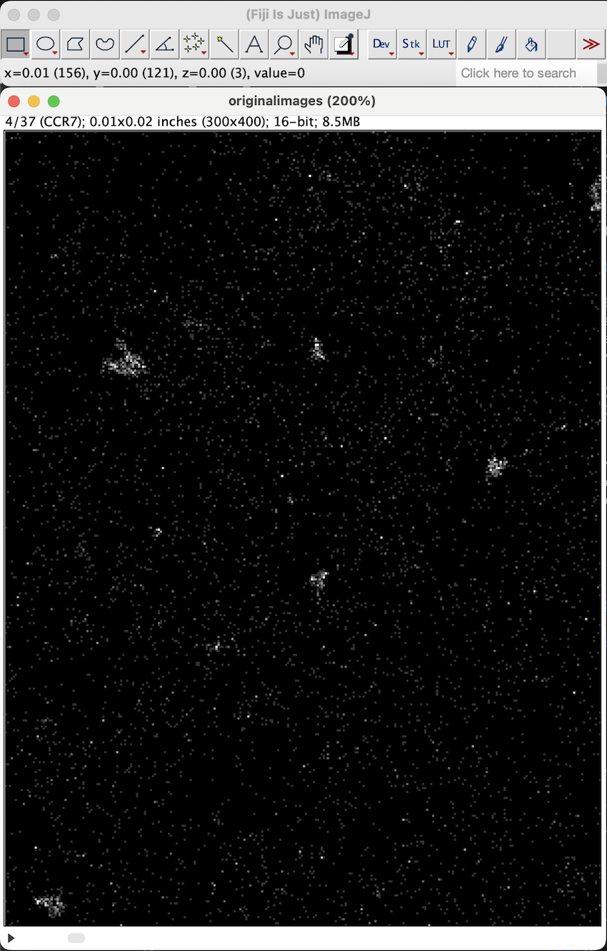
Preparing Tif files for segmentation
The dataset is provided as single channel tiff files for each marker. Hence when you download the data, you will get a folder structure like this:
imc
└──tif_files
   └── originalimages
        ├── aSMA.tif
        ├── Axl.tif
        ├── CCR6.tif
        └── ...
As previously mentioned in the introduction, we generally use membrane/cytoplasm and nuclei markers for segmentation. For this dataset, we will use 3 membrane markers: CD45, E-cadherin, and NaKATPase. For nuclei, we will use DNA1.
Merging membrane markers using ImageJ
We will first prepare the merged membrane marker using ImageJ.
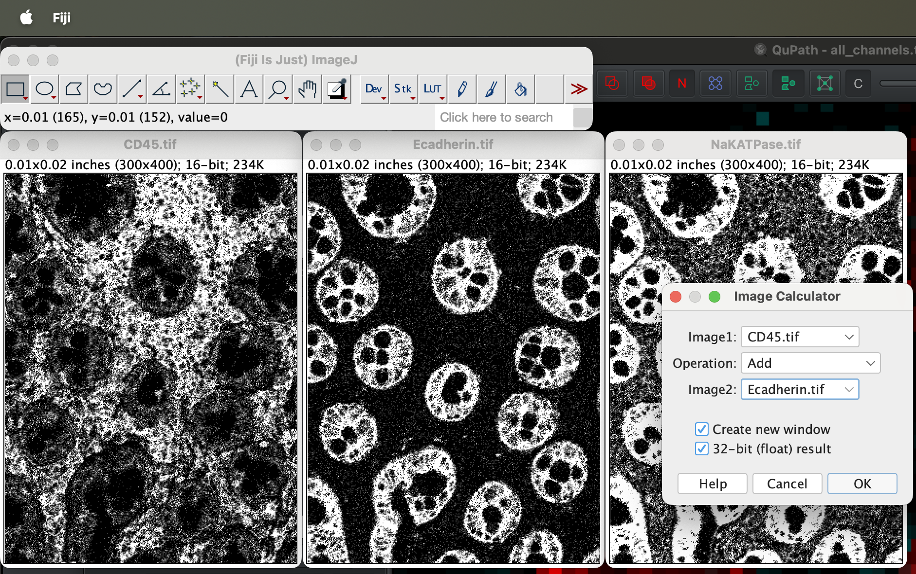
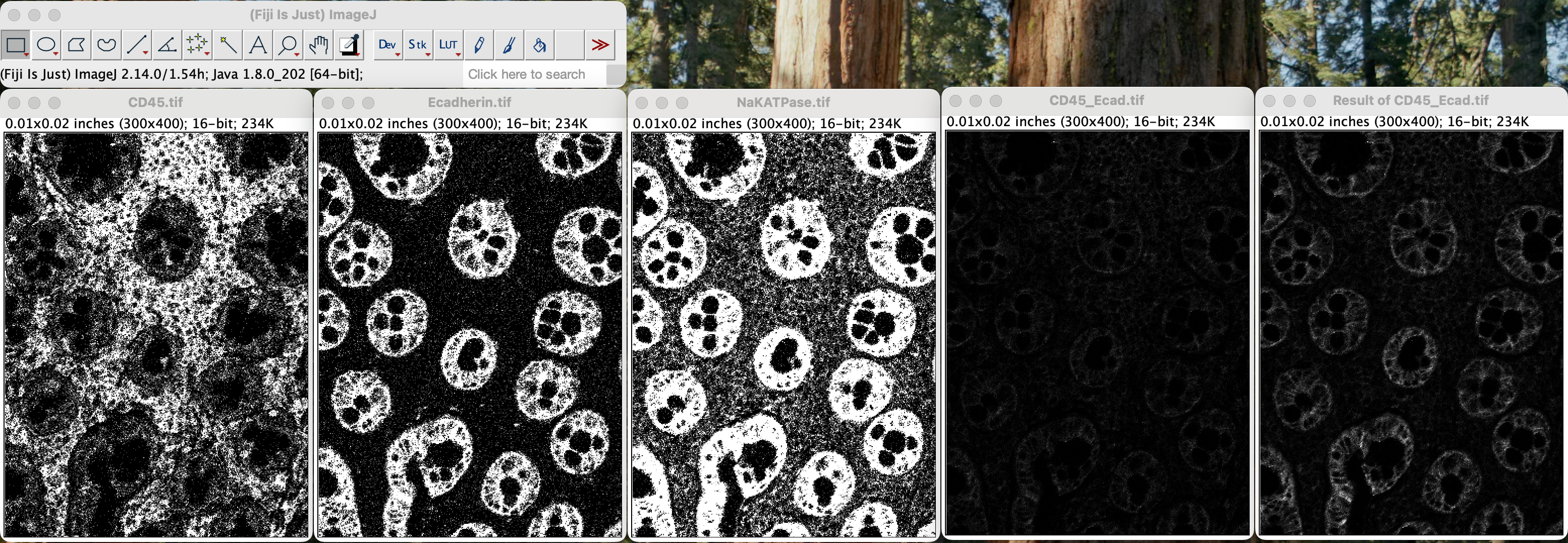
First, open CD45.tif, Ecadherin.tif,
NaKATPase.tif in ImageJ. One window per image.
Go to Process → Image Calculator to add the channels in order.
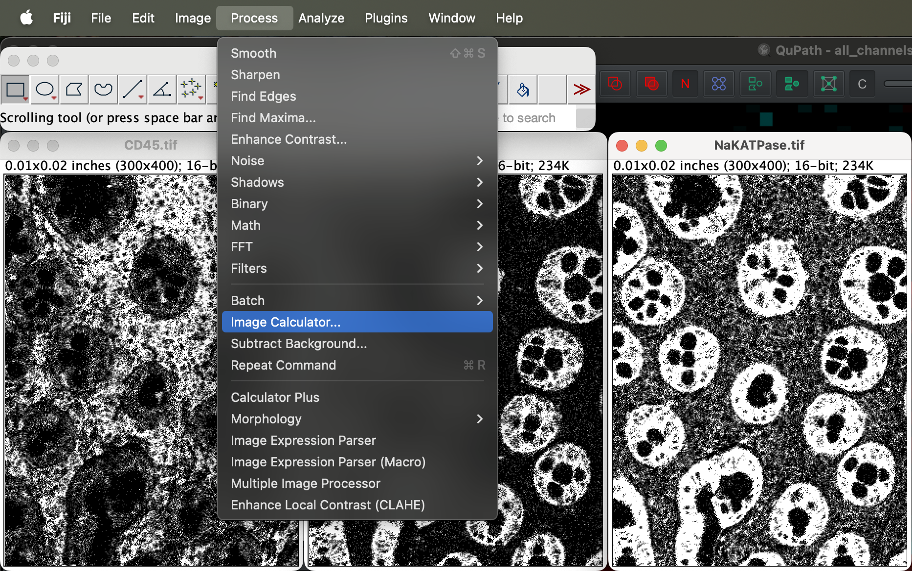
Select image 1 as the CD45 and Ecadherin as image 2. You will then get a new window called Result of CD45 as a result.
Save it as CD45_Ecadherin.tif somewhere in your
computer.
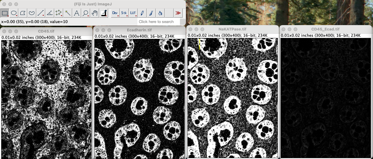
Repeat the process but select CD45_Ecadherin.tifas image
1 and NAKatPase as image 2.
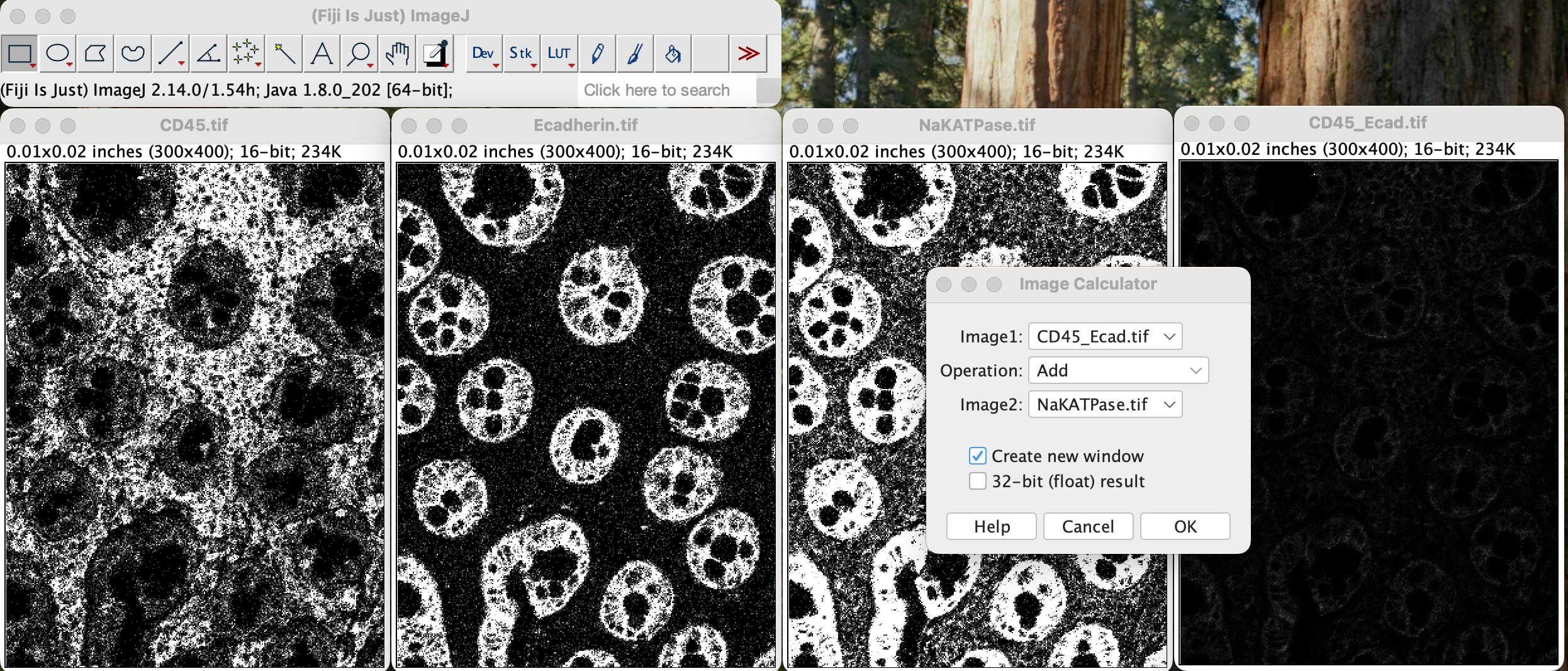
You will get a new window called Result of CD45_Ecad.tif
window.
Add a small amount of gaussian filter to blur them out so they don’t look like 3 separate channels. Go to Process → Filters → Gaussian Blur with small sigma (1–2 px).
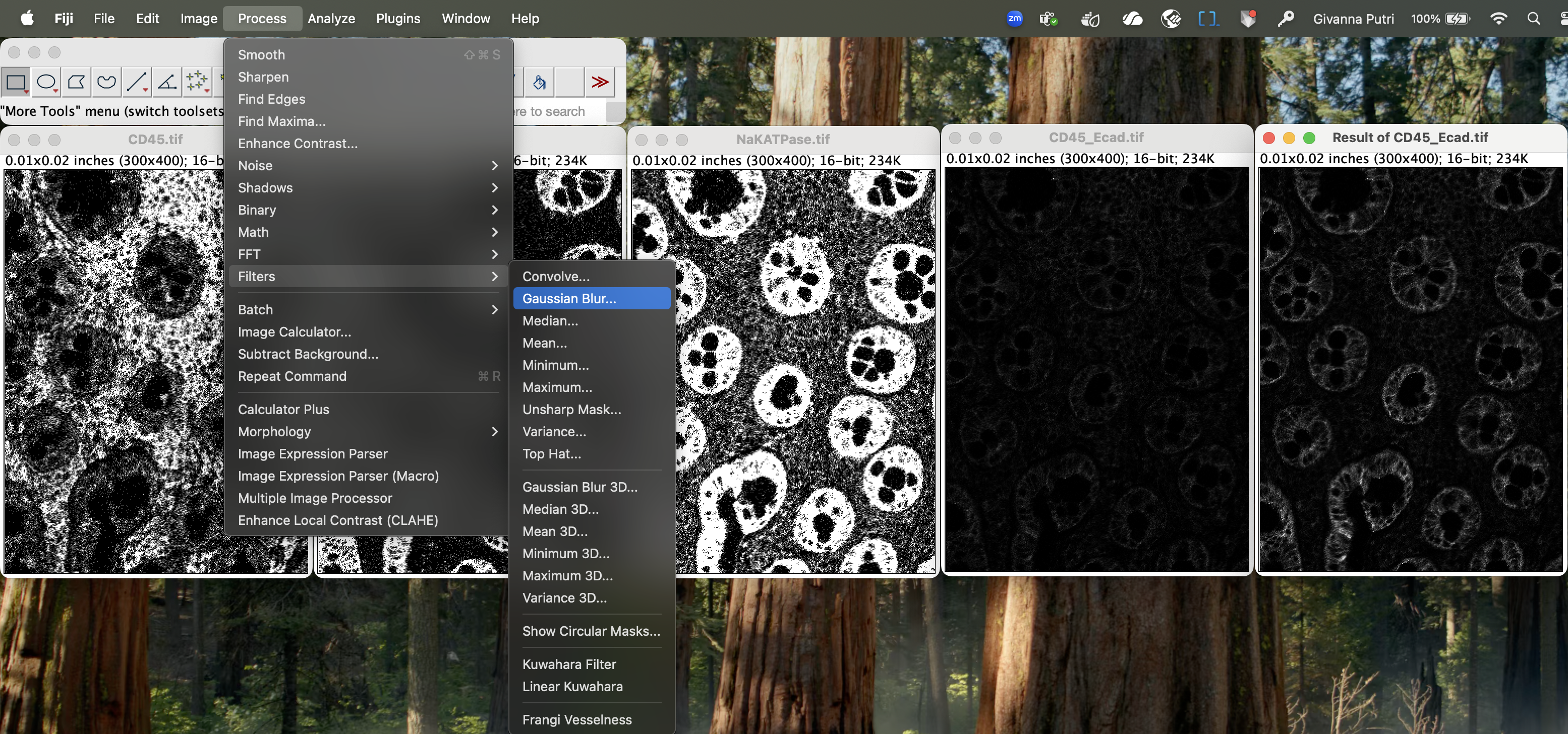
You can tick the “Preview” checkbox to see what the resulting image will look like after applying certain sigma values. The lower the sigma value, the less blurring there will be.
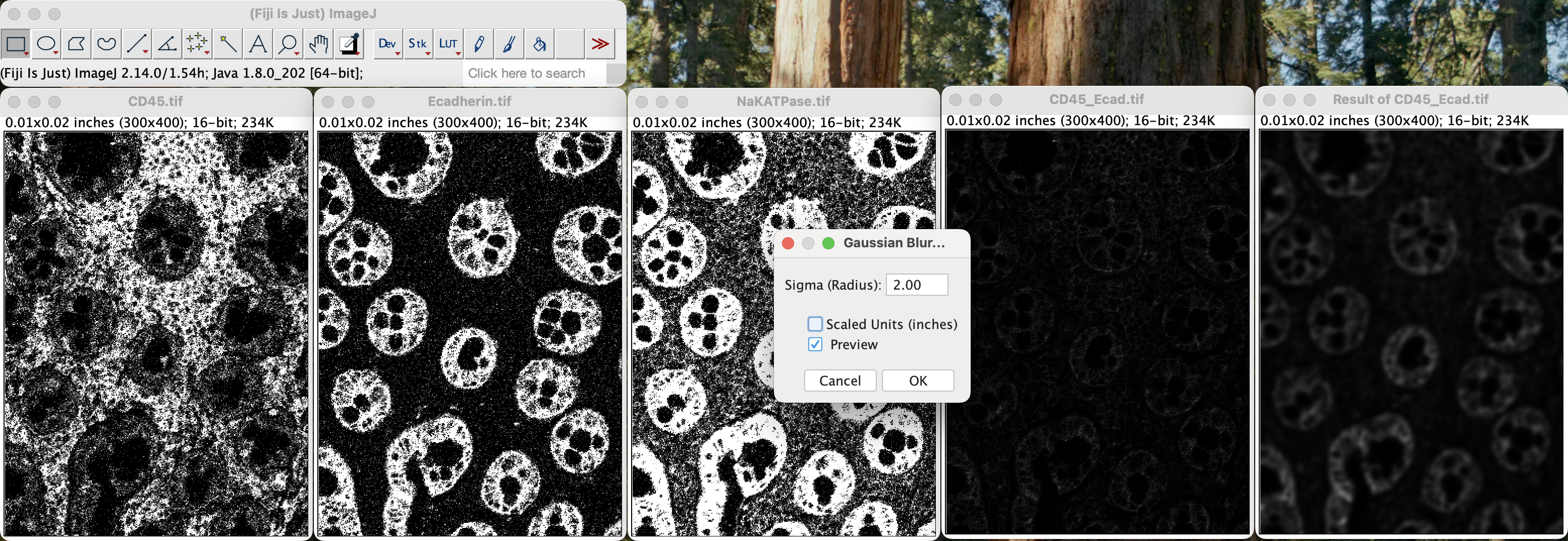
Then save the image as membrane_channel_combined.tif
Creating stack tiff files
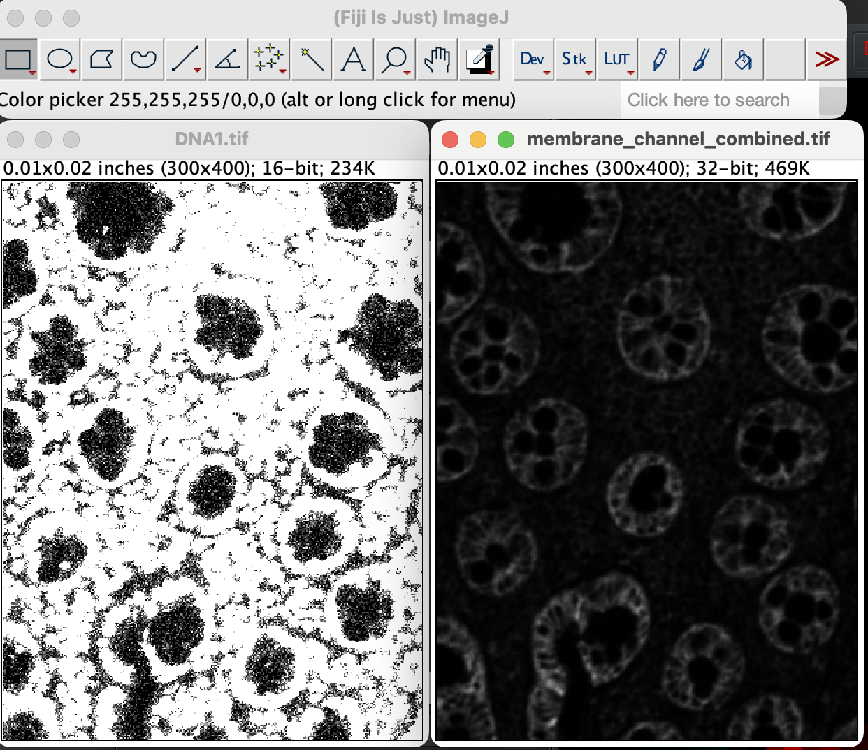
Before sending the tif file to mesmer for segmentation, we need to first create a stack tif file containing the DNA1 tif file and the merged membrane channel tif file we created in the previous section.
First open the DNA1 image and the merged membrane channel tif file in that order. The order is important because Mesmer require the nuclei stain to be the very 1st layer, followed by the membrane layer. Opening the DNA1 first will allow us to specify the DNA channel as as the very 1st layer, followed by the membrane channel.
Next, go to Image → stacks → Image to Stack.
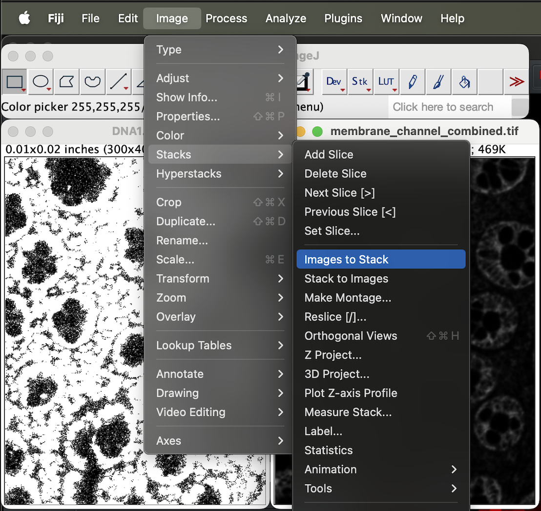
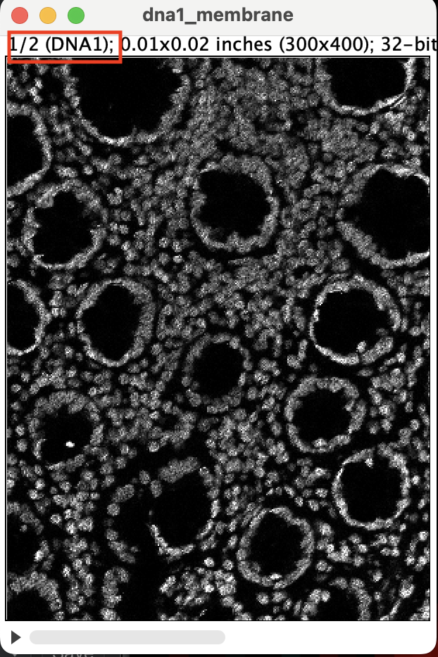
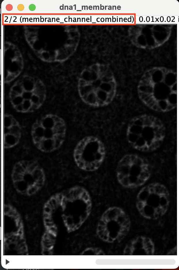
You should get a stacked image. Make sure stack 1 of 2 is DNA1 and
stack 2 is the membrane channel. You can flick through the stack using
the left and right arrow key. If the stacks are ordered correctly, you
should see 1/2 next to the DNA1 and 2/2 next to
membrane_channel_combined.
Save the image, use any file name.
Segmentation using Mesmer
Now we are ready to send our file to DeepCell server to be segmented.
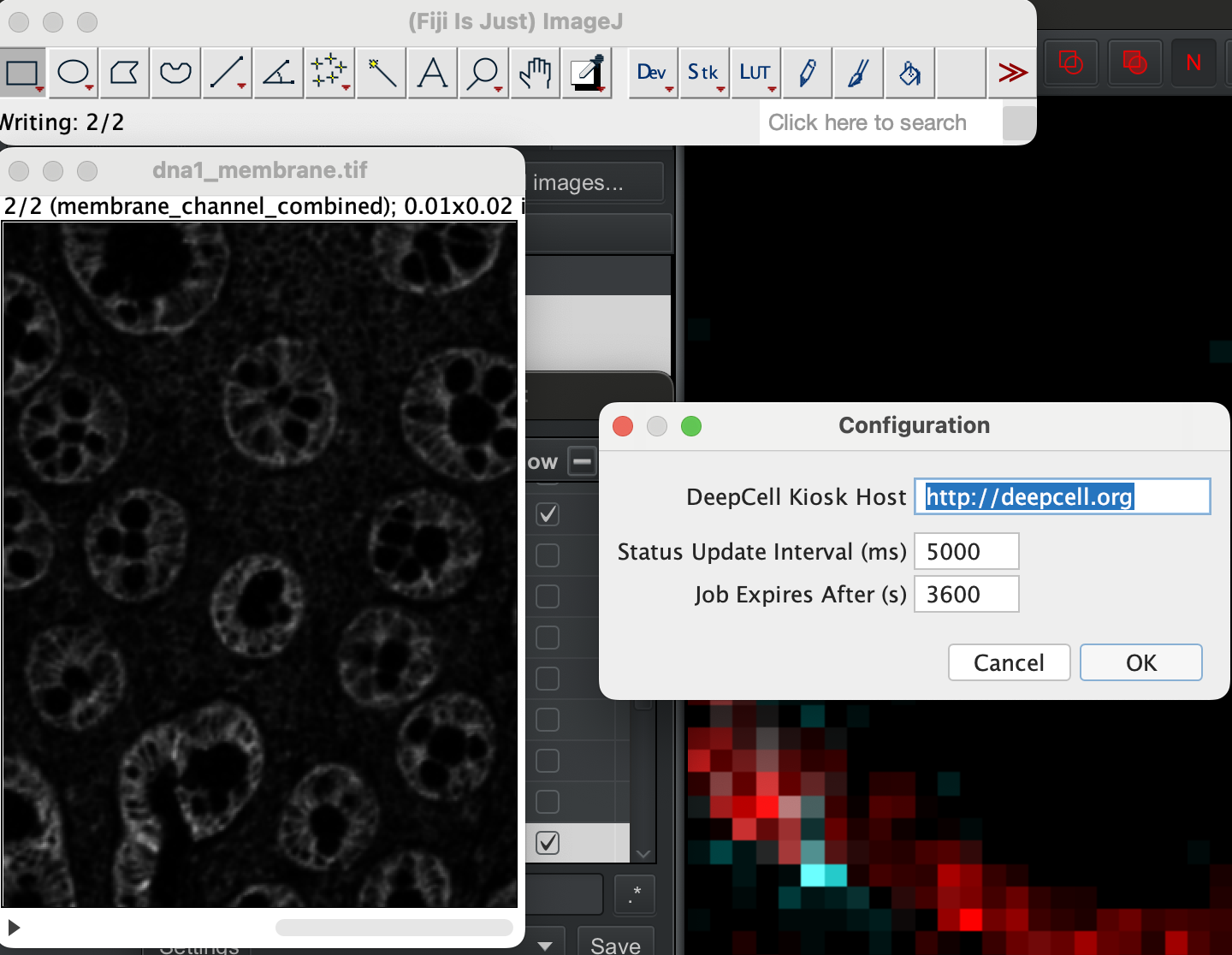
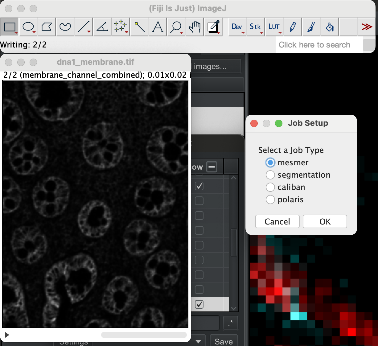
With the stack image open, select the image, then go to Plugin → DeepCell Kiosk → Submit Active Image.
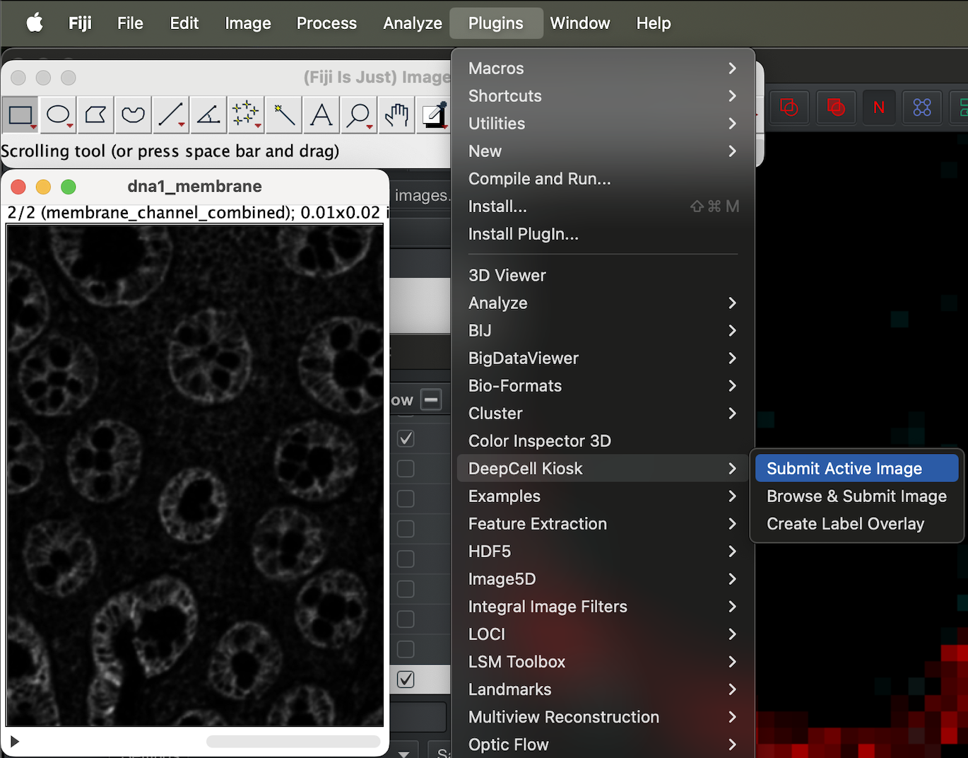
You can leave the config as it is and just click ok.
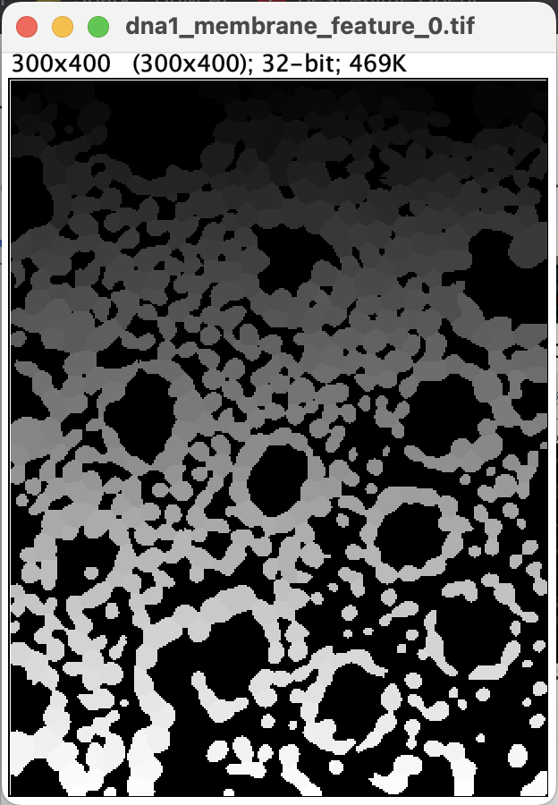
On the menu bar you should see a progress bar showing the status.

When it is done you should get the segmentation mask.
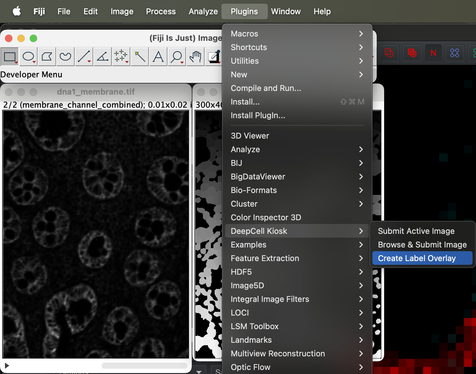
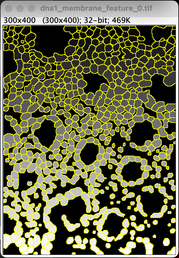
Before we can import the segmentation to Qupath for closer inspection, we have to first generate the label overlay. Go to Plugin → DeepCell Kiosk → Create label overlay.
Once it is done you will get the cell outlines like so.
You can then export it by going to Image → Overlay → To ROI manager.
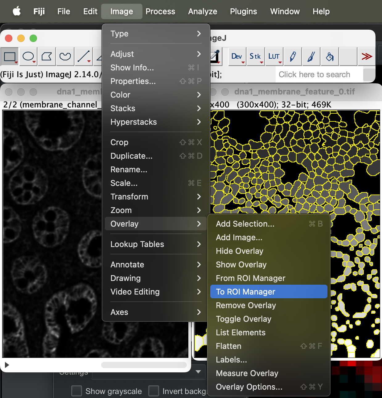
Select more at bottom right of the window then save.
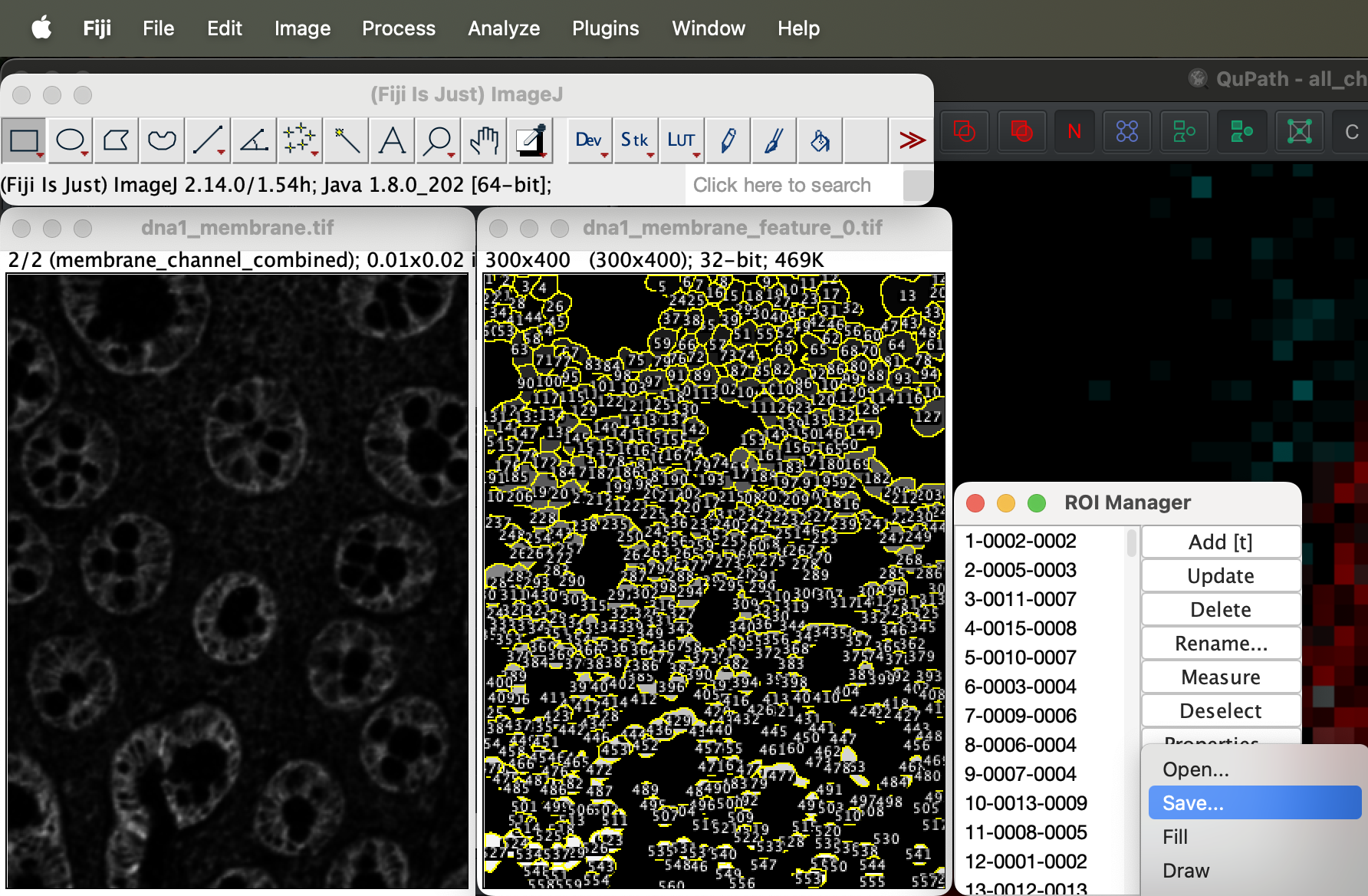
It should export the ROI as a zip file.
Visualising tissue using QuPath
Before we can view all the channels in QuPath, we need to first convert all the single channel tif files (1 channel = 1 tif file) into one stack image and save it.
Creating stack tif file
We can do this using ImageJ.
Go to File → Import → Image Sequence. Click browser to select the folder containing all the tif files and click ok.
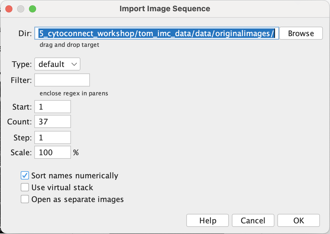
When done, you should have an image with 37 channels. You can switch between different channels using the left and right arrow keys. You can also zoom in and out of the image using the up and down arrow keys respectively.
We have to then convert it to hyperstack. Go to Image → Hyperstacks → Stack to Hyperstack.
Set the channels to how many markers you have (37 in this dataset) and slice to 1. Leave the order as it is as that’s how qupath likes it.
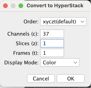
Then save as tiff file.
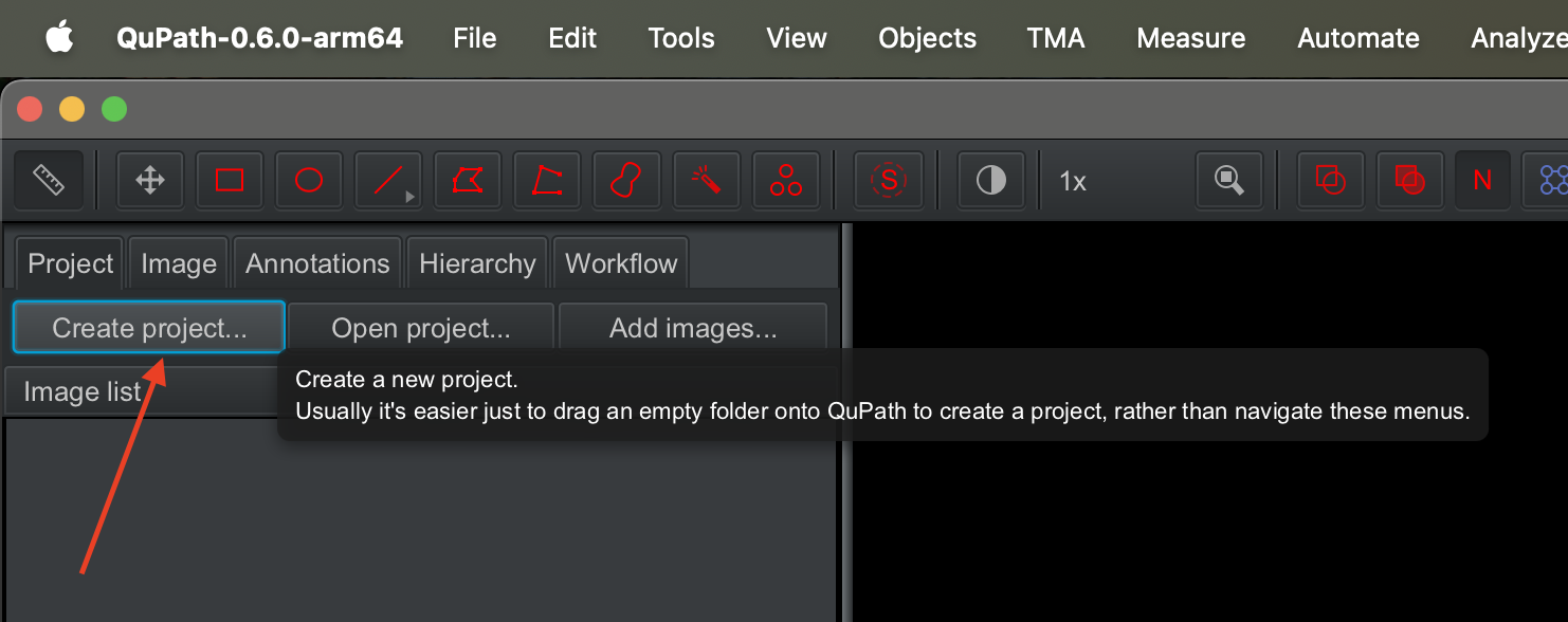
Interacting with the tif file using QuPath
Create a qupath project by clicking on the
create project... button on the right.
Pick where you want to store the files associated with the project.
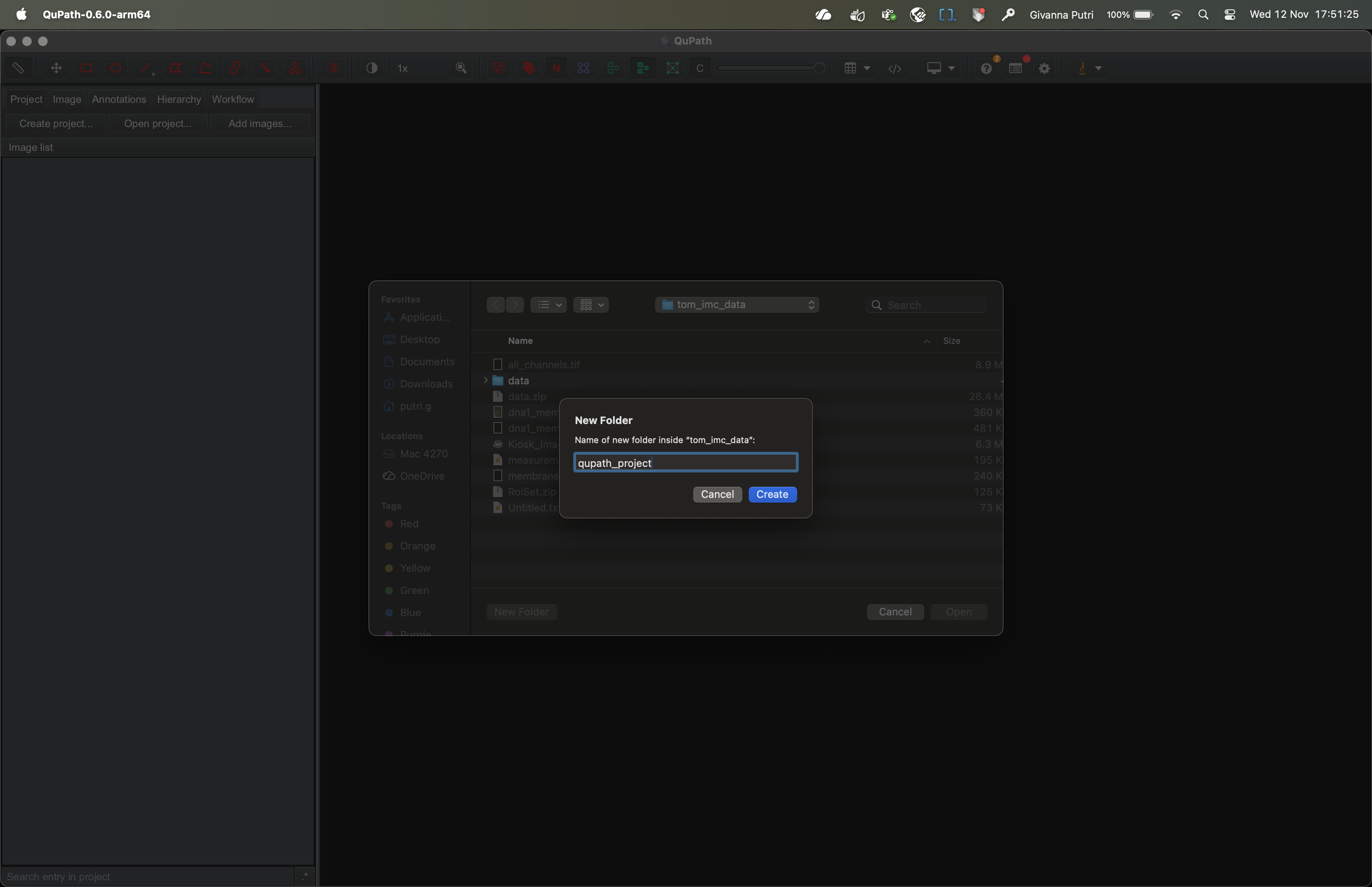
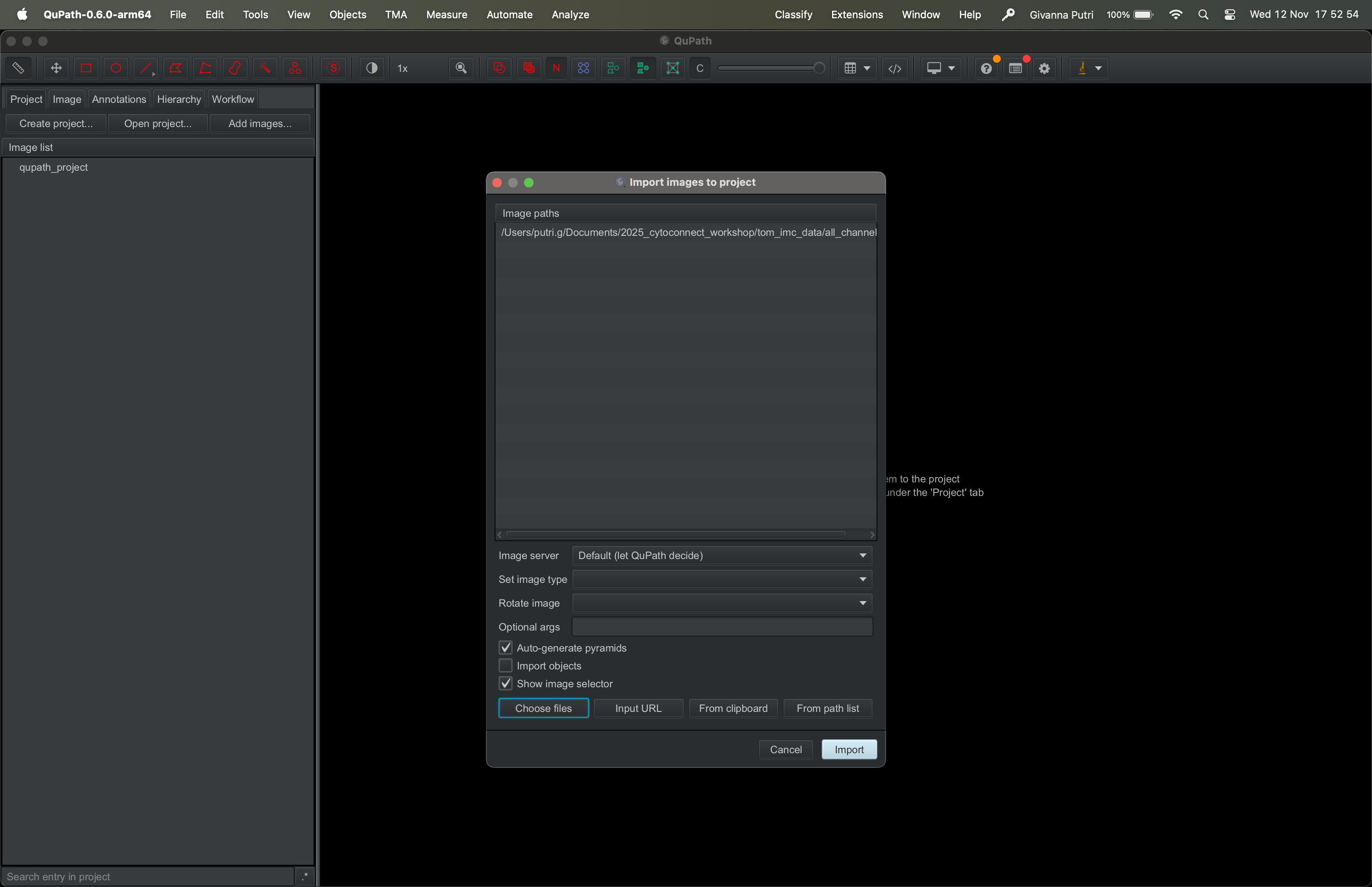
You will then be asked to add images to the QuPath project. Click
Choose files and select the directory where you store the
tif stack tif file we created in the previous section. Then click
import.
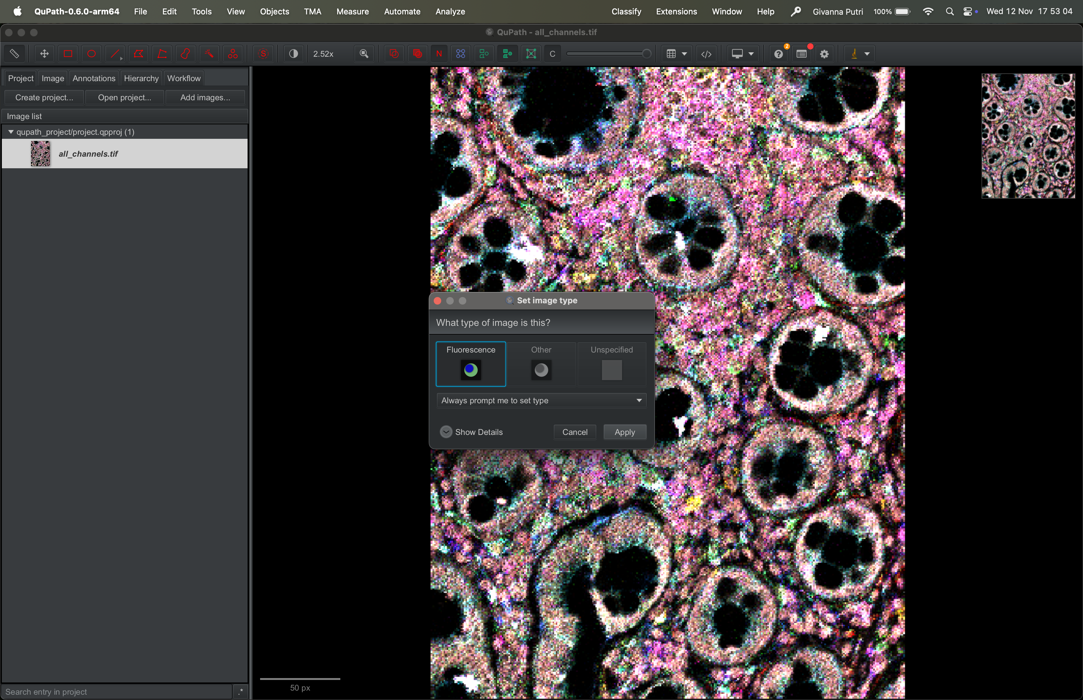
Qupath will ask you what type of image this is. Its guesses are generally pretty accurate.
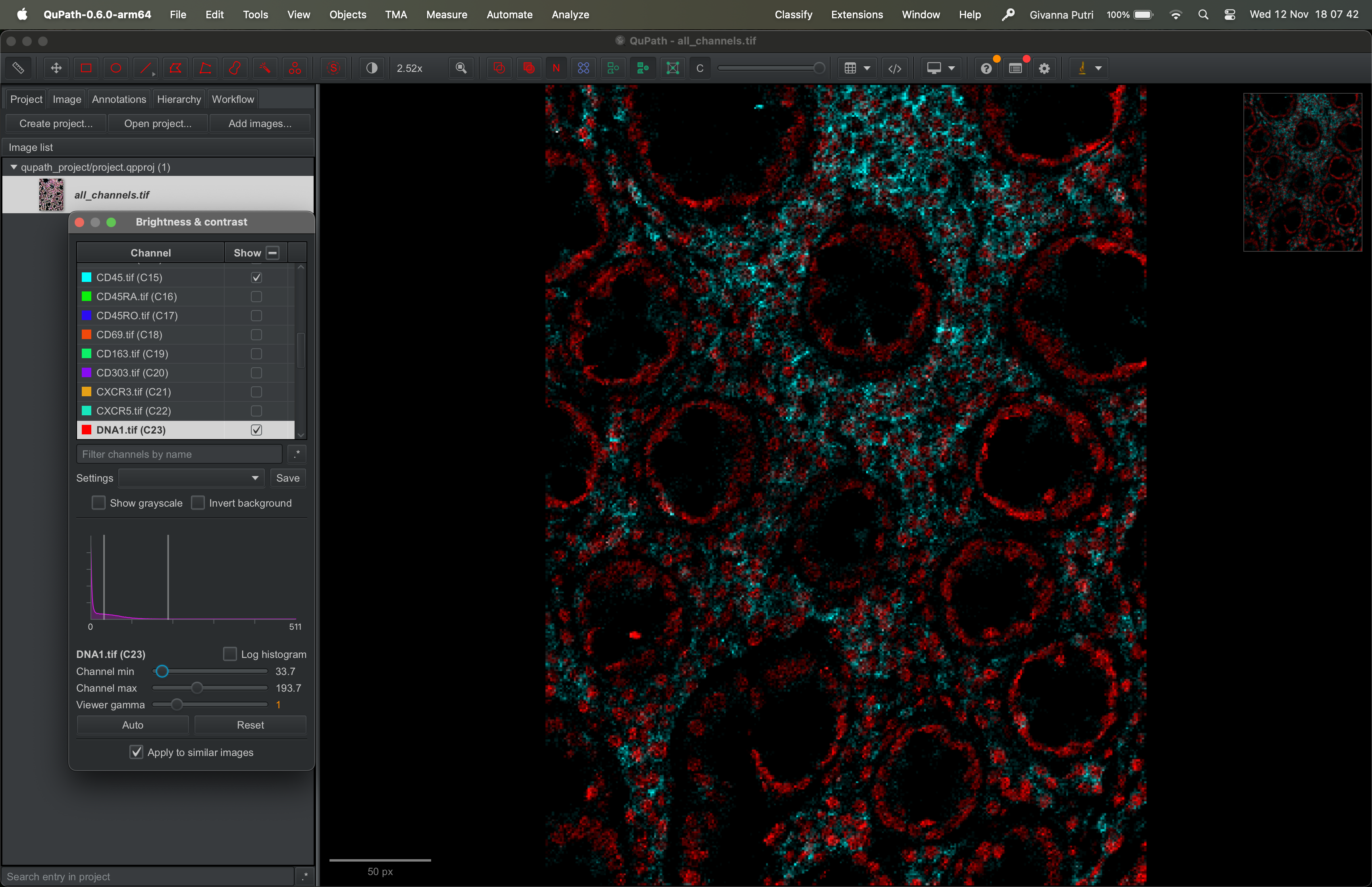
By default, it will show all the channels and there will be overlaps in colours.
To pick which channel to show, go to View → Brightness/Contrast. Untick all channels, then tick whichever you want to show. In example below, I picked DNA1 (red) and CD45 (turquoise).
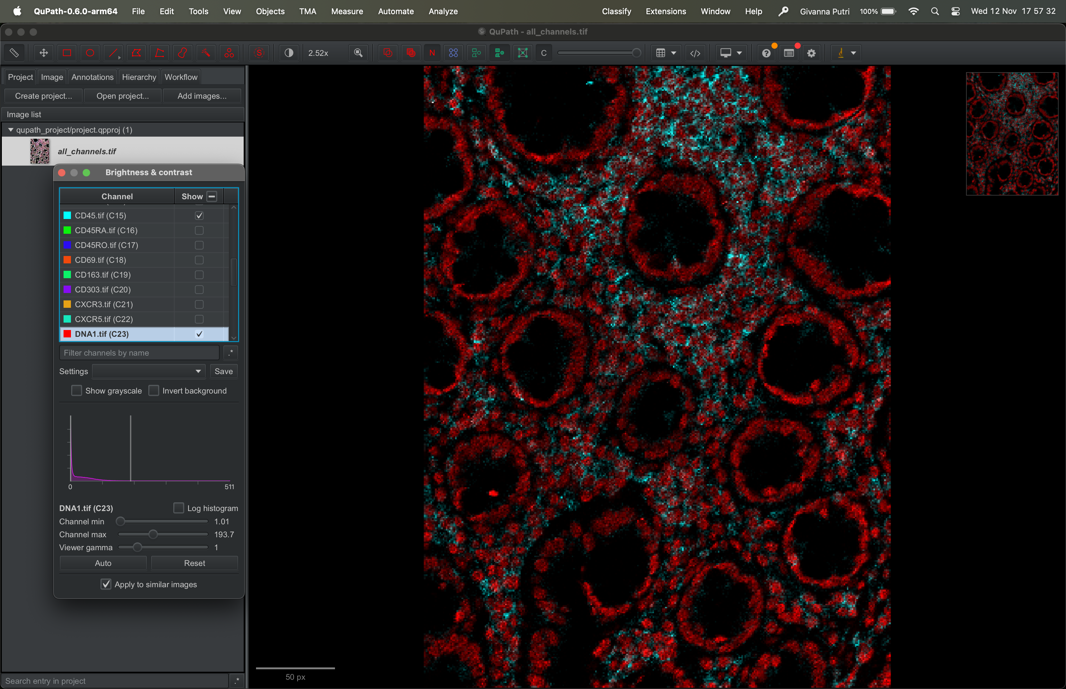
When you view a stack image (DNA1 and CD45 in the example above), each channel is shown with its own intensity range. The range is usually from the minimum pixel value to the maximum pixel value.
If a channel has very bright signal (like DNA1 in our example above), it can visually dominate the display. We can reduce its apparent brightness by changing how QuPath maps pixel intensities to display brightness.
You can either move the max slider to the right, which tells qupath any value larger than this threshold will be “whiter”. Or move the min slider to the right, which tells qupath to exaggerate the contrast.
This doesn’t change your data — it just changes how it’s visualized.
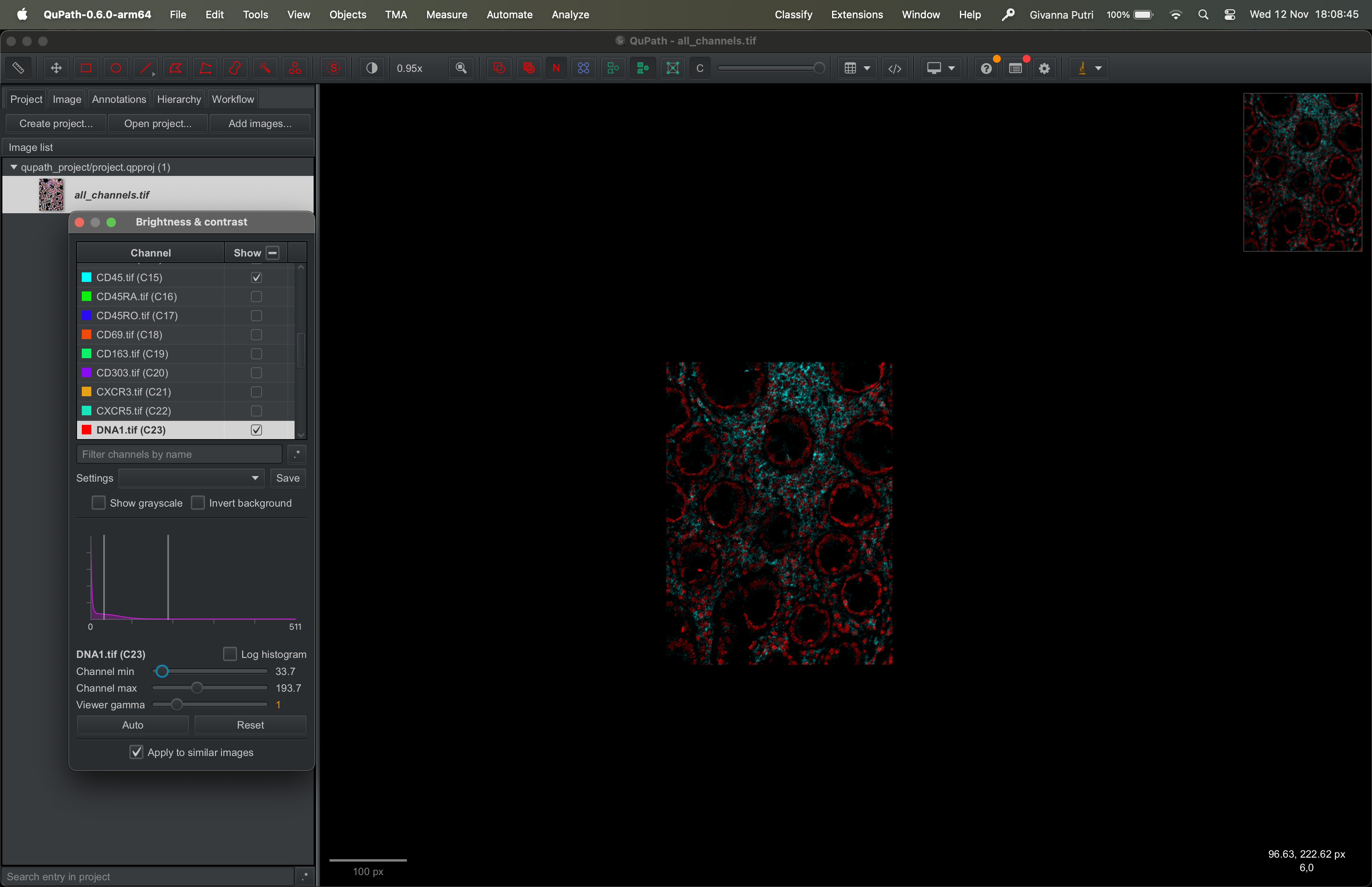
You can zoom in and out of the image by scrolling on the image up or down. The scale of the zoom is showed on the bottom left of the image.
Zoom out:
Zoom in:

Importing segmentation masks
Go to Extensions → ImageJ → Import ImageJ ROIs.
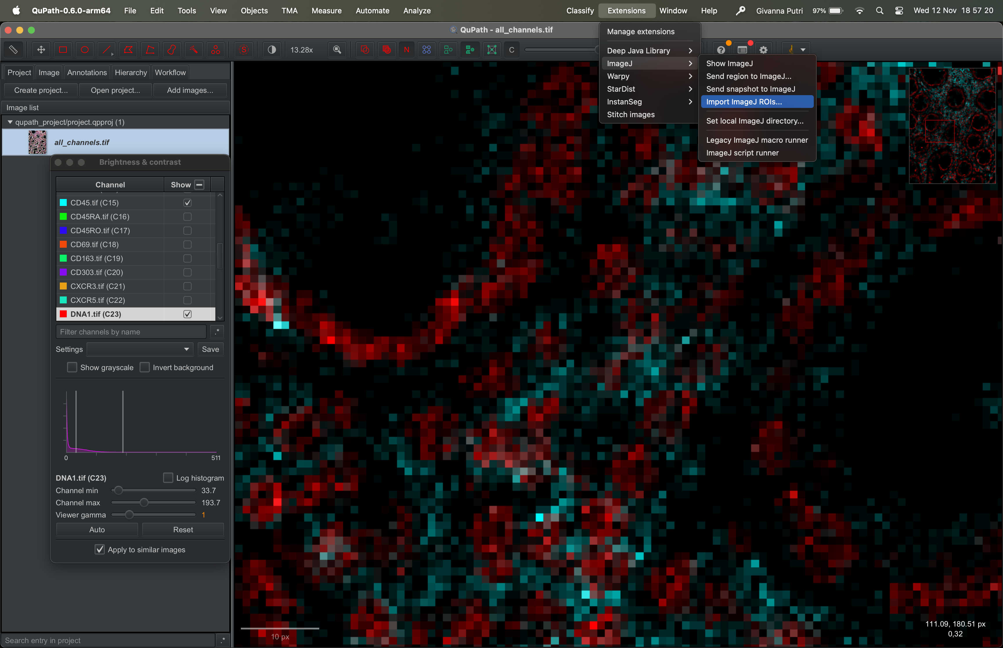
Select the zip file we exported from ImageJ and click ok. You should now get the segmentation masks overlaid over the image.
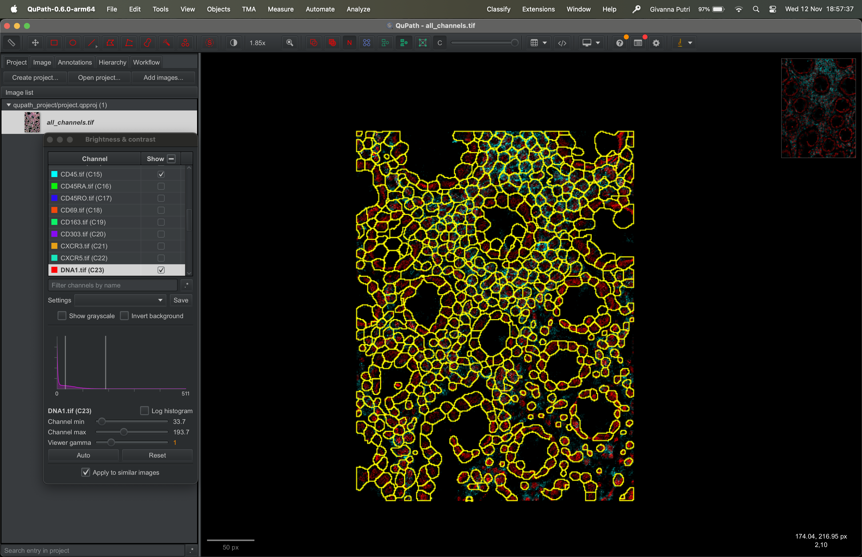
Manually modifying segmentation masks using Qupath
We can now scrutinise this segmentation result. Toggle few channels and see how it looks. Zoom in and out the tissue.
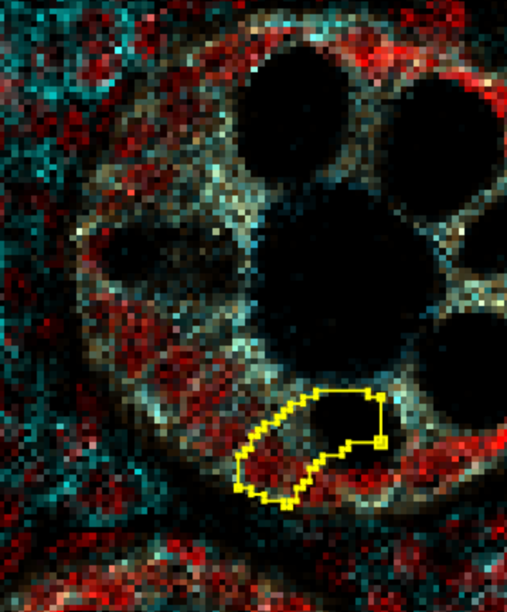
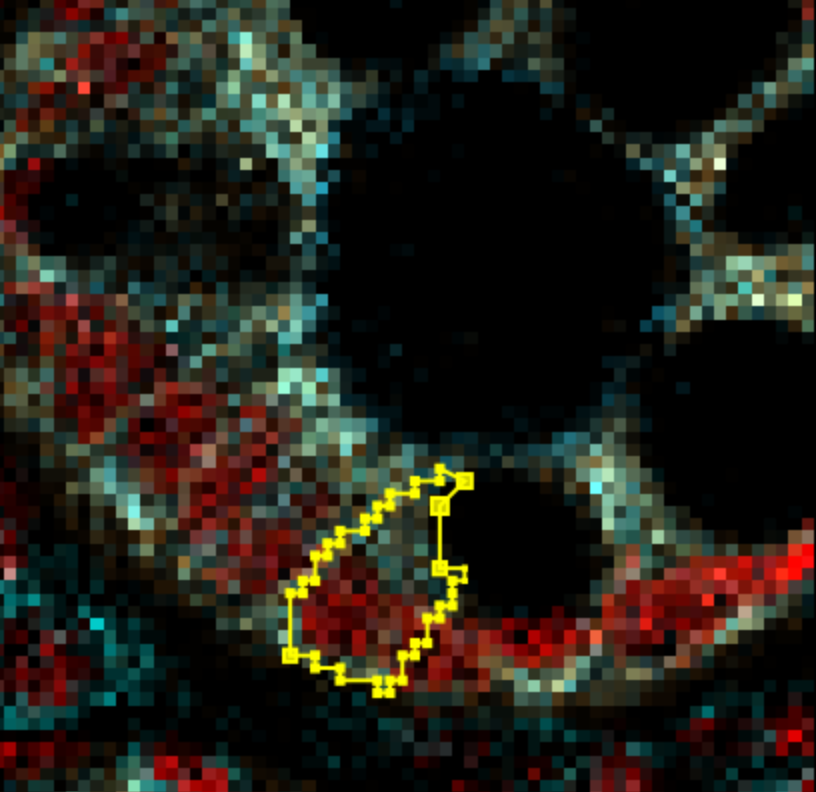
If you find a weird or just plain wrong segmentation, like below where we have cells missing DNA (red) - double clicking on a cell should focus on it. You can delete it by just pressing the delete key.
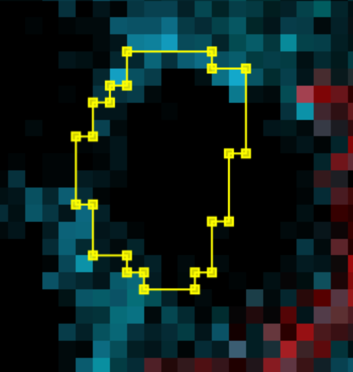
Or if you get an overzealous one like the one below, you can select it by double clicking and drag the nodes around to reshape it.
Qupath should automatically merge the nodes or create new ones as you drag them around.
Exporting segmentation masks
To do any downstream analyses using R, we need to export the segmentation masks out into a csv file that we can read in using R.
Measuring channel intensity
To do this, we need to first get Qupath to measure the intensity of each channel.
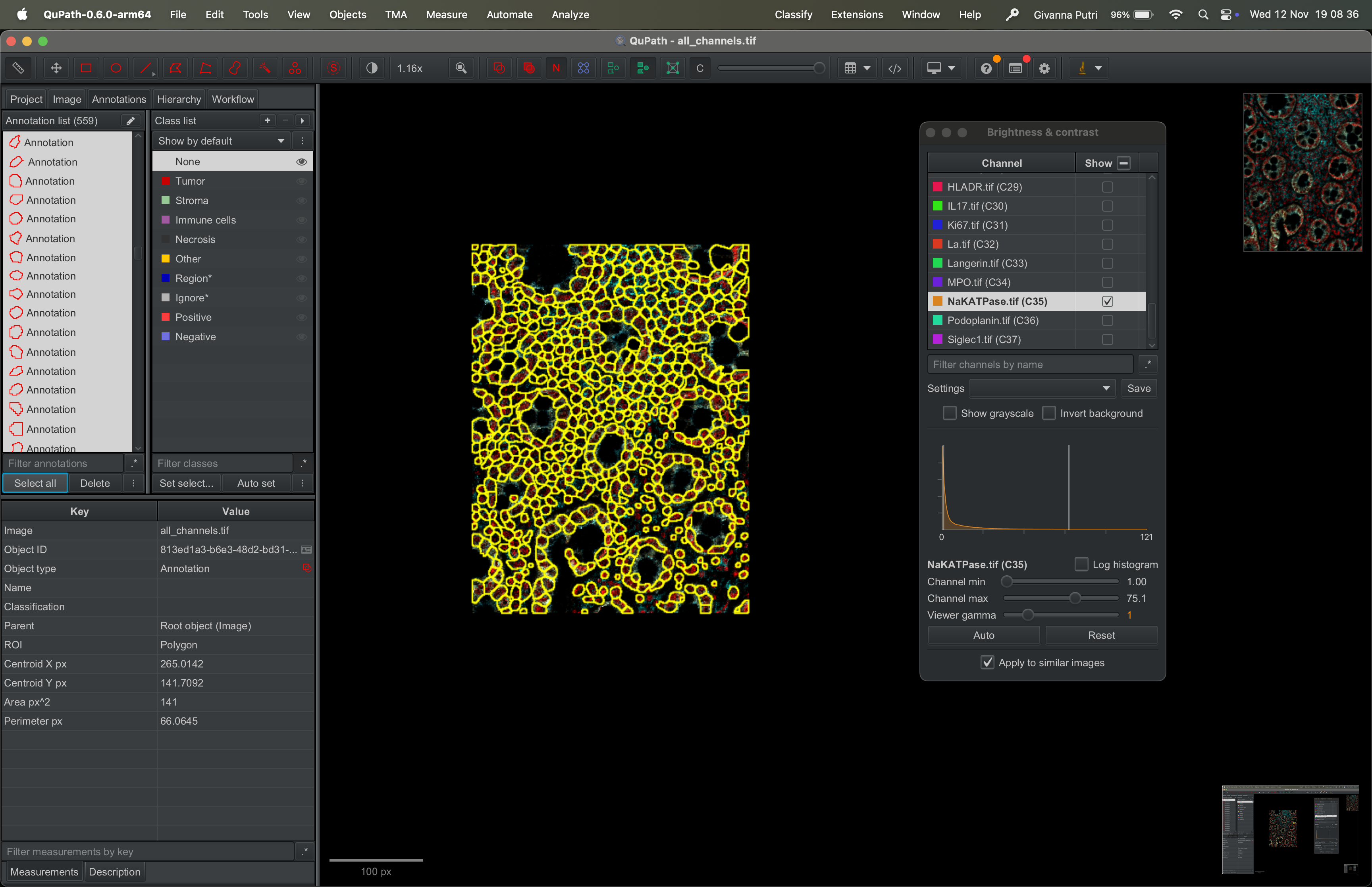
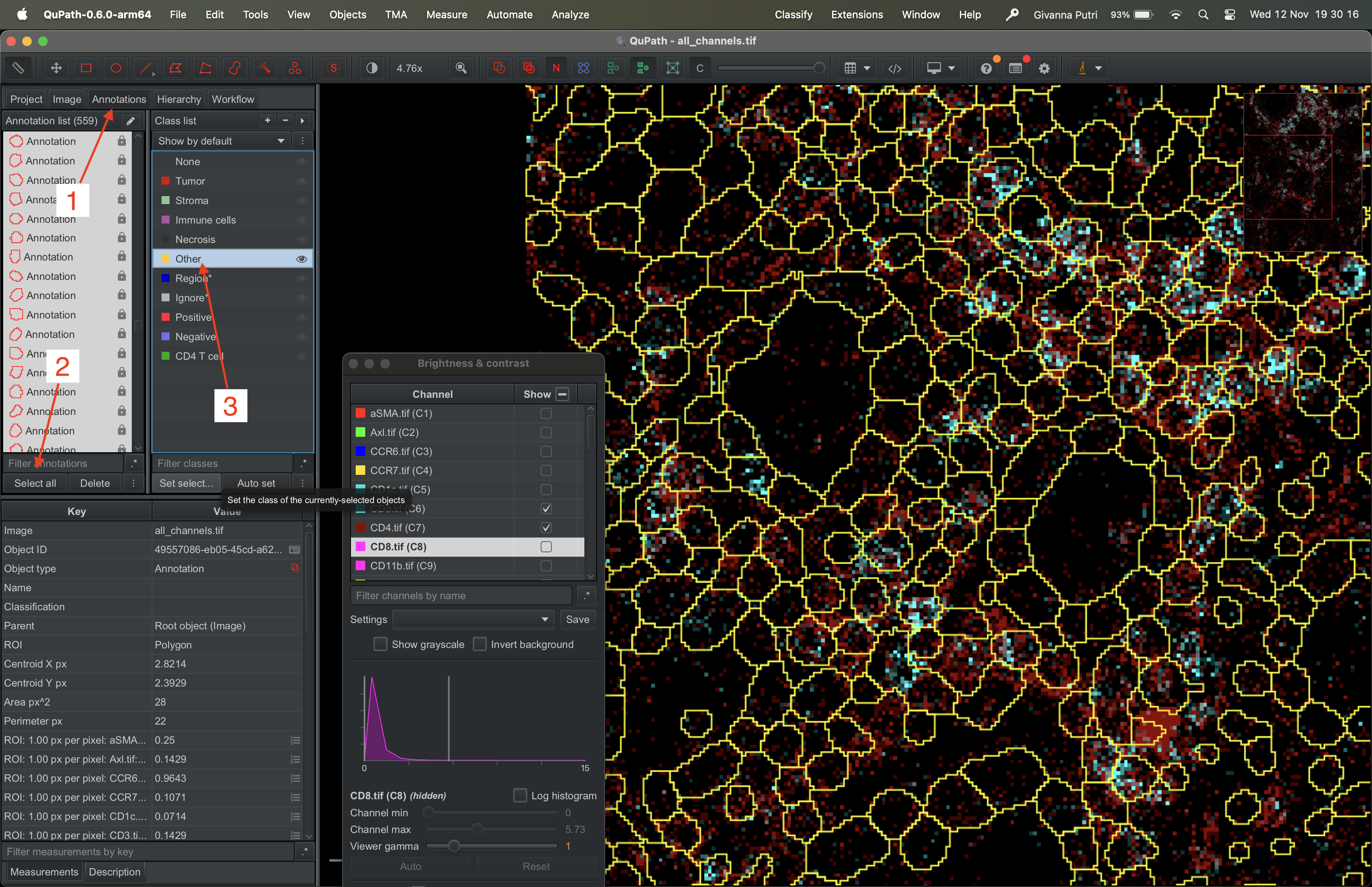
First, go to Annotations tab on the menu panel on the left and click select all.
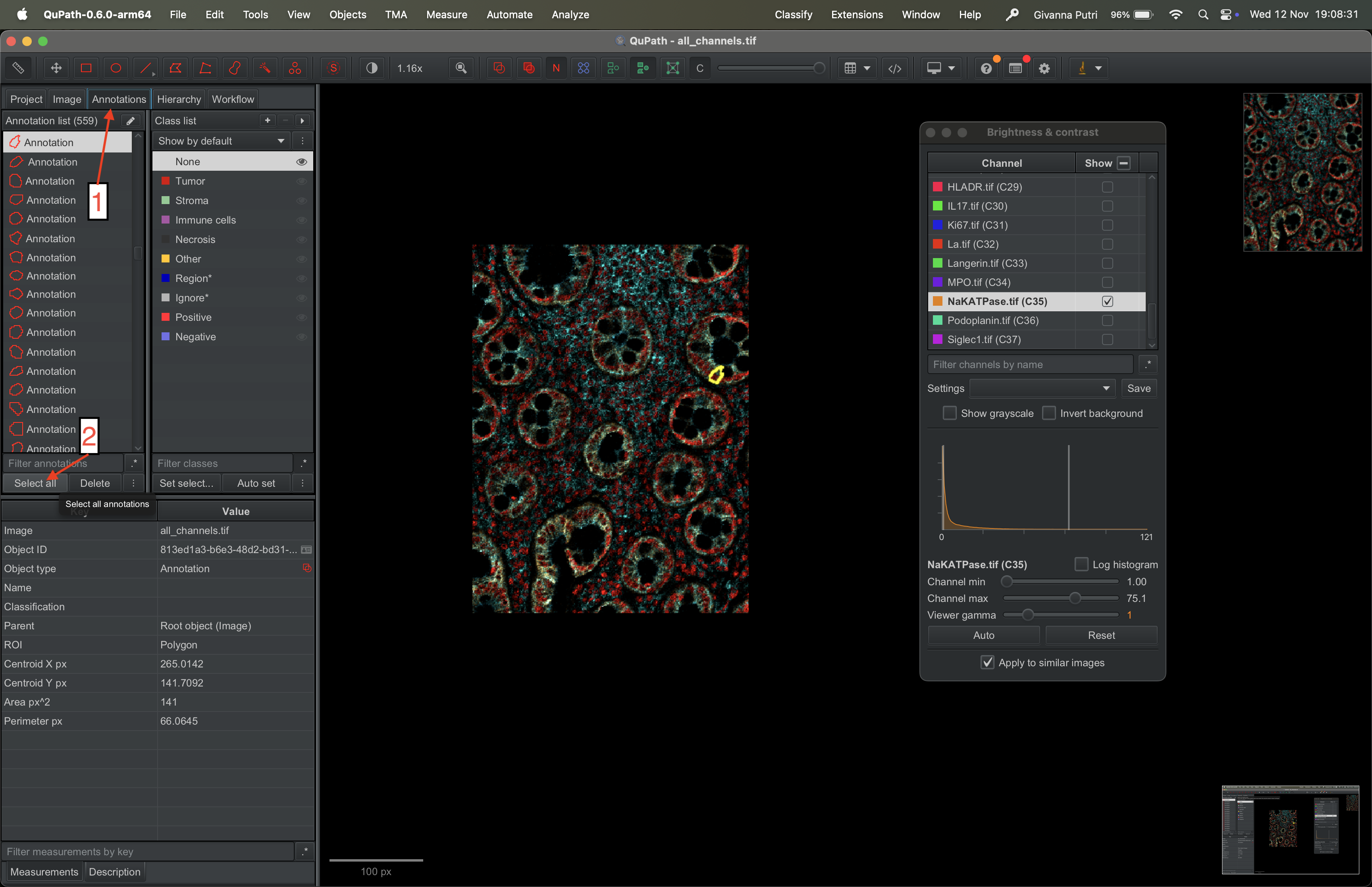
This should select all segmentation masks, like so.
Go to Analyze → Calculate Features → Add intensity features.
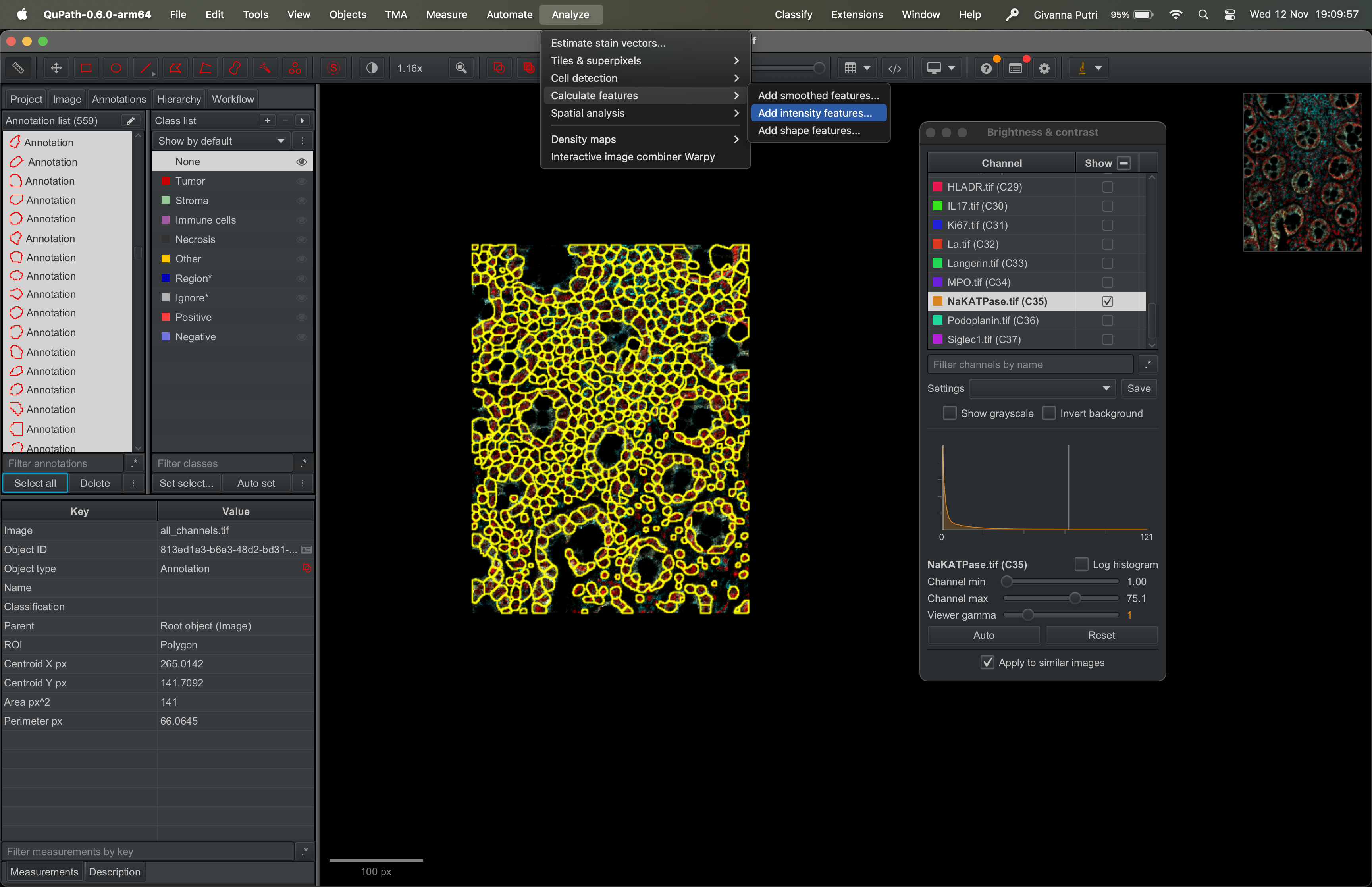
Tick all the channels one after another. Scroll down and select mean.
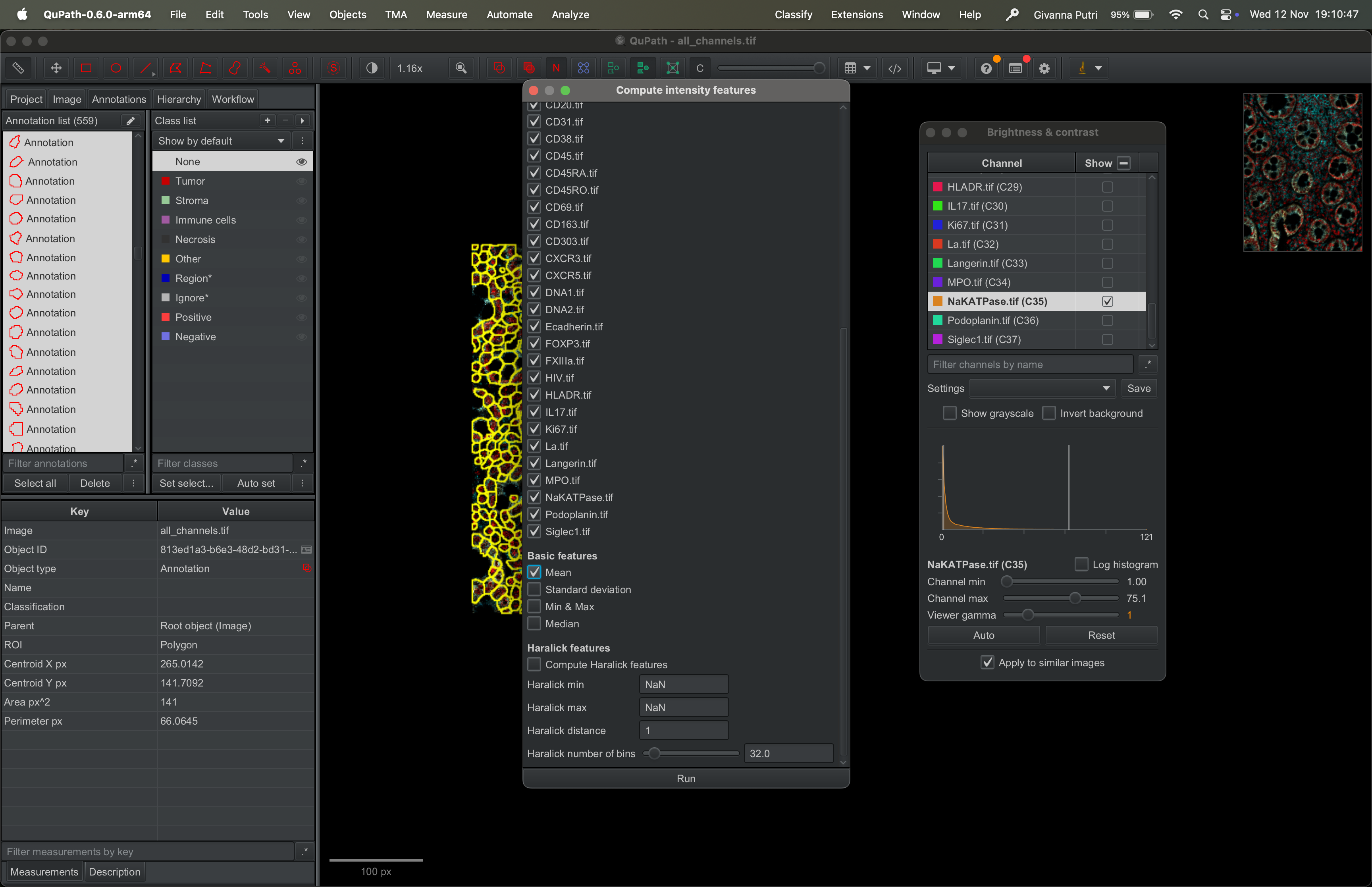
This tells Qupath to export out the mean intensity for each mask. There are other options, median, SD, min & max. If you want you can select more than one options. Then hit run.
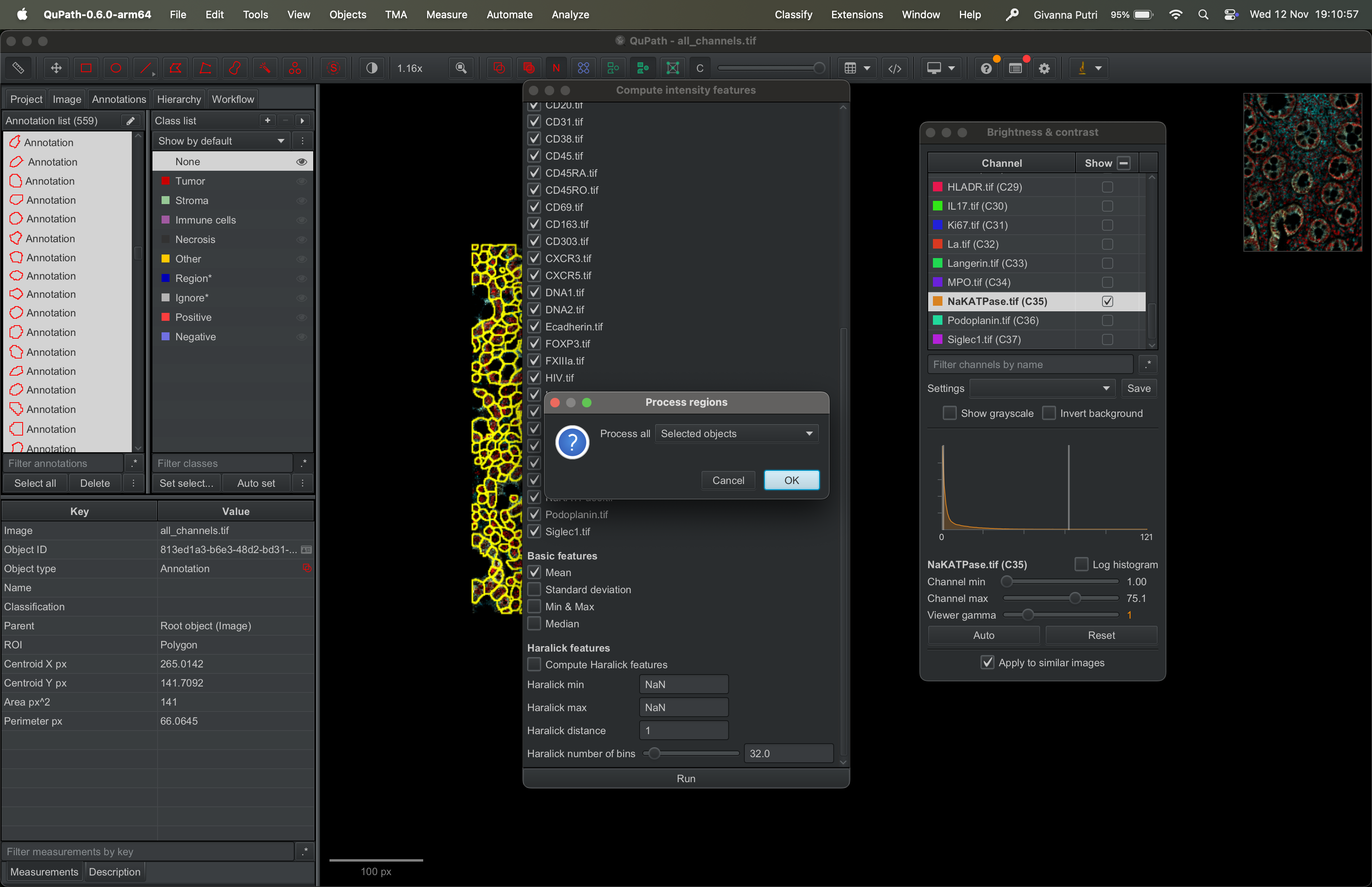
It will then ask you to what to process, select “Selected objects” then click ok.
When it finishes, the panel at bottom left should be populated with intensity measurements for all channels.
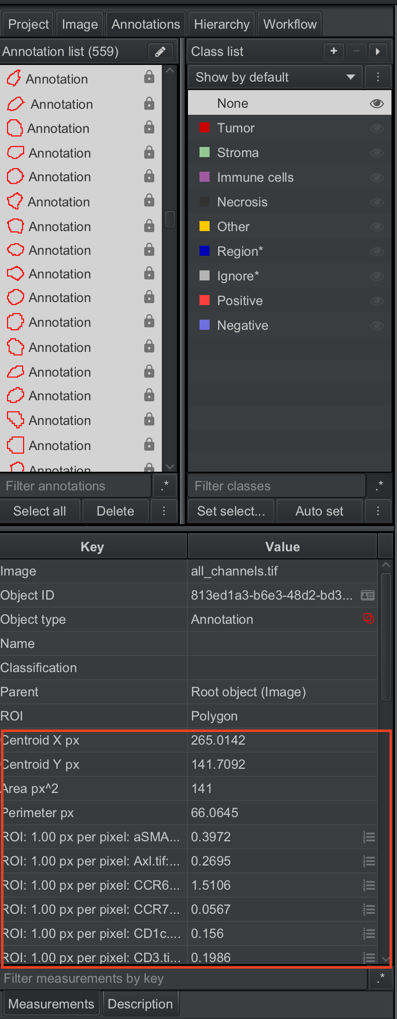
Annotating masks
When exporting masks, QuPath needs to know what masks to export. To tell it this, we need to assign an annotation to the masks.
Go to Annotations tab on the left panel, click “Select all” button on the Annotation list panel (like before). It shall highlight all the masks. Then pick “Other” on the class list panel and click “Set select…” button in the panel.
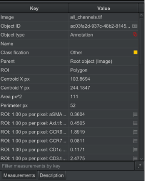
You should then see in the bottom left panel the classification row will say “other”.
You can also of course, annotate your cells by flicking through various channels, selecting individual masks and annotate them. BUT! This is best done using more traditional high dimensional approach.
However if you prefer to do it using Qupath..
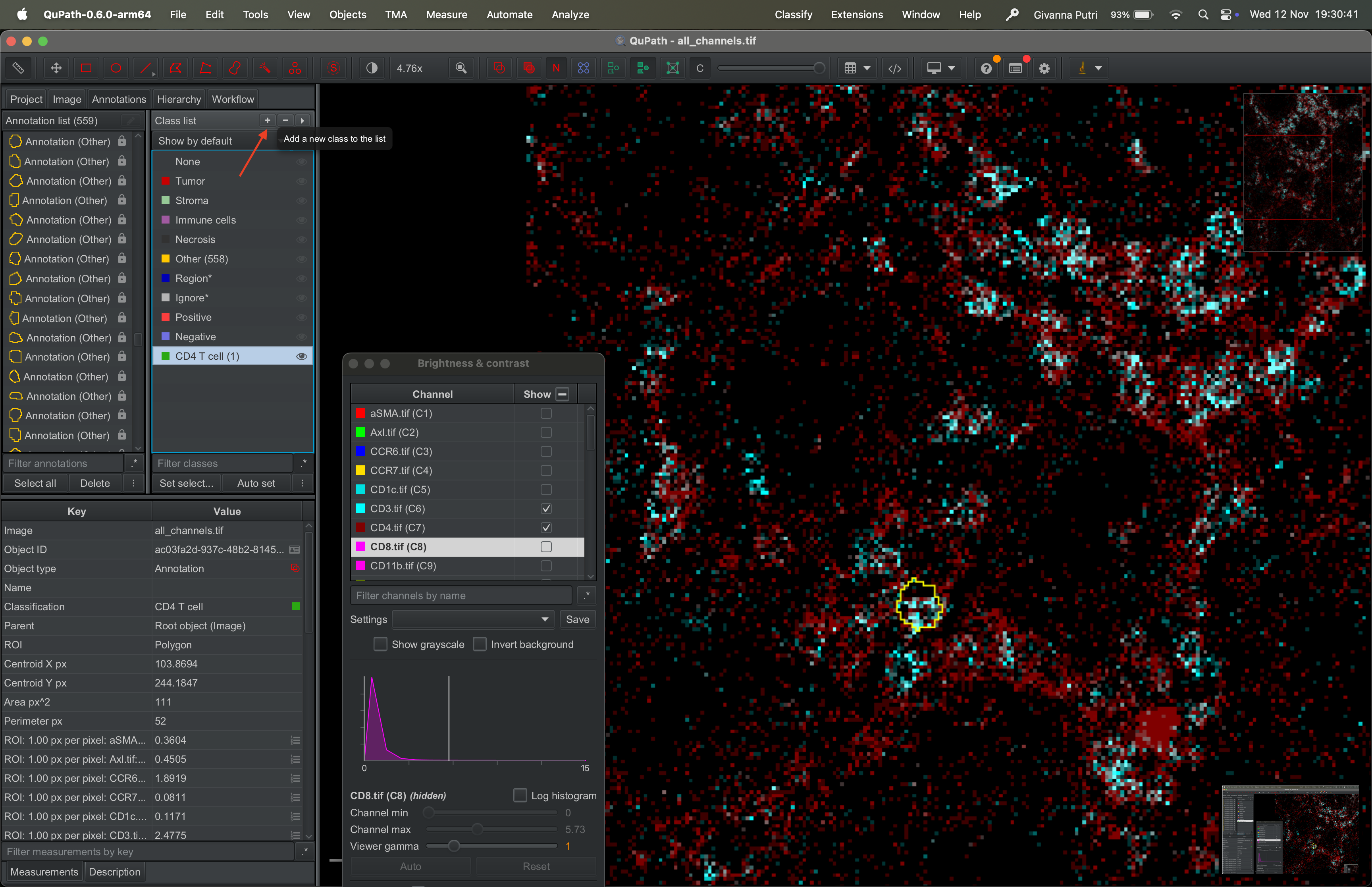
On the class list panel, click on the + button to create a new label. Say CD4 T cell.
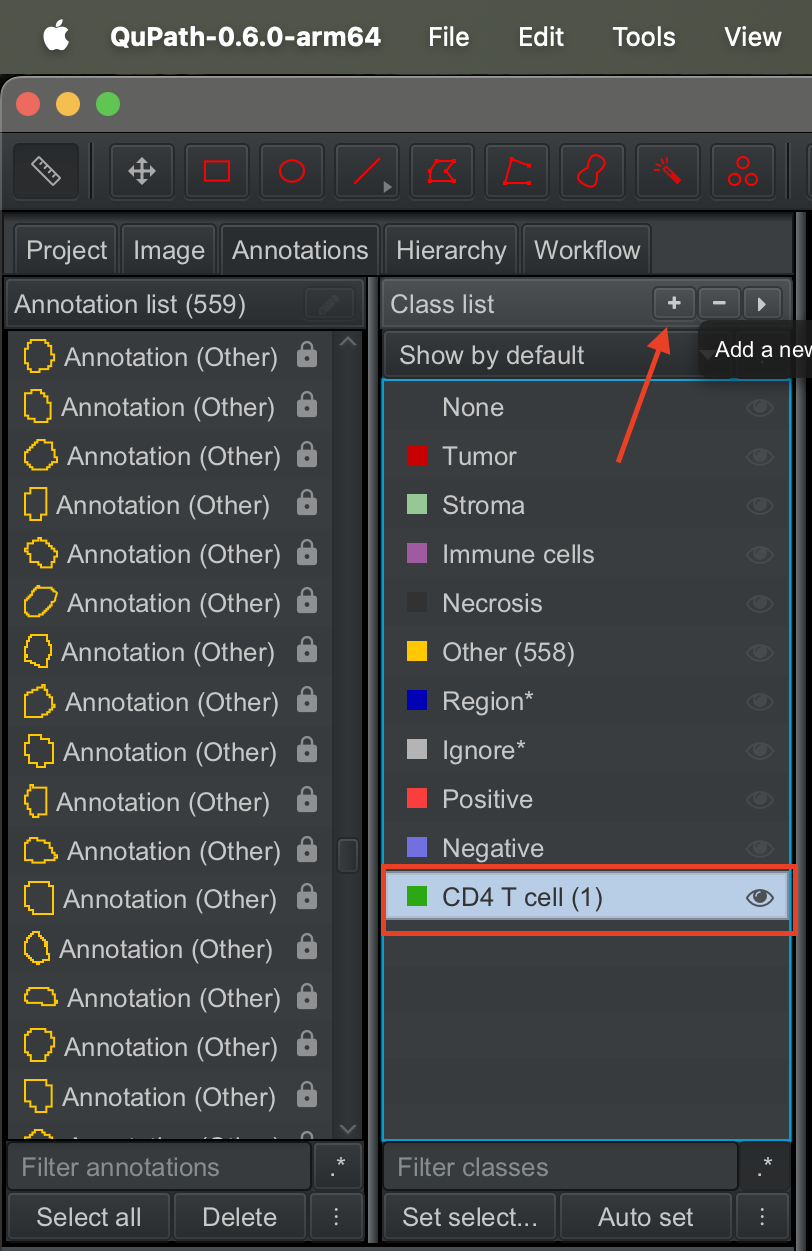
Select a mask that you think represents CD4 T cell. Then select the CD4 T cell class in the class list, then click set selected.
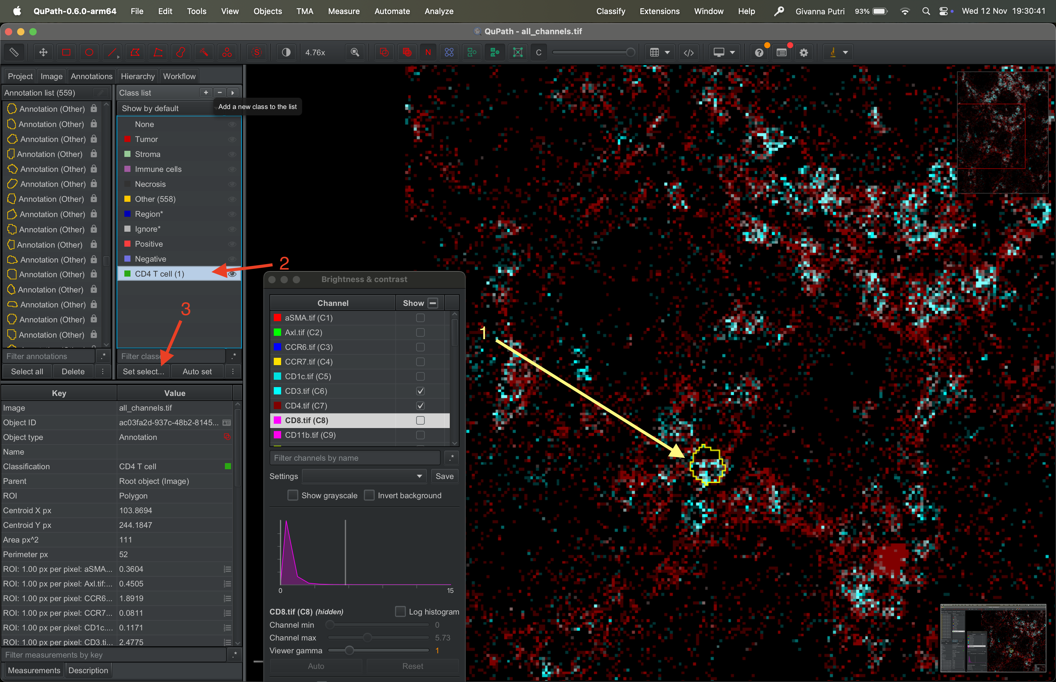
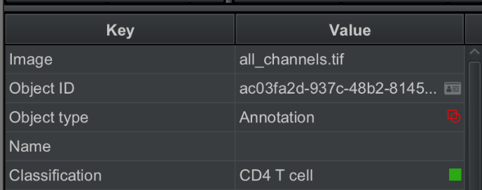
Then panel on the bottom left, should show CD4 T cell in the
classification row.
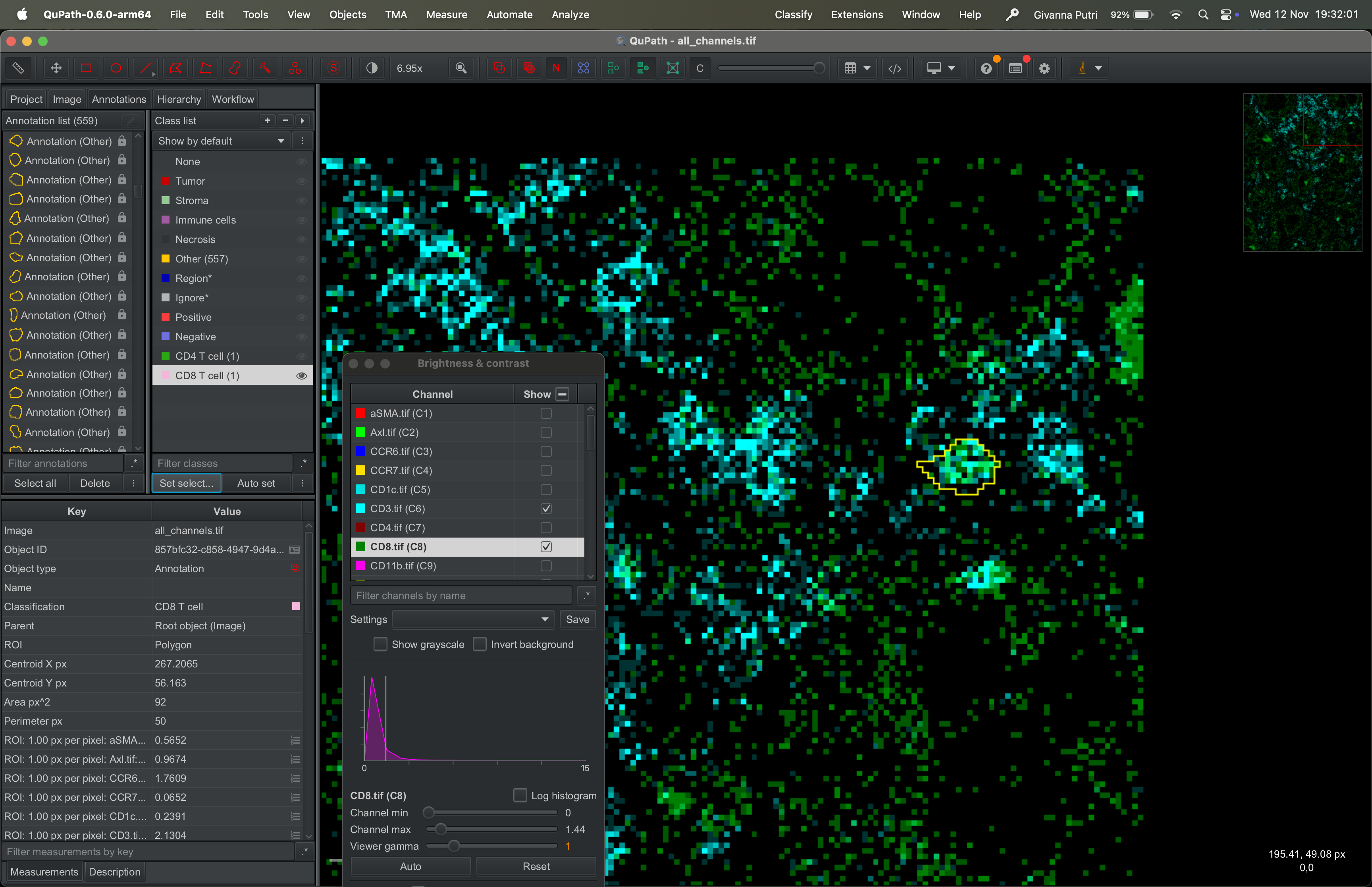
We can repeat for different class, say CD8 T cell.
Export the masks
Now we can finally export the masks.
Click “Select all” in the annotation list panel on the left, just like before. Go to Measure → Export measurements.
Select the tif file on the available panel on the left and click >> to transfer it to the right panel. Set the output file to whatever the filename you want to export it to.
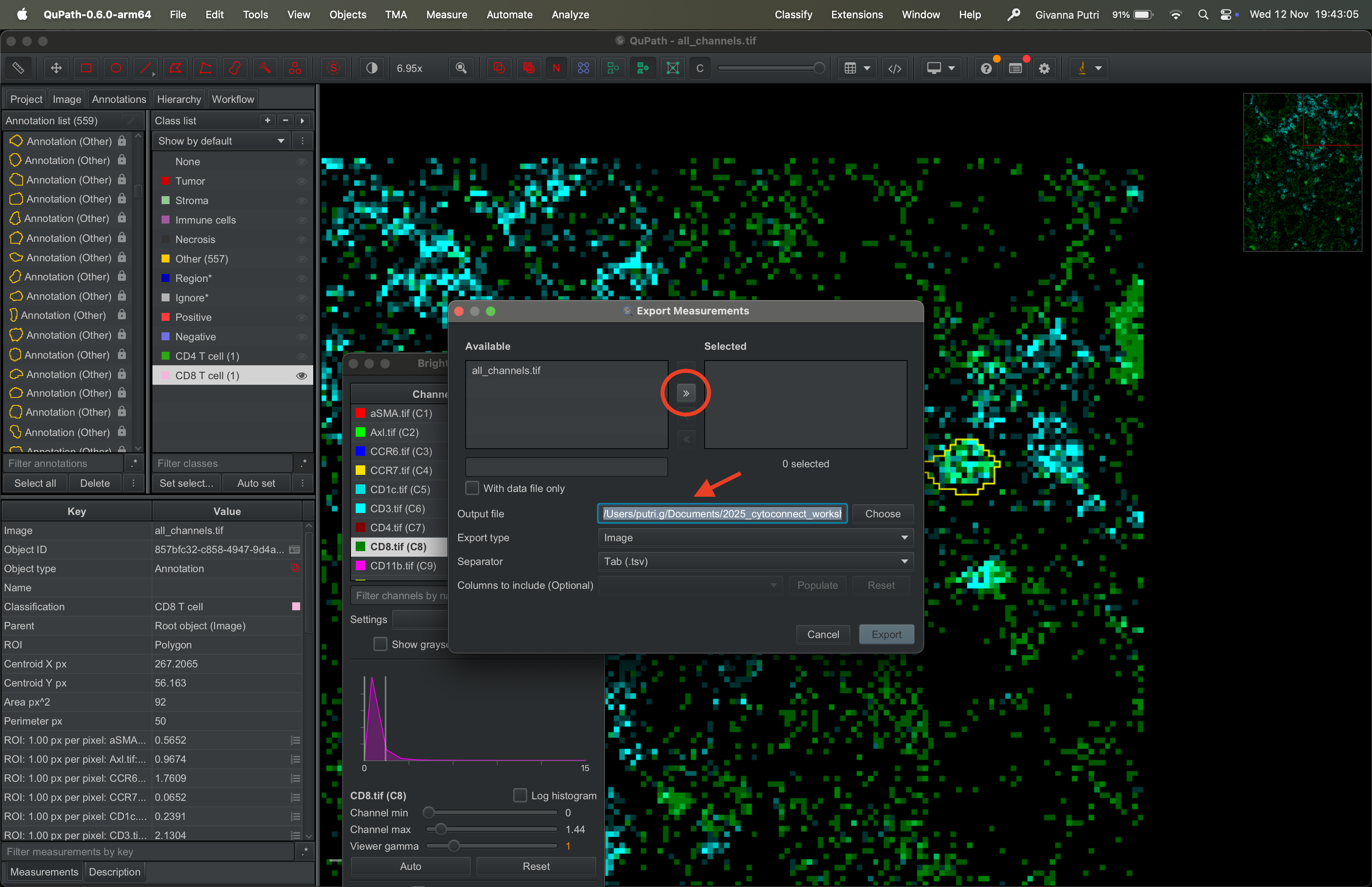
Select “Annotations” as “Export type”, and csv as “Separator”. Click the populate button.
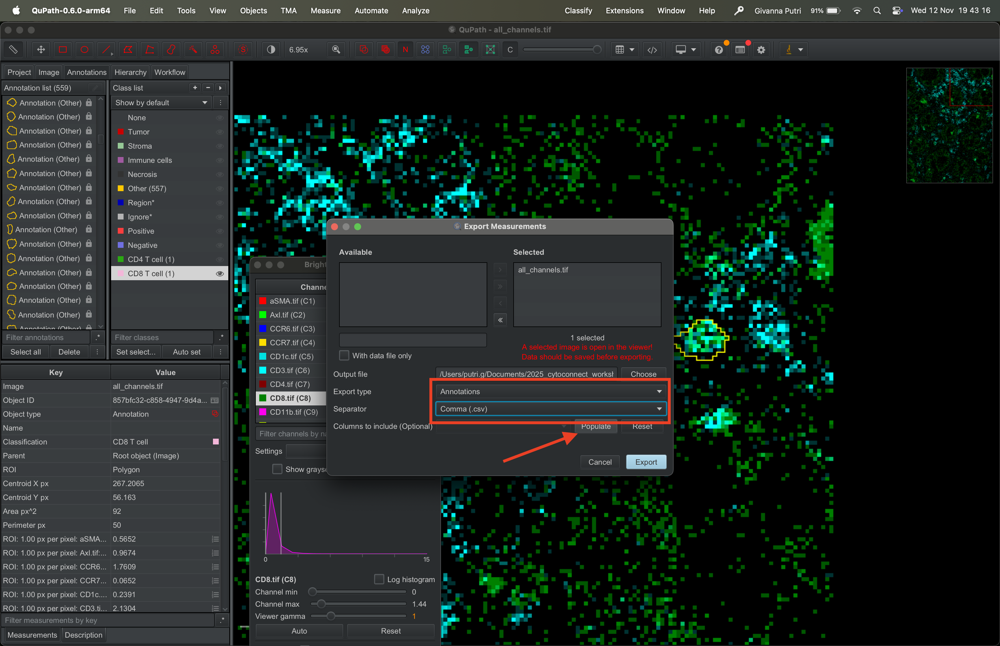
Tick everything you want to export.
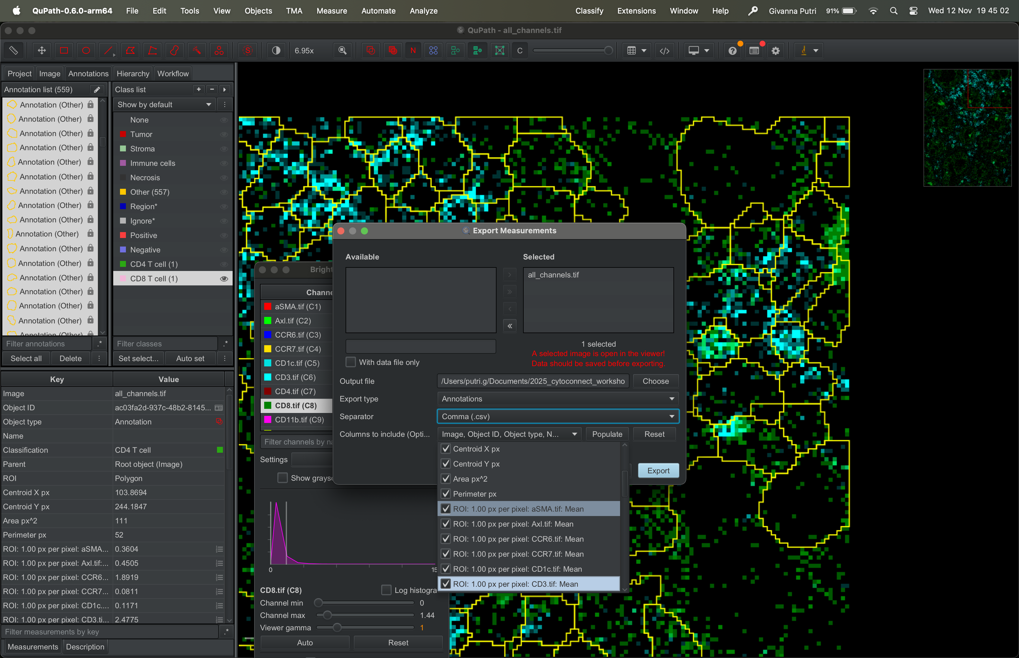
Then click export and save it to
data/imc/measurements.csv folder you created in the setup
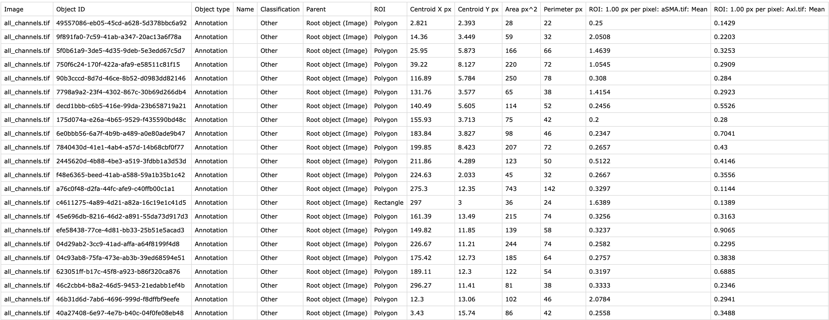
step.
You should now have a csv file like this that you can now export to R.
sessionInfo()R version 4.5.1 (2025-06-13)
Platform: aarch64-apple-darwin20
Running under: macOS Sequoia 15.5
Matrix products: default
BLAS: /Library/Frameworks/R.framework/Versions/4.5-arm64/Resources/lib/libRblas.0.dylib
LAPACK: /Library/Frameworks/R.framework/Versions/4.5-arm64/Resources/lib/libRlapack.dylib; LAPACK version 3.12.1
locale:
[1] en_US.UTF-8/en_US.UTF-8/en_US.UTF-8/C/en_US.UTF-8/en_US.UTF-8
time zone: Australia/Melbourne
tzcode source: internal
attached base packages:
[1] stats graphics grDevices utils datasets methods base
other attached packages:
[1] workflowr_1.7.2
loaded via a namespace (and not attached):
[1] vctrs_0.6.5 httr_1.4.7 cli_3.6.5 knitr_1.50
[5] rlang_1.1.6 xfun_0.53 stringi_1.8.7 processx_3.8.6
[9] promises_1.3.3 jsonlite_2.0.0 glue_1.8.0 rprojroot_2.1.1
[13] git2r_0.36.2 htmltools_0.5.8.1 httpuv_1.6.16 ps_1.9.1
[17] sass_0.4.10 rmarkdown_2.29 jquerylib_0.1.4 tibble_3.3.0
[21] evaluate_1.0.5 fastmap_1.2.0 yaml_2.3.10 lifecycle_1.0.4
[25] whisker_0.4.1 stringr_1.5.2 compiler_4.5.1 fs_1.6.6
[29] pkgconfig_2.0.3 Rcpp_1.1.0 rstudioapi_0.17.1 later_1.4.4
[33] digest_0.6.37 R6_2.6.1 pillar_1.11.0 callr_3.7.6
[37] magrittr_2.0.4 bslib_0.9.0 tools_4.5.1 cachem_1.1.0
[41] getPass_0.2-4