Visium part 3

workflowr

• Summary
• Checks
• Past versions

Last updated: 2025-11-19

Checks: 7 0

Knit directory: 2025_cytoconnect_spatial_workshop/

This reproducible R Markdown analysis was created with workflowr (version 1.7.2). The Checks tab describes the reproducibility checks that were applied when the results were created. The Past versions tab lists the development history.

---

R Markdown file: up-to-date

Great! Since the R Markdown file has been committed to the Git repository, you know the exact version of the code that produced these results.

Environment: empty

Great job! The global environment was empty. Objects defined in the global environment can affect the analysis in your R Markdown file in unknown ways. For reproduciblity it’s best to always run the code in an empty environment.

Seed: set.seed(20251002)

The command set.seed(20251002) was run prior to running the code in the R Markdown file. Setting a seed ensures that any results that rely on randomness, e.g. subsampling or permutations, are reproducible.

Session information: recorded

Great job! Recording the operating system, R version, and package versions is critical for reproducibility.

Cache: none

Nice! There were no cached chunks for this analysis, so you can be confident that you successfully produced the results during this run.

File paths: relative

Great job! Using relative paths to the files within your workflowr project makes it easier to run your code on other machines.

Repository version: cf4dc7c

Great! You are using Git for version control. Tracking code development and connecting the code version to the results is critical for reproducibility.

The results in this page were generated with repository version cf4dc7c. See the Past versions tab to see a history of the changes made to the R Markdown and HTML files.

Note that you need to be careful to ensure that all relevant files for the analysis have been committed to Git prior to generating the results (you can use wflow_publish or wflow_git_commit). workflowr only checks the R Markdown file, but you know if there are other scripts or data files that it depends on. Below is the status of the Git repository when the results were generated:

Ignored files:
    Ignored:    .DS_Store
    Ignored:    data/.DS_Store
    Ignored:    data/imc/
    Ignored:    data/visium/

Note that any generated files, e.g. HTML, png, CSS, etc., are not included in this status report because it is ok for generated content to have uncommitted changes.

---

These are the previous versions of the repository in which changes were made to the R Markdown (analysis/visium_03.Rmd) and HTML (docs/visium_03.html) files. If you’ve configured a remote Git repository (see ?wflow_git_remote), click on the hyperlinks in the table below to view the files as they were in that past version.

File	Version	Author	Date	Message
Rmd	cf4dc7c	Givanna Putri	2025-11-19	wflow_publish(c("analysis/index.Rmd", "analysis/visium_01.Rmd",
html	8da421e	Givanna Putri	2025-10-02	Build site.
Rmd	383f3f1	Givanna Putri	2025-10-02	First publish for website

---

Introduction

In this part of the workshop, we will learn how to create some spatial plots using Seurat and how to customise them.

Load packages and data

library(Seurat)
library(qs2)
library(ggplot2)
library(scales)

We will be using the Seurat object that we have QCed and normalised in part 2.

dat <- qs_read(file.path(here::here(), "data", "visium", "extdata", "visium_seurat_qced_norm.qs2"))
dat

An object of class Seurat 
35982 features across 3959 samples within 2 assays 
Active assay: SCT (17991 features, 3000 variable features)
 3 layers present: counts, data, scale.data
 1 other assay present: Spatial
 1 spatial field of view present: slice1

SpatialFeaturePlot

SpatialFeaturePlot is a function in Seurat that allows you to plot a feature (e.g., the expression of a gene) of the spots over the image of the tissue.

For example, let’s plot the expression of CD3D gene of our data.

SpatialFeaturePlot(dat, features = "CD3D")

Warning: `aes_string()` was deprecated in ggplot2 3.0.0.
ℹ Please use tidy evaluation idioms with `aes()`.
ℹ See also `vignette("ggplot2-in-packages")` for more information.
ℹ The deprecated feature was likely used in the Seurat package.
  Please report the issue at <https://github.com/satijalab/seurat/issues>.
This warning is displayed once every 8 hours.
Call `lifecycle::last_lifecycle_warnings()` to see where this warning was
generated.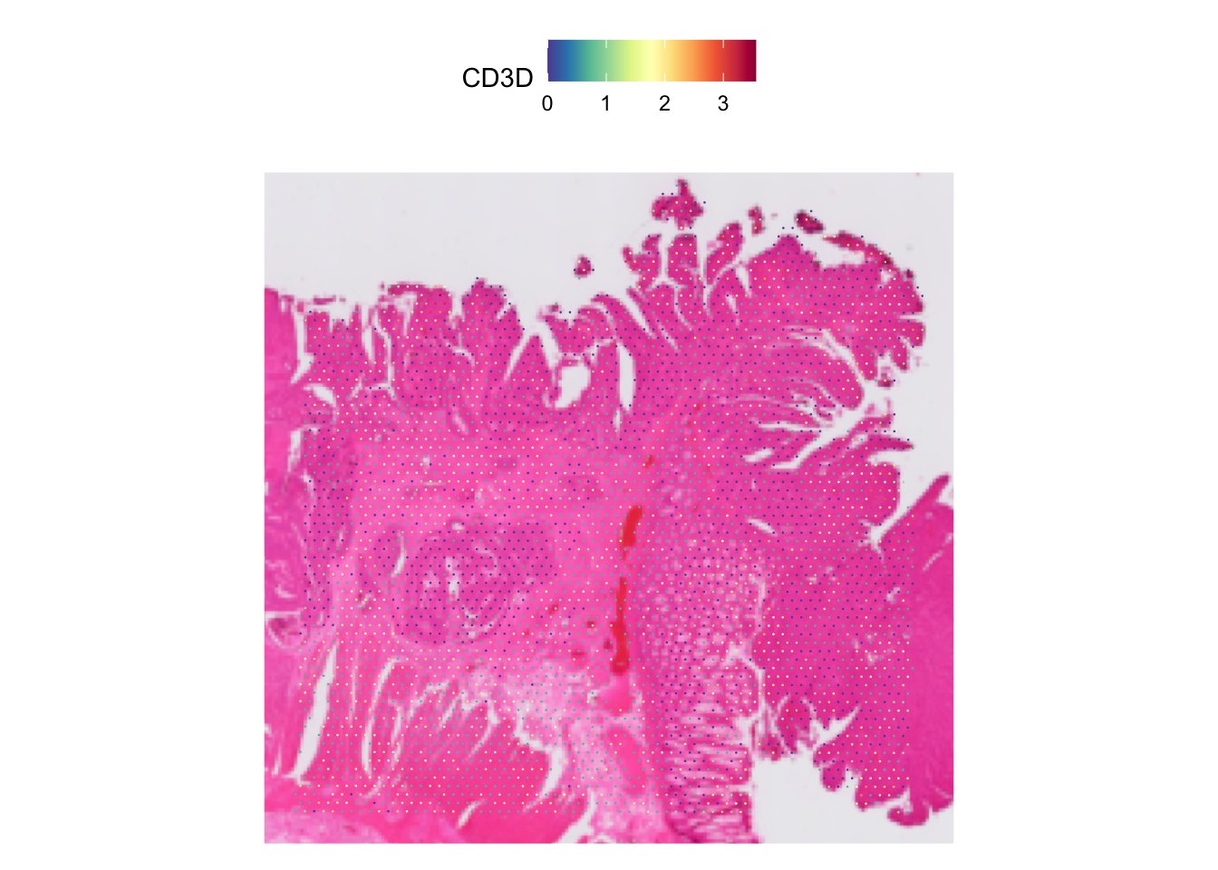

Past versions of unnamed-chunk-3-1.png

Version	Author	Date
8da421e	Givanna Putri	2025-10-02

Often, the spots may look too small, like in this case. We can increase it by increasing the pt.size.factor parameter.

# store it so we can use the same number later on
pt_size <- 5
SpatialFeaturePlot(dat, features = "CD3D", pt.size.factor = pt_size)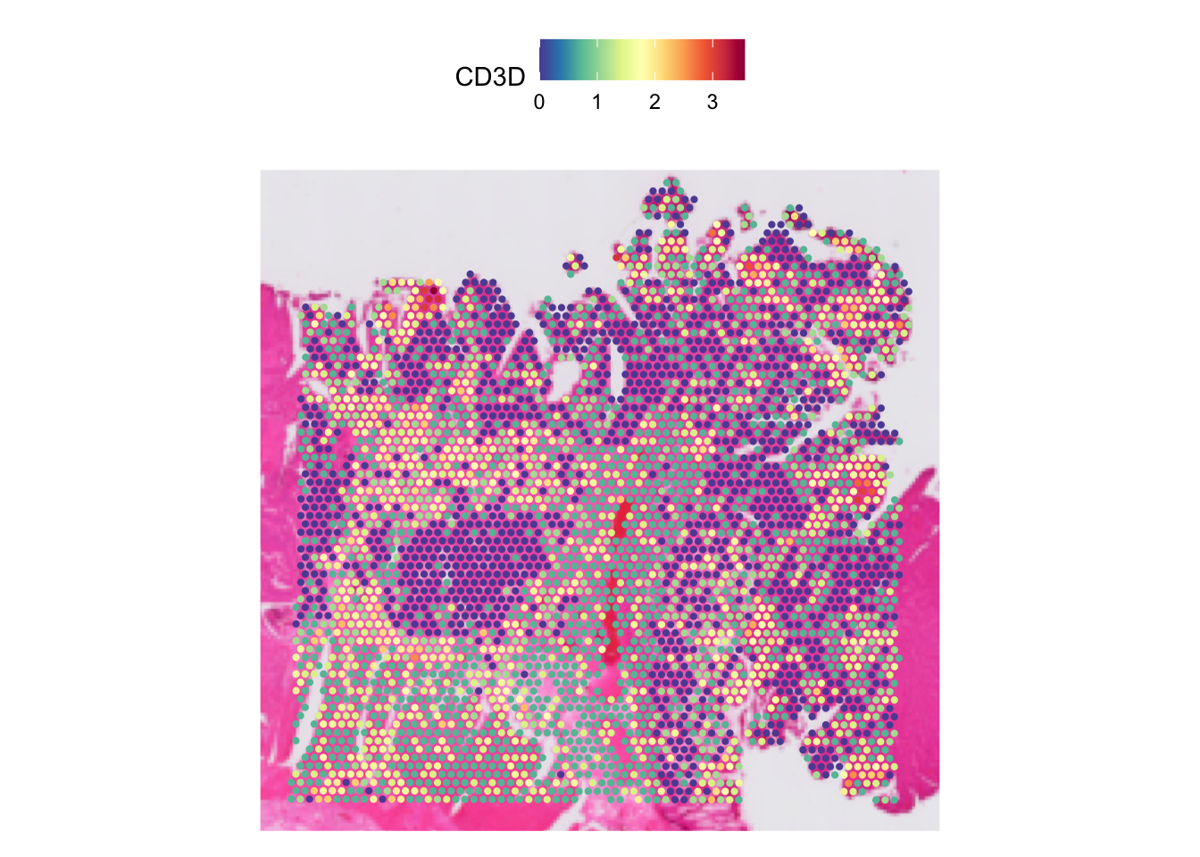

Past versions of unnamed-chunk-4-1.png

Version	Author	Date
8da421e	Givanna Putri	2025-10-02

We can also adjust the opacity of the spots and the image underneath it by tuning the alpha and image.alpha parameter accordingly. The higher the number, the less opaque the spots and image will be.

# Dimming the spots
SpatialFeaturePlot(dat, features = "CD3D", pt.size.factor = pt_size, alpha = 0.3)

Past versions of unnamed-chunk-5-1.png

Version	Author	Date
8da421e	Givanna Putri	2025-10-02

# Dimming the image
SpatialFeaturePlot(dat, features = "CD3D", pt.size.factor = pt_size, image.alpha = 0.5)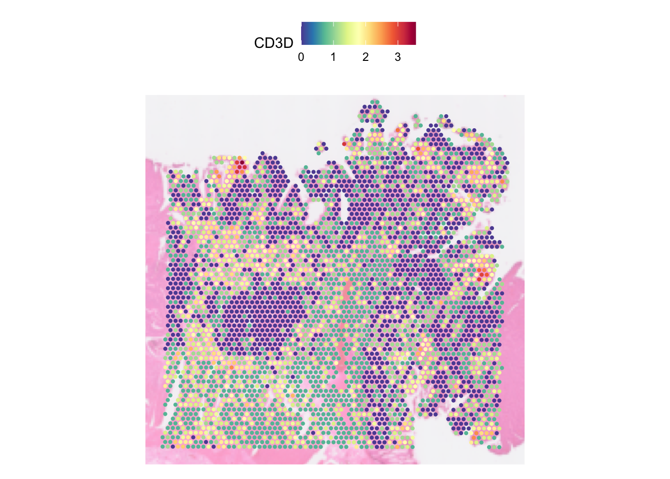

Past versions of unnamed-chunk-5-2.png

Version	Author	Date
8da421e	Givanna Putri	2025-10-02

# Completely removing the image
SpatialFeaturePlot(dat, features = "CD3D", pt.size.factor = pt_size, image.alpha = 0)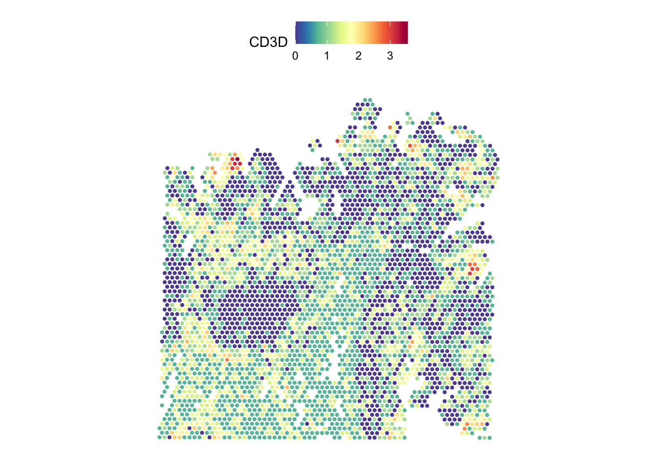

Past versions of unnamed-chunk-5-3.png

Version	Author	Date
8da421e	Givanna Putri	2025-10-02

If a range is passed onto the alpha parameter, it will alter the minimum and maximum opacity. This is handy if you want to accentuate the higher expression as we can lower the minimum opacity (which defaulted to 1) and increase the maximum opacity.

SpatialFeaturePlot(dat, features = "CD3D", pt.size.factor = 5, 
                   image.alpha = 0.5, alpha = c(0.5, 3))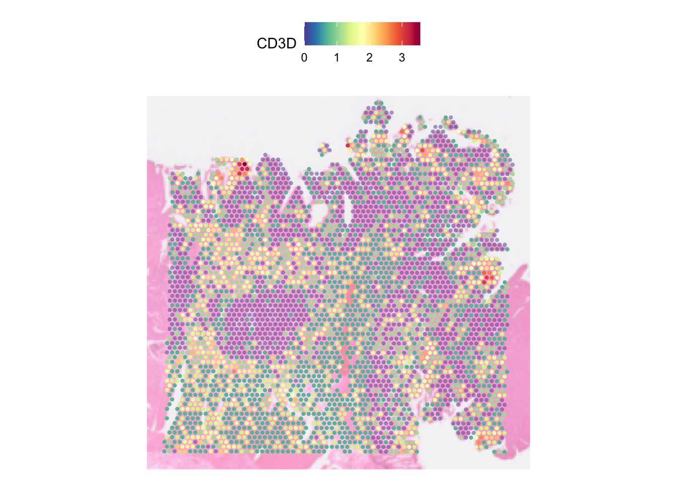

Past versions of unnamed-chunk-6-1.png

Version	Author	Date
8da421e	Givanna Putri	2025-10-02

In the plot above, each spot is coloured by the expression of CD3D gene. Notably, because the active assay of the data was set to SCT before we run SpatialFeaturePlot, the CD3D expression we plotted above is not the raw UMI count, but rather the count that has been normalised using SCTransformed, stored in the data layer.

We can run the function on the raw unnormalised count by changing the default assay and setting the slot parametr to the count layer:

DefaultAssay(dat) <- "Spatial"
SpatialFeaturePlot(dat, features = "CD3D", pt.size.factor = pt_size, image.alpha = 0.5,
                   slot = "count")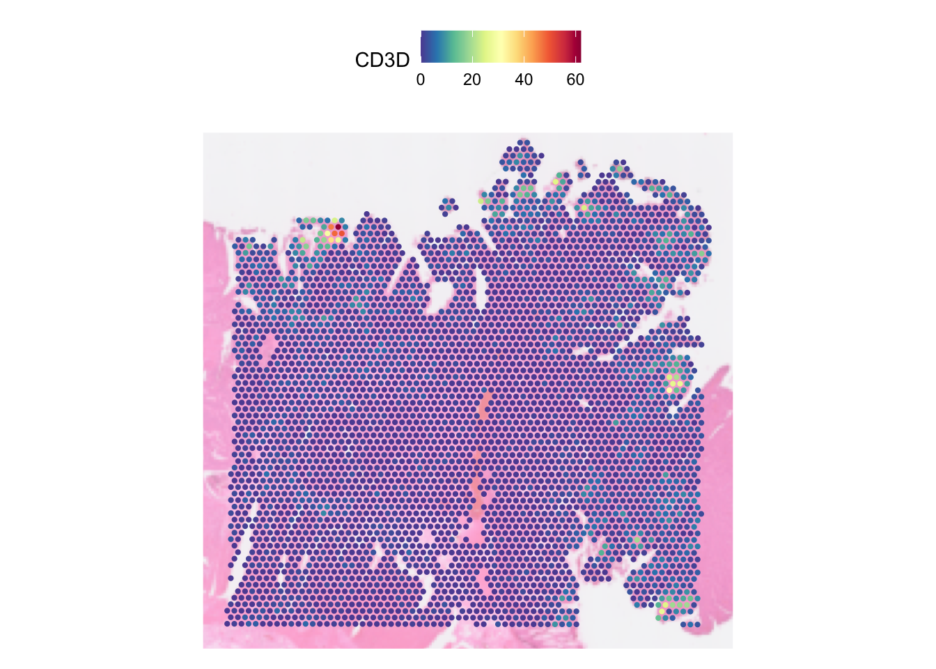

Past versions of unnamed-chunk-7-1.png

Version	Author	Date
8da421e	Givanna Putri	2025-10-02

In one SpatialFeaturePlot call, we can visualise multiple features. E.g., let’s visualise four genes, CD3D, CD3G, CD4, CD8A, :

DefaultAssay(dat) <- "SCT"
SpatialFeaturePlot(dat, pt.size.factor = 5, 
                   image.alpha = 0.5, features = c("CD3D", "CD3G", "CD4", "CD8A"))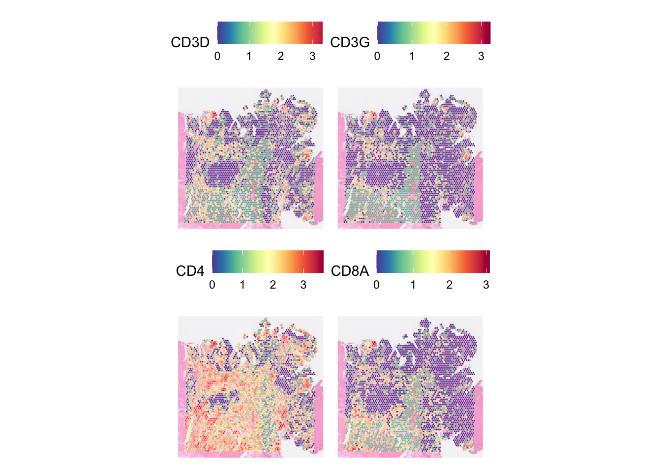

Past versions of unnamed-chunk-8-1.png

Version	Author	Date
8da421e	Givanna Putri	2025-10-02

You can set how many columns do you want to spread the images across by specifying the parameter ncol.

SpatialFeaturePlot(dat, pt.size.factor = 5, 
                   image.alpha = 0.5, 
                   features = c("CD3D", "CD3G", "CD4", "CD8A"), ncol = 4)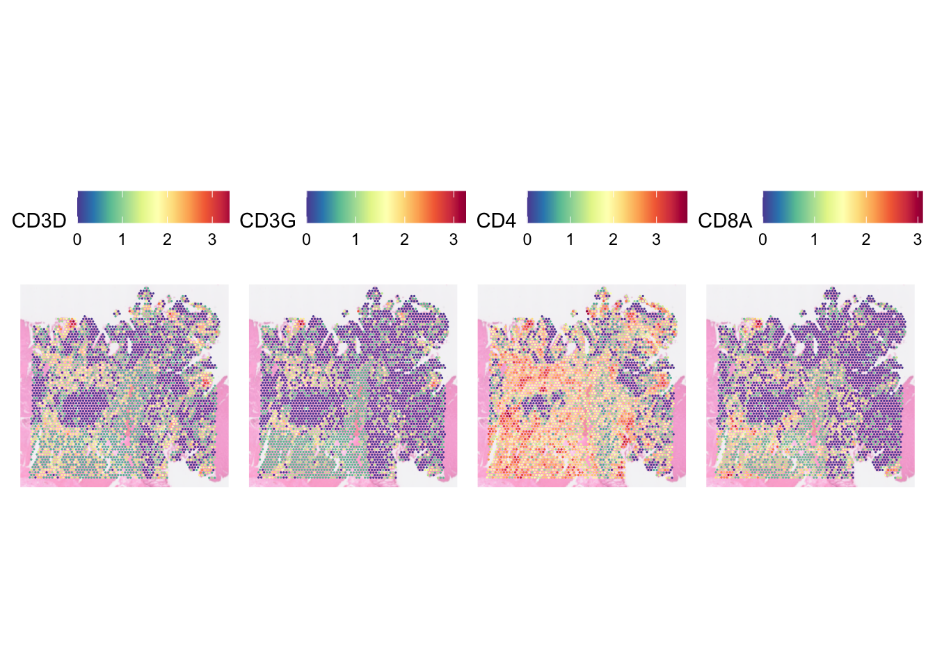

Past versions of unnamed-chunk-9-1.png

Version	Author	Date
8da421e	Givanna Putri	2025-10-02

By default, the plot will focus on the the area of the tissue where the spots are. Disabling this by setting crop to FALSE will show the entire tissue.

SpatialFeaturePlot(dat, features = "CD3D", crop=FALSE, image.alpha = 0.5, 
                   pt.size.factor = 3)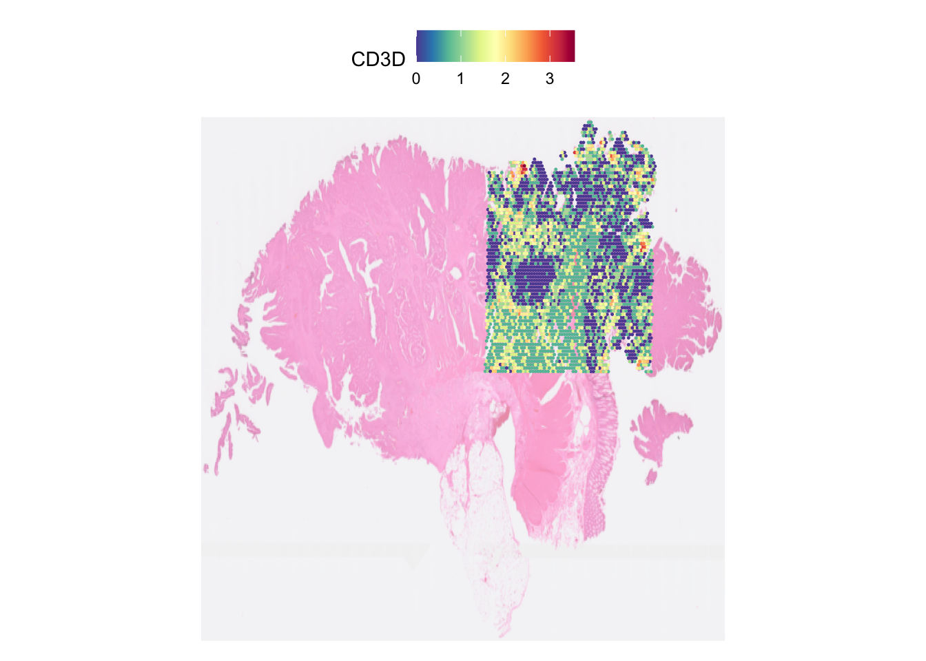

Past versions of unnamed-chunk-10-1.png

Version	Author	Date
8da421e	Givanna Putri	2025-10-02

SpatialDimPlot

SpatialDimPlot is different from SpatialFeaturePlot in that it allows us to visualise qualitative features.

For example, let’s visualise the spot by the patient ID metadata we added in part 1 before.

SpatialDimPlot(dat, group.by = 'patient_id', pt.size.factor = pt_size,
               image.alpha = 0.5)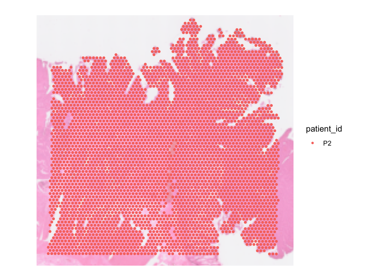

Past versions of unnamed-chunk-11-1.png

Version	Author	Date
8da421e	Givanna Putri	2025-10-02

There are some parameters that are shared between SpatialDimPlot and SpatialFeaturePlot, like pt.size.factor, image.alpha, alpha

We can override the spot colour by setting the cols parameter with a named vector mapping the discrete category in the data against the colour. To visualise this, let’s pretend we have 3 patients in our data.

# pretend we have three patients in the data
dat[[]]$pretend_patient_id <- c(
  rep("Adam", 3000),
  rep("Jane", 700),
  rep("Clare", 259)
)

SpatialDimPlot(dat, group.by = 'pretend_patient_id', 
               pt.size.factor = pt_size, image.alpha = 0.5,
               cols = c("Adam" = "#0096FF", "Jane" = "orange", "Clare" = "#023020"))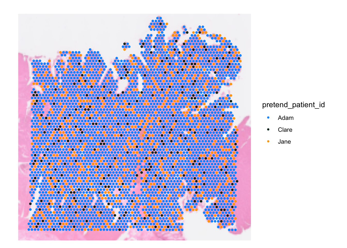

Past versions of unnamed-chunk-12-1.png

Version	Author	Date
8da421e	Givanna Putri	2025-10-02

We can also highlight only spots that belong to certain group and grey out the rest. E.g. let’s discretise spots based on their CD3D expression

SpatialDimPlot(dat, pt.size.factor = pt_size, image.alpha = 0.3,
               cells.highlight =  list(
                 "CD3pos" = WhichCells(dat, expression = CD3D > 2),
                 "CD3neg" = WhichCells(dat, expression = CD3D <= 2)),
               cols.highlight = c(
                 "CD3pos" = "yellow", 
                 "CD3neg" = "grey70"))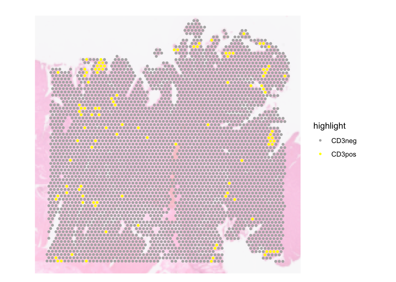

Past versions of unnamed-chunk-13-1.png

Version	Author	Date
8da421e	Givanna Putri	2025-10-02

We can also split the image such that we have 1 panel each for each group.

SpatialDimPlot(dat, pt.size.factor = pt_size, image.alpha = 0.3,
               cells.highlight =  list(
                 "CD3pos" = WhichCells(dat, expression = CD3D > 2),
                 "CD3neg" = WhichCells(dat, expression = CD3D <= 2)),
               cols.highlight = c("yellow", "grey70"),
               facet.highlight = TRUE)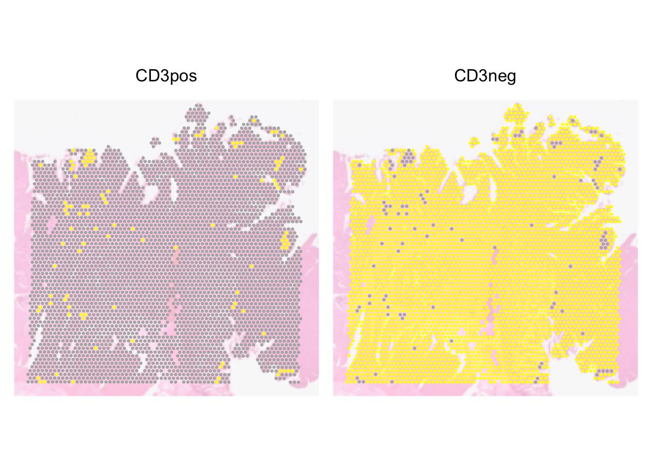

Past versions of unnamed-chunk-14-1.png

Version	Author	Date
8da421e	Givanna Putri	2025-10-02

Further customising the plots

Both SpatialFeaturePlot and SpatialDimPlot will return a ggplot object, which we can modify using the functions and notations built into the ggplot2 package.

As an example, let’s update a feature plot showing CD3D expression such that we:

1. Use the viridis colour scheme.
2. Rename CD3D to CD3D SCTransformed exp
3. Have a black background and white axes

# Default SpatialFeature Plot
plt_dark_bg <- SpatialFeaturePlot(
  dat, 
  features = "CD3D",
  pt.size.factor = pt_size,
  image.alpha = 0
) 

# 1) Overriding the colour scheme to viridis
plt_dark_bg <- plt_dark_bg + scale_fill_viridis_c(option = 'viridis')

Scale for fill is already present.
Adding another scale for fill, which will replace the existing scale.

# 2) Rename `CD3D` to `CD3D SCTransformed exprssion`
plt_dark_bg <- plt_dark_bg + labs(fill='CD3D SCTransformed exp') 

# 3) Have a black background and white axes
plt_dark_bg <- plt_dark_bg +
  theme_minimal() + 
  theme(
  legend.text = element_text(colour = "white"),
  legend.title = element_text(colour = "white"),
  legend.background = element_rect(fill = "black"),
  plot.background = element_rect(fill = "black"),
  panel.grid = element_blank(),
  axis.text = element_text(colour = "white"),
  axis.line = element_line(colour = "white")
) 
plt_dark_bg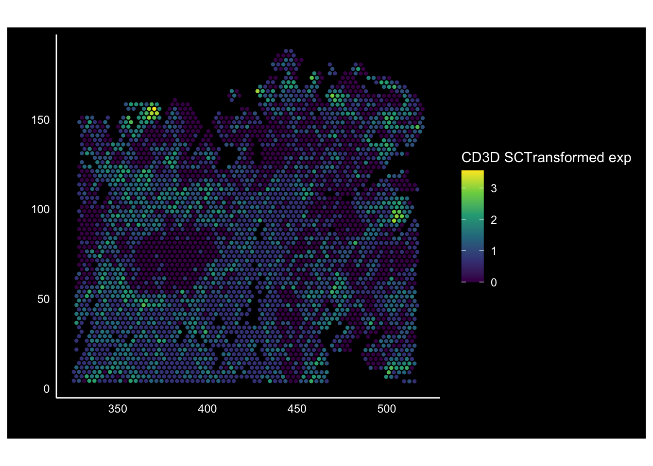

Past versions of unnamed-chunk-15-1.png

Version	Author	Date
8da421e	Givanna Putri	2025-10-02

Since the plot is a ggplot object, we can export them using either the export button in Rstudio’s panel, or the ggsave function:

ggsave(filename="visium/data/spatial_plot_darkbg.png", plot=plt_dark_bg)

---

Customising SpatialFeaturePlot with multiple features

---

When there are multiple features drawn using SpatialFeaturePlot, the resulting object is no longer a ggplot object but rather a “Large patchwork” object, an object generated by the patchwork package. This package is commonly used for combining plots in R. In actual fact, the large patchwork object itself is a list where each element is a ggplot object. Thus, to modify the plot, you will just need to override each object like above.

---

Session information

sessionInfo()

R version 4.5.1 (2025-06-13)
Platform: aarch64-apple-darwin20
Running under: macOS Sequoia 15.5

Matrix products: default
BLAS:   /Library/Frameworks/R.framework/Versions/4.5-arm64/Resources/lib/libRblas.0.dylib 
LAPACK: /Library/Frameworks/R.framework/Versions/4.5-arm64/Resources/lib/libRlapack.dylib;  LAPACK version 3.12.1

locale:
[1] en_US.UTF-8/en_US.UTF-8/en_US.UTF-8/C/en_US.UTF-8/en_US.UTF-8

time zone: Australia/Melbourne
tzcode source: internal

attached base packages:
[1] stats     graphics  grDevices utils     datasets  methods   base     

other attached packages:
[1] scales_1.4.0       ggplot2_4.0.0      qs2_0.1.5          Seurat_5.3.0      
[5] SeuratObject_5.1.0 sp_2.2-0           workflowr_1.7.2   

loaded via a namespace (and not attached):
  [1] RColorBrewer_1.1-3     rstudioapi_0.17.1      jsonlite_2.0.0        
  [4] magrittr_2.0.4         spatstat.utils_3.1-5   farver_2.1.2          
  [7] rmarkdown_2.29         fs_1.6.6               vctrs_0.6.5           
 [10] ROCR_1.0-11            spatstat.explore_3.5-2 htmltools_0.5.8.1     
 [13] sass_0.4.10            sctransform_0.4.2      parallelly_1.45.1     
 [16] KernSmooth_2.23-26     bslib_0.9.0            htmlwidgets_1.6.4     
 [19] ica_1.0-3              plyr_1.8.9             plotly_4.11.0         
 [22] zoo_1.8-14             cachem_1.1.0           whisker_0.4.1         
 [25] igraph_2.1.4           mime_0.13              lifecycle_1.0.4       
 [28] pkgconfig_2.0.3        Matrix_1.7-3           R6_2.6.1              
 [31] fastmap_1.2.0          fitdistrplus_1.2-4     future_1.67.0         
 [34] shiny_1.11.1           digest_0.6.37          colorspace_2.1-1      
 [37] patchwork_1.3.2        ps_1.9.1               rprojroot_2.1.1       
 [40] tensor_1.5.1           RSpectra_0.16-2        irlba_2.3.5.1         
 [43] labeling_0.4.3         progressr_0.15.1       spatstat.sparse_3.1-0 
 [46] httr_1.4.7             polyclip_1.10-7        abind_1.4-8           
 [49] compiler_4.5.1         here_1.0.2             withr_3.0.2           
 [52] S7_0.2.0               fastDummies_1.7.5      MASS_7.3-65           
 [55] tools_4.5.1            lmtest_0.9-40          httpuv_1.6.16         
 [58] future.apply_1.20.0    goftest_1.2-3          glue_1.8.0            
 [61] callr_3.7.6            nlme_3.1-168           promises_1.3.3        
 [64] grid_4.5.1             Rtsne_0.17             getPass_0.2-4         
 [67] cluster_2.1.8.1        reshape2_1.4.4         generics_0.1.4        
 [70] gtable_0.3.6           spatstat.data_3.1-6    tidyr_1.3.1           
 [73] data.table_1.17.8      stringfish_0.17.0      spatstat.geom_3.5-0   
 [76] RcppAnnoy_0.0.22       ggrepel_0.9.6          RANN_2.6.2            
 [79] pillar_1.11.0          stringr_1.5.2          spam_2.11-1           
 [82] RcppHNSW_0.6.0         later_1.4.4            splines_4.5.1         
 [85] dplyr_1.1.4            lattice_0.22-7         survival_3.8-3        
 [88] deldir_2.0-4           tidyselect_1.2.1       miniUI_0.1.2          
 [91] pbapply_1.7-4          knitr_1.50             git2r_0.36.2          
 [94] gridExtra_2.3          scattermore_1.2        xfun_0.53             
 [97] matrixStats_1.5.0      stringi_1.8.7          lazyeval_0.2.2        
[100] yaml_2.3.10            evaluate_1.0.5         codetools_0.2-20      
[103] tibble_3.3.0           cli_3.6.5              uwot_0.2.3            
[106] RcppParallel_5.1.10    xtable_1.8-4           reticulate_1.43.0     
[109] processx_3.8.6         jquerylib_0.1.4        dichromat_2.0-0.1     
[112] Rcpp_1.1.0             globals_0.18.0         spatstat.random_3.4-1 
[115] png_0.1-8              spatstat.univar_3.1-4  parallel_4.5.1        
[118] dotCall64_1.2          listenv_0.9.1          viridisLite_0.4.2     
[121] ggridges_0.5.6         crayon_1.5.3           purrr_1.1.0           
[124] rlang_1.1.6            cowplot_1.2.0