Colorectal Cancer (CRC) Study
Soham Ghosh
2024-06-18
Last updated: 2024-06-18
Checks: 6 1
Knit directory: zinck-website/
This reproducible R Markdown analysis was created with workflowr (version 1.7.1). The Checks tab describes the reproducibility checks that were applied when the results were created. The Past versions tab lists the development history.
The R Markdown file has unstaged changes. To know which version of
the R Markdown file created these results, you’ll want to first commit
it to the Git repo. If you’re still working on the analysis, you can
ignore this warning. When you’re finished, you can run
wflow_publish to commit the R Markdown file and build the
HTML.
Great job! The global environment was empty. Objects defined in the global environment can affect the analysis in your R Markdown file in unknown ways. For reproduciblity it’s best to always run the code in an empty environment.
The command set.seed(20240617) was run prior to running
the code in the R Markdown file. Setting a seed ensures that any results
that rely on randomness, e.g. subsampling or permutations, are
reproducible.
Great job! Recording the operating system, R version, and package versions is critical for reproducibility.
Nice! There were no cached chunks for this analysis, so you can be confident that you successfully produced the results during this run.
Great job! Using relative paths to the files within your workflowr project makes it easier to run your code on other machines.
Great! You are using Git for version control. Tracking code development and connecting the code version to the results is critical for reproducibility.
The results in this page were generated with repository version 4a63f89. See the Past versions tab to see a history of the changes made to the R Markdown and HTML files.
Note that you need to be careful to ensure that all relevant files for
the analysis have been committed to Git prior to generating the results
(you can use wflow_publish or
wflow_git_commit). workflowr only checks the R Markdown
file, but you know if there are other scripts or data files that it
depends on. Below is the status of the Git repository when the results
were generated:
Ignored files:
    Ignored:    .DS_Store

Unstaged changes:
    Modified:   analysis/CRC.Rmd
Note that any generated files, e.g. HTML, png, CSS, etc., are not included in this status report because it is ok for generated content to have uncommitted changes.
These are the previous versions of the repository in which changes were
made to the R Markdown (analysis/CRC.Rmd) and HTML
(docs/CRC.html) files. If you’ve configured a remote Git
repository (see ?wflow_git_remote), click on the hyperlinks
in the table below to view the files as they were in that past version.
| File | Version | Author | Date | Message |
|---|---|---|---|---|
| html | ab6400d | Patron | 2024-06-18 | Build and publish the website |
| Rmd | a6c38f8 | Patron | 2024-06-18 | Add home, experiment, and simulation pages |
CRC Data Analysis
We applied Zinck to meta-analyze five metagenomic studies of CRC. The five studies correspond to five different countries for the CRC data, which are named “AT” (Australia), “US” (USA), “CN” (China), “DE” (Germany), and “FR” (France). The sample sizes are 109, 127, 120, 114, and 104, respectively, and the number of cases and controls is roughly balanced in each study. We focus on the most abundant \(300\) species.
##################### CRC data species level ##########################
#######################################################################
library(randomForest)
randomForest 4.7-1.1Type rfNews() to see new features/changes/bug fixes.library(zinck)
library(reshape2)
library(knockoff)
library(ggplot2)
Attaching package: 'ggplot2'The following object is masked from 'package:randomForest':
marginlibrary(rstan)Loading required package: StanHeadersrstan (Version 2.21.8, GitRev: 2e1f913d3ca3)For execution on a local, multicore CPU with excess RAM we recommend calling
options(mc.cores = parallel::detectCores()).
To avoid recompilation of unchanged Stan programs, we recommend calling
rstan_options(auto_write = TRUE)load("/Users/Patron/Documents/zinLDA research/count.Rdata")
load("/Users/Patron/Documents/zinLDA research/meta.RData")
dcount <- count[,order(decreasing=T,colSums(count,na.rm=T),
apply(count,2L,paste,collapse=''))][,1:300]
## ordering the columns w/ decreasing abundance
X <- dcount
Y <- as.factor(meta$Group)
lookup <- c("CTR" = 0, "CRC" = 1)
Y <- lookup[Y] ## Converting into 0/1 dataWe train the zinck model on \(X\) using ADVI with an optimal number of clusters (19). We generate the knockoff matrix \(\tilde{X}\) by plugging in the learnt parameters into the generative model.
dlt <- rep(0,ncol(X)) ## Initializing deltas with the individual column sparsities

for(t in (1:ncol(X)))
{
  dlt[t] <- 1-mean(X[,t]>0)
  if(dlt[t]==0)
  {
    dlt[t] = dlt[t]+0.01
  }
  if (dlt[t]==1)
  {
    dlt[t] = dlt[t]-0.01
  }

}

zinLDA_stan_data <- list(
  K = 19,
  V = ncol(X),
  D = nrow(X),
  n = X,
  delta = dlt
)

zinck_code <- "data {
  int<lower=1> K; // num topics
  int<lower=1> V; // num words
  int<lower=0> D; // num docs
  int<lower=0> n[D, V]; // word counts for each doc

  // hyperparameters
  vector<lower=0, upper=1>[V] delta;
}

parameters {
  simplex[K] theta[D]; // topic mixtures
  vector<lower=0, upper=1>[V] zeta[K]; // zero-inflated betas
  vector<lower=0>[V] gamma1[K];
  vector<lower=0>[V] gamma2[K];
  vector<lower=0>[K] alpha;
}

transformed parameters {
  vector[V] beta[K];

  // Efficiently compute beta using vectorized operations
  for (k in 1:K) {
    vector[V] cum_log1m;
    cum_log1m[1:(V - 1)] = cumulative_sum(log1m(zeta[k, 1:(V - 1)]));
    cum_log1m[V] = 0;
    beta[k] = zeta[k] .* exp(cum_log1m);
    beta[k] = beta[k] / sum(beta[k]);
  }
}


model {
  for (k in 1:K) {
    alpha[k] ~ gamma(100,100);  // Change these hyperparameters as needed
  }
  for (d in 1:D) {
    theta[d] ~ dirichlet(alpha);
  }
  for (k in 1:K) {
    for (m in 1:V) {
        gamma1[k,m] ~ gamma(1,1);
        gamma2[k,m] ~ gamma(1,1);
    }
  }

  // Zero-inflated beta likelihood and data likelihood
  for (k in 1:K) {
    for (m in 1:V) {
      real lp_non_zero = bernoulli_lpmf(0 | delta[m]) + beta_lpdf(zeta[k, m] | gamma1[k, m], gamma2[k, m]);
      real lp_zero = bernoulli_lpmf(1 | delta[m]);
      target += log_sum_exp(lp_non_zero, lp_zero);
    }
  }

  // Compute the eta values and data likelihood more efficiently
  for (d in 1:D) {
    vector[V] eta = theta[d, 1] * beta[1];
    for (k in 2:K) {
      eta += theta[d, k] * beta[k];
    }
    eta = eta / sum(eta);
    n[d] ~ multinomial(eta);
  }
}
"

stan.model = stan_model(model_code = zinck_code)

set.seed(1)
fitCRC <- vb(stan.model, data=zinLDA_stan_data, algorithm="meanfield", iter=10000) ## Fitting the zinck model

theta <- fitCRC@sim[["est"]][["theta"]]
beta <- fitCRC@sim[["est"]][["beta"]]
X_tilde_CRC <- zinck::generateKnockoff(X,theta,beta,seed=1) ## Generating the knockoff copy
We move on to fit a tuned Random Forest model relating the augmented set of covariates with the outcome of interest \(Y\).
X_aug <- cbind(X,X_tilde_CRC) ## Creating the augmented matrix

######### Tuning the Random Forest model ####################
bestmtry <- tuneRF(X_aug,as.factor(Y),stepFactor = 1.5,improve=1e-5,ntree=1000, plot=FALSE) ## Getting the best mtry hyperparameter
mtry = 24 OOB error = 26.31%
Searching left ...
mtry = 16 OOB error = 28.92%
-0.09933775 1e-05
Searching right ...
mtry = 36 OOB error = 24.56%
0.06622517 1e-05
mtry = 54 OOB error = 24.56%
0 1e-05 m <- bestmtry[as.numeric(which.min(bestmtry[,"OOBError"])),1]
df_X <- as.data.frame(X_aug)
colnames(df_X) <- NULL
rownames(df_X) <- NULL
df_X$Y <- Y
model_rf <- randomForest(formula=as.factor(Y)~.,ntree=1000,mtry=m,
importance=TRUE,data=as.matrix(df_X)) ## Fitting the tuned Random Forest model
cf <- as.data.frame(importance(model_rf))[,3] ## Extracting the Mean Decrease in Impurities for each variable
W <- abs(cf[1:300])-abs(cf[301:600])
T <- knockoff.threshold(W,fdr = 0.1, offset = 0) ## This is the knockoff threshold
print(which(W>=T)) [1] 8 33 47 54 81 124 130 136 146 193 215 245 255 263 264 268 283names_zinck <- colnames(X[,which(W>=T)])Finally, we can visualize the importance of these selected species using the Feature Statistics obtained by contrasting the Random Forest importance scores of the original and the knockoff features.
data.species <- data.frame(impscores=sort(W[which(W>=T)],decreasing = FALSE),
                         name=factor(names_zinck, levels=names_zinck), y=seq(length(names_zinck))*0.9)

plot.species <- ggplot(data.species)+geom_col(aes(impscores,name),
                                          fill="black",width=0.6)+theme_bw()+
  ylab("Species")+xlab("Feature Statistic")

plot.species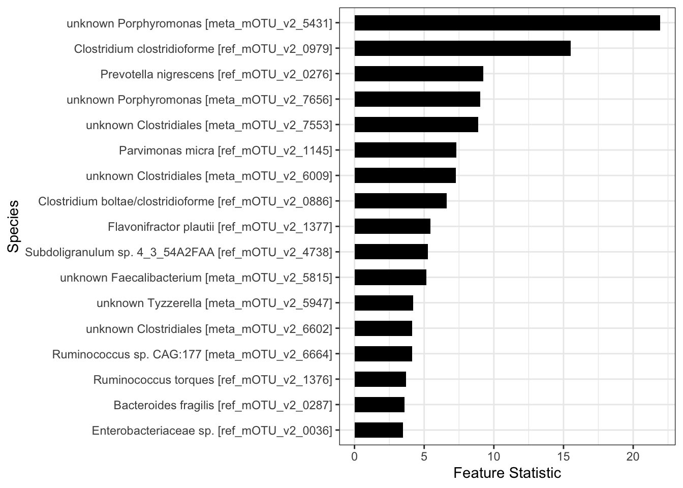
| Version | Author | Date |
|---|---|---|
| ab6400d | Patron | 2024-06-18 |
sessionInfo()R version 4.1.3 (2022-03-10)
Platform: x86_64-apple-darwin17.0 (64-bit)
Running under: macOS Big Sur/Monterey 10.16
Matrix products: default
BLAS: /Library/Frameworks/R.framework/Versions/4.1/Resources/lib/libRblas.0.dylib
LAPACK: /Library/Frameworks/R.framework/Versions/4.1/Resources/lib/libRlapack.dylib
locale:
[1] en_US.UTF-8/en_US.UTF-8/en_US.UTF-8/C/en_US.UTF-8/en_US.UTF-8
attached base packages:
[1] stats graphics grDevices utils datasets methods base
other attached packages:
[1] rstan_2.21.8 StanHeaders_2.21.0-7 ggplot2_3.4.2
[4] knockoff_0.3.6 reshape2_1.4.4 zinck_0.0.0.9000
[7] randomForest_4.7-1.1 workflowr_1.7.1
loaded via a namespace (and not attached):
[1] Rcpp_1.0.10 lattice_0.21-8 prettyunits_1.1.1 getPass_0.2-2
[5] ps_1.7.5 glmnet_4.1-7 rprojroot_2.0.3 digest_0.6.31
[9] foreach_1.5.2 utf8_1.2.3 R6_2.5.1 plyr_1.8.8
[13] stats4_4.1.3 evaluate_0.21 highr_0.10 httr_1.4.6
[17] pillar_1.9.0 rlang_1.1.1 rstudioapi_0.14 whisker_0.4.1
[21] callr_3.7.3 jquerylib_0.1.4 Matrix_1.5-1 rmarkdown_2.22
[25] labeling_0.4.2 splines_4.1.3 stringr_1.5.0 loo_2.6.0
[29] munsell_0.5.0 compiler_4.1.3 httpuv_1.6.11 xfun_0.39
[33] pkgconfig_2.0.3 pkgbuild_1.4.2 shape_1.4.6 htmltools_0.5.5
[37] tidyselect_1.2.0 gridExtra_2.3 tibble_3.2.1 matrixStats_0.63.0
[41] codetools_0.2-19 fansi_1.0.4 withr_2.5.0 crayon_1.5.2
[45] dplyr_1.1.2 later_1.3.1 grid_4.1.3 DBI_1.1.3
[49] jsonlite_1.8.5 gtable_0.3.3 lifecycle_1.0.3 git2r_0.32.0
[53] magrittr_2.0.3 scales_1.2.1 RcppParallel_5.1.7 cli_3.6.1
[57] stringi_1.7.12 cachem_1.0.8 farver_2.1.1 fs_1.6.2
[61] promises_1.2.0.1 bslib_0.5.0 generics_0.1.3 vctrs_0.6.5
[65] iterators_1.0.14 tools_4.1.3 glue_1.6.2 parallel_4.1.3
[69] processx_3.8.1 fastmap_1.1.1 survival_3.5-5 yaml_2.3.7
[73] inline_0.3.19 colorspace_2.1-0 knitr_1.43 sass_0.4.6