Inflammatory Bowel Disease (IBD) Study
Soham Ghosh
2024-06-18
Last updated: 2024-06-18
Checks: 6 1
Knit directory: zinck-website/
This reproducible R Markdown analysis was created with workflowr (version 1.7.1). The Checks tab describes the reproducibility checks that were applied when the results were created. The Past versions tab lists the development history.
The R Markdown is untracked by Git. To know which version of the R
Markdown file created these results, you’ll want to first commit it to
the Git repo. If you’re still working on the analysis, you can ignore
this warning. When you’re finished, you can run
wflow_publish to commit the R Markdown file and build the
HTML.
Great job! The global environment was empty. Objects defined in the global environment can affect the analysis in your R Markdown file in unknown ways. For reproduciblity it’s best to always run the code in an empty environment.
The command set.seed(20240617) was run prior to running
the code in the R Markdown file. Setting a seed ensures that any results
that rely on randomness, e.g. subsampling or permutations, are
reproducible.
Great job! Recording the operating system, R version, and package versions is critical for reproducibility.
Nice! There were no cached chunks for this analysis, so you can be confident that you successfully produced the results during this run.
Great job! Using relative paths to the files within your workflowr project makes it easier to run your code on other machines.
Great! You are using Git for version control. Tracking code development and connecting the code version to the results is critical for reproducibility.
The results in this page were generated with repository version 6e66a4e. See the Past versions tab to see a history of the changes made to the R Markdown and HTML files.
Note that you need to be careful to ensure that all relevant files for
the analysis have been committed to Git prior to generating the results
(you can use wflow_publish or
wflow_git_commit). workflowr only checks the R Markdown
file, but you know if there are other scripts or data files that it
depends on. Below is the status of the Git repository when the results
were generated:
Untracked files:
    Untracked:  analysis/CRC.Rmd
    Untracked:  analysis/Heatmaps.Rmd
    Untracked:  analysis/IBD.Rmd
    Untracked:  analysis/simulation.Rmd

Unstaged changes:
    Modified:   analysis/index.Rmd
Note that any generated files, e.g. HTML, png, CSS, etc., are not included in this status report because it is ok for generated content to have uncommitted changes.
There are no past versions. Publish this analysis with
wflow_publish() to start tracking its development.
IBD Data Analysis
Out of the ten uniformly processed 16S rRNA gene sequencing studies of the IBD mucosal/stool microbiome (https://github.com/biobakery/ibd_paper/tree/paper_publication), we focus on five studies – RISK (430 cases, 201 controls), CS PRISM (359 cases, 38 controls), HMP2 (59 cases, 22 controls), Pouchitis (308 cases, 45 controls), and Mucosal IBD (36 cases, 47 controls). Here cases indicate patients with Ulcerative Colitis (UC) or Crohn’s Disease (CD). We included all \(249\) IBD genera in our analyses.
library(zinck)
library(reshape2)
library(knockoff)
library(ggplot2)
library(rstan)
Loading required package: StanHeadersrstan (Version 2.21.8, GitRev: 2e1f913d3ca3)For execution on a local, multicore CPU with excess RAM we recommend calling
options(mc.cores = parallel::detectCores()).
To avoid recompilation of unchanged Stan programs, we recommend calling
rstan_options(auto_write = TRUE)library(phyloseq)
################################################################################
###################### IBD data genus level ####################################
load("/Users/Patron/Documents/zinLDA research/genera.RData") ## Loading the meta IBD studies
combined_studies <- as.data.frame(t(physeq_genera@otu_table))
study_names <- physeq_genera@sam_data[["dataset_name"]]
#### Study : RISK ####
risk_indices <- which(study_names == "RISK")
risk_otu <- combined_studies[risk_indices, ]
IBD_resp <- physeq_genera@sam_data[["disease"]][risk_indices]
risk_Y <- ifelse(IBD_resp %in% c("CD", "UC"), 1, 0) ## Labelling "CD" or "UC" as 1, rest as 0
#### Study : CS-PRISM ####
prism_indices <- which(study_names == "CS-PRISM")
prism_otu <- combined_studies[prism_indices, ]
IBD_resp <- physeq_genera@sam_data[["disease"]][prism_indices]
prism_Y <- ifelse(IBD_resp %in% c("CD", "UC"), 1, 0)
#### Study : HMP2 ######
hmp_indices <- which(study_names == "HMP2")
hmp_otu <- combined_studies[hmp_indices, ]
IBD_resp <- physeq_genera@sam_data[["disease"]][hmp_indices]
hmp_Y <- ifelse(IBD_resp %in% c("CD", "UC"), 1, 0)
##### Study : MucosalIBD #####
mi_indices <- which(study_names == "MucosalIBD")
mi_otu <- combined_studies[mi_indices, ]
IBD_resp <- physeq_genera@sam_data[["disease"]][mi_indices]
mi_Y <- ifelse(IBD_resp %in% c("CD", "UC"), 1, 0)
##### Study : Pouchitis #####
pouchitis_indices <- which(study_names == "Pouchitis")
pouchitis_otu <- combined_studies[pouchitis_indices, ]
IBD_resp <- physeq_genera@sam_data[["disease"]][pouchitis_indices]
pouchitis_Y <- ifelse(IBD_resp %in% c("CD", "UC"), 1, 0)
######### Combining all the 5 studies together #############
X <- rbind(risk_otu,prism_otu,hmp_otu,mi_otu,pouchitis_otu)
Y <- c(risk_Y,prism_Y,hmp_Y,mi_Y,pouchitis_Y)We train the zinck model on \(X\) with the optimal number of clusters (27), and use the posterior estimates of the latent parameters to generate the knockoff matrix.
zinck_code <- "data {
  int<lower=1> K; // num topics
  int<lower=1> V; // num words
  int<lower=0> D; // num docs
  int<lower=0> n[D, V]; // word counts for each doc

  // hyperparameters
  vector<lower=0, upper=1>[V] delta;
}

parameters {
  simplex[K] theta[D]; // topic mixtures
  vector<lower=0, upper=1>[V] zeta[K]; // zero-inflated betas
  vector<lower=0>[V] gamma1[K];
  vector<lower=0>[V] gamma2[K];
  vector<lower=0>[K] alpha;
}

transformed parameters {
  vector[V] beta[K];

  // Efficiently compute beta using vectorized operations
  for (k in 1:K) {
    vector[V] cum_log1m;
    cum_log1m[1:(V - 1)] = cumulative_sum(log1m(zeta[k, 1:(V - 1)]));
    cum_log1m[V] = 0;
    beta[k] = zeta[k] .* exp(cum_log1m);
    beta[k] = beta[k] / sum(beta[k]);
  }
}


model {
  for (k in 1:K) {
    alpha[k] ~ gamma(100,100);  // Change these hyperparameters as needed
  }
  for (d in 1:D) {
    theta[d] ~ dirichlet(alpha);
  }
  for (k in 1:K) {
    for (m in 1:V) {
        gamma1[k,m] ~ gamma(1,1);
        gamma2[k,m] ~ gamma(1,1);
    }
  }

  // Zero-inflated beta likelihood and data likelihood
  for (k in 1:K) {
    for (m in 1:V) {
      real lp_non_zero = bernoulli_lpmf(0 | delta[m]) + beta_lpdf(zeta[k, m] | gamma1[k, m], gamma2[k, m]);
      real lp_zero = bernoulli_lpmf(1 | delta[m]);
      target += log_sum_exp(lp_non_zero, lp_zero);
    }
  }

  // Compute the eta values and data likelihood more efficiently
  for (d in 1:D) {
    vector[V] eta = theta[d, 1] * beta[1];
    for (k in 2:K) {
      eta += theta[d, k] * beta[k];
    }
    eta = eta / sum(eta);
    n[d] ~ multinomial(eta);
  }
}
"

stan.model = stan_model(model_code = zinck_code)
Trying to compile a simple C fileRunning /Library/Frameworks/R.framework/Resources/bin/R CMD SHLIB foo.c
clang -mmacosx-version-min=10.13 -I"/Library/Frameworks/R.framework/Resources/include" -DNDEBUG -I"/Library/Frameworks/R.framework/Versions/4.1/Resources/library/Rcpp/include/" -I"/Library/Frameworks/R.framework/Versions/4.1/Resources/library/RcppEigen/include/" -I"/Library/Frameworks/R.framework/Versions/4.1/Resources/library/RcppEigen/include/unsupported" -I"/Library/Frameworks/R.framework/Versions/4.1/Resources/library/BH/include" -I"/Library/Frameworks/R.framework/Versions/4.1/Resources/library/StanHeaders/include/src/" -I"/Library/Frameworks/R.framework/Versions/4.1/Resources/library/StanHeaders/include/" -I"/Library/Frameworks/R.framework/Versions/4.1/Resources/library/RcppParallel/include/" -I"/Library/Frameworks/R.framework/Versions/4.1/Resources/library/rstan/include" -DEIGEN_NO_DEBUG -DBOOST_DISABLE_ASSERTS -DBOOST_PENDING_INTEGER_LOG2_HPP -DSTAN_THREADS -DBOOST_NO_AUTO_PTR -include '/Library/Frameworks/R.framework/Versions/4.1/Resources/library/StanHeaders/include/stan/math/prim/mat/fun/Eigen.hpp' -D_REENTRANT -DRCPP_PARALLEL_USE_TBB=1 -I/usr/local/include -fPIC -Wall -g -O2 -c foo.c -o foo.o
In file included from <built-in>:1:
In file included from /Library/Frameworks/R.framework/Versions/4.1/Resources/library/StanHeaders/include/stan/math/prim/mat/fun/Eigen.hpp:13:
In file included from /Library/Frameworks/R.framework/Versions/4.1/Resources/library/RcppEigen/include/Eigen/Dense:1:
In file included from /Library/Frameworks/R.framework/Versions/4.1/Resources/library/RcppEigen/include/Eigen/Core:88:
/Library/Frameworks/R.framework/Versions/4.1/Resources/library/RcppEigen/include/Eigen/src/Core/util/Macros.h:628:1: error: unknown type name 'namespace'
namespace Eigen {
^
/Library/Frameworks/R.framework/Versions/4.1/Resources/library/RcppEigen/include/Eigen/src/Core/util/Macros.h:628:16: error: expected ';' after top level declarator
namespace Eigen {
^
;
In file included from <built-in>:1:
In file included from /Library/Frameworks/R.framework/Versions/4.1/Resources/library/StanHeaders/include/stan/math/prim/mat/fun/Eigen.hpp:13:
In file included from /Library/Frameworks/R.framework/Versions/4.1/Resources/library/RcppEigen/include/Eigen/Dense:1:
/Library/Frameworks/R.framework/Versions/4.1/Resources/library/RcppEigen/include/Eigen/Core:96:10: fatal error: 'complex' file not found
#include <complex>
^~~~~~~~~
3 errors generated.
make: *** [foo.o] Error 1X <- X[,order(decreasing=T,colSums(X,na.rm=T),apply(X,2L,paste,collapse=''))] ## ordering the columns w/ decreasing abundance
dlt <- rep(0,ncol(X)) ## Initializing the deltas with the sparsity of each column
for(t in (1:ncol(X)))
{
dlt[t] <- 1-mean(X[,t]>0)
if(dlt[t]==0)
{
dlt[t] = dlt[t]+0.01
}
if (dlt[t]==1)
{
dlt[t] = dlt[t]-0.01
}
}
zinLDA_stan_data <- list(
K = 27,
V = ncol(X),
D = nrow(X),
n = X,
delta = dlt
)
## Fitting the zinck model ##
set.seed(1)
fitIBD <- vb(stan.model, data=zinLDA_stan_data, algorithm="meanfield", importance_resampling=TRUE, iter=10000,tol_rel_obj=0.01,elbo_samples=500)Chain 1: ------------------------------------------------------------
Chain 1: EXPERIMENTAL ALGORITHM:
Chain 1: This procedure has not been thoroughly tested and may be unstable
Chain 1: or buggy. The interface is subject to change.
Chain 1: ------------------------------------------------------------
Chain 1:
Chain 1:
Chain 1:
Chain 1: Gradient evaluation took 0.7248 seconds
Chain 1: 1000 transitions using 10 leapfrog steps per transition would take 7248 seconds.
Chain 1: Adjust your expectations accordingly!
Chain 1:
Chain 1:
Chain 1: Begin eta adaptation.
Chain 1: Iteration: 1 / 250 [ 0%] (Adaptation)
Chain 1: Iteration: 50 / 250 [ 20%] (Adaptation)
Chain 1: Iteration: 100 / 250 [ 40%] (Adaptation)
Chain 1: Iteration: 150 / 250 [ 60%] (Adaptation)
Chain 1: Iteration: 200 / 250 [ 80%] (Adaptation)
Chain 1: Iteration: 250 / 250 [100%] (Adaptation)
Chain 1: Success! Found best value [eta = 0.1].
Chain 1:
Chain 1: Begin stochastic gradient ascent.
Chain 1: iter ELBO delta_ELBO_mean delta_ELBO_med notes
Chain 1: 100 -126700447.982 1.000 1.000
Chain 1: 200 -77685031.927 0.815 1.000
Chain 1: 300 -59307492.121 0.647 0.631
Chain 1: 400 -50860990.107 0.527 0.631
Chain 1: 500 -45537078.584 0.445 0.310
Chain 1: 600 -41685839.741 0.386 0.310
Chain 1: 700 -38580134.819 0.342 0.166
Chain 1: 800 -36053383.596 0.308 0.166
Chain 1: 900 -33979738.726 0.281 0.117
Chain 1: 1000 -32254605.026 0.258 0.117
Chain 1: 1100 -30792620.765 0.163 0.092
Chain 1: 1200 -29559706.949 0.104 0.081
Chain 1: 1300 -28474935.327 0.077 0.070
Chain 1: 1400 -27530699.160 0.064 0.061
Chain 1: 1500 -26698219.449 0.055 0.053
Chain 1: 1600 -25944401.570 0.049 0.047
Chain 1: 1700 -25287308.192 0.043 0.042
Chain 1: 1800 -24690624.955 0.039 0.038
Chain 1: 1900 -24160947.818 0.035 0.034
Chain 1: 2000 -23683162.157 0.031 0.031
Chain 1: 2100 -23249587.266 0.029 0.029
Chain 1: 2200 -22863841.826 0.026 0.026
Chain 1: 2300 -22511759.353 0.024 0.024
Chain 1: 2400 -22195116.004 0.022 0.022
Chain 1: 2500 -21911818.977 0.020 0.020
Chain 1: 2600 -21658464.199 0.018 0.019
Chain 1: 2700 -21427457.111 0.017 0.017
Chain 1: 2800 -21217341.358 0.015 0.016
Chain 1: 2900 -21028919.131 0.014 0.014
Chain 1: 3000 -20858398.183 0.013 0.013
Chain 1: 3100 -20704895.615 0.012 0.012
Chain 1: 3200 -20558554.504 0.011 0.011
Chain 1: 3300 -20420888.342 0.010 0.010 MEAN ELBO CONVERGED MEDIAN ELBO CONVERGED
Chain 1:
Chain 1: Drawing a sample of size 1000 from the approximate posterior...
Chain 1: COMPLETED.Warning: Pareto k diagnostic value is Inf. Resampling is disabled. Decreasing
tol_rel_obj may help if variational algorithm has terminated prematurely.
Otherwise consider using sampling instead.theta <- fitIBD@sim[["est"]][["theta"]]
beta <- fitIBD@sim[["est"]][["beta"]]
X_tilde <- zinck::generateKnockoff(X,theta,beta,seed=1) ## Generating the kncokoff copyFitting the Random Forest model associating the augmented set of covariates with the outcome of interest, we extract the Feature Importance scores.
set.seed(5)
W <- stat.random_forest(X,X_tilde,Y)
T <- knockoff.threshold(W,fdr=0.1,offset = 0) ## This is the knockoff filter threshold
print(which(W>=T))
[1] 8 16 22 24 28 32 37 61 65 69names <- colnames(X[,which(W>=T)]) ## Extracting the names of the important genera
data.genus <- data.frame(
impscores = sort(W[which(W>=T)], decreasing=FALSE) ,
name = factor(names, levels = names),
y = seq(length(names)) * 0.9
)
plt.genus <- ggplot(data.genus) +
geom_col(aes(impscores, name), fill = "black", width = 0.6)+theme_bw()+ylab("Genera")+xlab("Feature Statistic")
plt.genus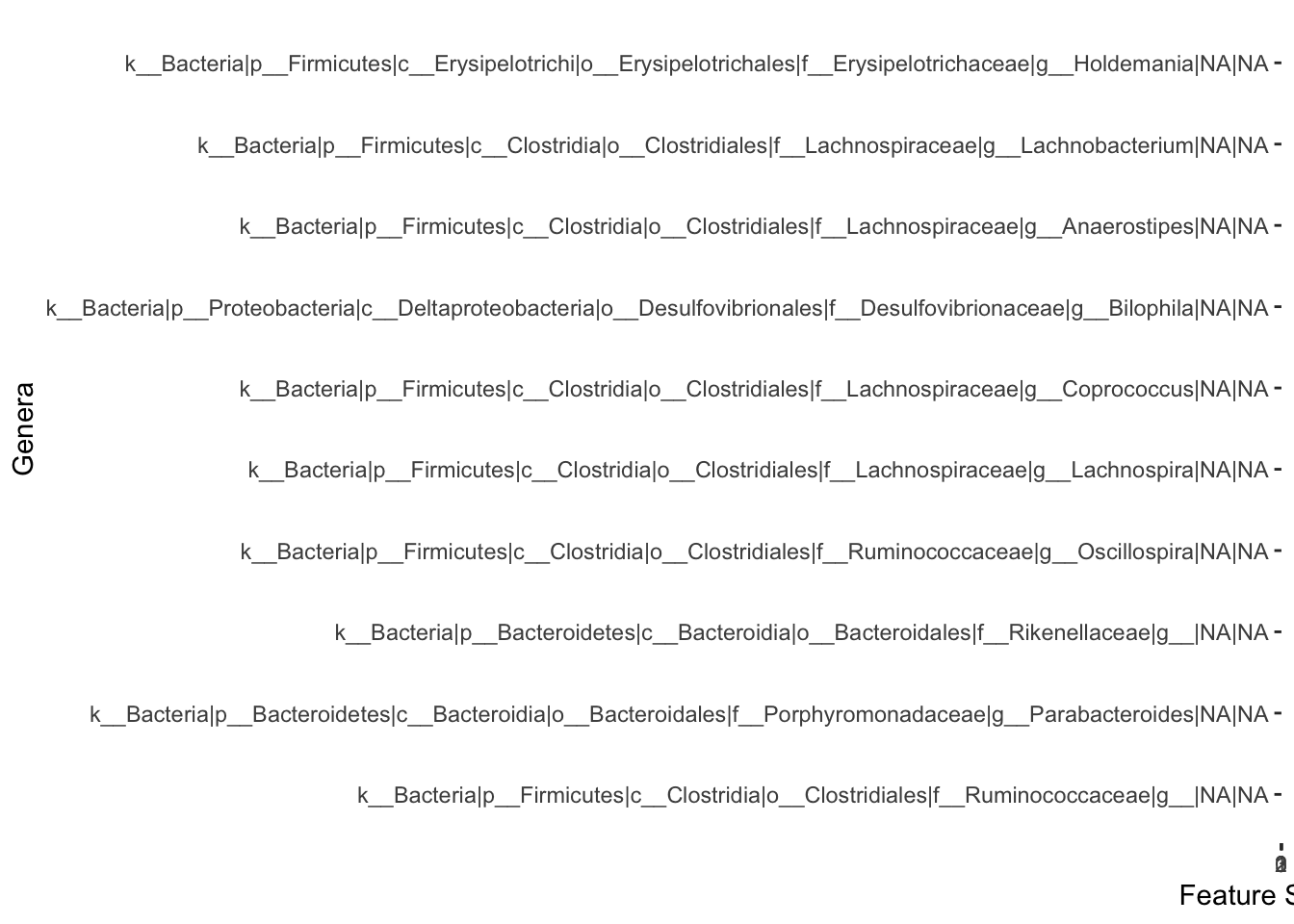
sessionInfo()R version 4.1.3 (2022-03-10)
Platform: x86_64-apple-darwin17.0 (64-bit)
Running under: macOS Big Sur/Monterey 10.16
Matrix products: default
BLAS: /Library/Frameworks/R.framework/Versions/4.1/Resources/lib/libRblas.0.dylib
LAPACK: /Library/Frameworks/R.framework/Versions/4.1/Resources/lib/libRlapack.dylib
locale:
[1] en_US.UTF-8/en_US.UTF-8/en_US.UTF-8/C/en_US.UTF-8/en_US.UTF-8
attached base packages:
[1] stats graphics grDevices utils datasets methods base
other attached packages:
[1] phyloseq_1.38.0 rstan_2.21.8 StanHeaders_2.21.0-7
[4] ggplot2_3.4.2 knockoff_0.3.6 reshape2_1.4.4
[7] zinck_0.0.0.9000 workflowr_1.7.1
loaded via a namespace (and not attached):
[1] nlme_3.1-162 bitops_1.0-7 matrixStats_0.63.0
[4] fs_1.6.2 httr_1.4.6 rprojroot_2.0.3
[7] GenomeInfoDb_1.30.1 tools_4.1.3 bslib_0.5.0
[10] vegan_2.6-4 utf8_1.2.3 R6_2.5.1
[13] mgcv_1.8-42 DBI_1.1.3 BiocGenerics_0.40.0
[16] colorspace_2.1-0 permute_0.9-7 rhdf5filters_1.6.0
[19] ade4_1.7-22 withr_2.5.0 tidyselect_1.2.0
[22] gridExtra_2.3 prettyunits_1.1.1 processx_3.8.1
[25] compiler_4.1.3 git2r_0.32.0 glmnet_4.1-7
[28] cli_3.6.1 Biobase_2.54.0 labeling_0.4.2
[31] sass_0.4.6 scales_1.2.1 randomForest_4.7-1.1
[34] callr_3.7.3 stringr_1.5.0 digest_0.6.31
[37] rmarkdown_2.22 XVector_0.34.0 pkgconfig_2.0.3
[40] htmltools_0.5.5 highr_0.10 fastmap_1.1.1
[43] rlang_1.1.1 rstudioapi_0.14 farver_2.1.1
[46] shape_1.4.6 jquerylib_0.1.4 generics_0.1.3
[49] jsonlite_1.8.5 dplyr_1.1.2 inline_0.3.19
[52] RCurl_1.98-1.12 magrittr_2.0.3 GenomeInfoDbData_1.2.7
[55] loo_2.6.0 biomformat_1.22.0 Matrix_1.5-1
[58] Rhdf5lib_1.16.0 Rcpp_1.0.10 munsell_0.5.0
[61] S4Vectors_0.32.4 fansi_1.0.4 ape_5.7-1
[64] lifecycle_1.0.3 stringi_1.7.12 whisker_0.4.1
[67] yaml_2.3.7 MASS_7.3-60 zlibbioc_1.40.0
[70] rhdf5_2.38.1 pkgbuild_1.4.2 plyr_1.8.8
[73] grid_4.1.3 parallel_4.1.3 promises_1.2.0.1
[76] crayon_1.5.2 lattice_0.21-8 Biostrings_2.62.0
[79] splines_4.1.3 multtest_2.50.0 knitr_1.43
[82] ps_1.7.5 pillar_1.9.0 ranger_0.15.1
[85] igraph_1.4.2 codetools_0.2-19 stats4_4.1.3
[88] glue_1.6.2 evaluate_0.21 getPass_0.2-2
[91] data.table_1.14.8 RcppParallel_5.1.7 vctrs_0.6.5
[94] httpuv_1.6.11 foreach_1.5.2 gtable_0.3.3
[97] cachem_1.0.8 xfun_0.39 later_1.3.1
[100] survival_3.5-5 tibble_3.2.1 iterators_1.0.14
[103] IRanges_2.28.0 cluster_2.1.4