Extracting data from text and geocoding
1 Introduction
In this section, we are going to explore officer-involved shootings (OIS) in Philadelphia. The Philadelphia Police Department posts a lot of information about officer-involved shootings online going back to 2007. Have a look at their OIS webpage. While a lot of information has been posted to the webpage, more information is buried in text and pdf files linked to each of the incidents. In order for us to explore these data, we are going to scrape the basic information from the webpage, have R dig into the text and pdf files for dates, clean up addresses using regular expressions, geocode the addresses to latitude/longitude with the ArcGIS geocoder (using JSON), and then make maps describing the shootings.
Start by loading the packages we’ll need.
library(lubridate)
library(pdftools)
library(jsonlite)
library(sf)
library(leaflet)
library(dplyr)
library(tidyr)
2 Scraping the OIS data
Let’s start by grabbing the raw HTML from the PPD OIS webpage. The website dynamically generates the tables. If we use scan() to pull all the HTML, it will just pull in the HTML code that instructs the web browser to pull in the data to build the tables. That is, the actual data will not be there, but HTML code for the browser to build the tables. To work around this, simply navigate your web browser to https://www.phillypolice.com/ois/. Right-click on the page and select “Save As” and save the HTML page to a convenient data folder on your computer (Save or Save As on some browsers might be elsewhere, like under a File menu). Now that we have let the browser pull all the data to create the tables, we can use scan() to read in the file.
a <- scan(file="10_shapefiles_and_data/Officer Involved Shootings _ Philadelphia Police Department.html",
          what="",sep="\n")
scan() is a very simple function that just pulls in text from a file or URL. It does not attempt to do any formatting. what="" tells scan() to treat what it is reading in as text and sep="\n" tells scan() to break the text apart whenever it encounters a line feed character.
The first several elements of a are just HTML code setting up the page.
a[1:4][1] "<!DOCTYPE html>"
[2] "<!-- saved from url=(0033)https://www.phillypolice.com/ois/ -->"
[3] "<html lang=\"en\"><head><meta http-equiv=\"Content-Type\" content=\"text/html; charset=UTF-8\">"
[4] " " But further on down you will find HTML code containing the OIS information that we seek. Let’s look at one of the 2024 incidents.
i <- grep(">24-22", a)
a[i + 0:9]
[1] " <a class=\"text-primary bold underline cursor-pointer\" :href=\"o.summary\" x-text=\"o.title\" href=\"https://ois.sites.phillypolice.com/ps24-22/\" contenteditable=\"false\" style=\"cursor: pointer;\">24-22</a>"
[2] " </th>"
[3] " <td x-text=\"o.location\">6100 block of West Columbia Avenue</td>"
[4] " <td x-text=\"o.year\">2024</td>"
[5] " <td x-text=\"o.offenderInjury\">N/A</td>"
[6] " <td x-text=\"o.offenderArrested\">N/A</td>"
[7] " <td x-text=\"o.officerInjury\">No</td>"
[8] " <td x-text=\"o.daAction\">Pending</td>"
[9] " <td x-text=\"o.useOfForce\">Pending</td>"
[10] " </tr><tr class=\"text-xs\">" I noticed that for each table row related to an OIS there was some HTML code like x-text="o.title". The same row includes a URL linking to another page with more detailed information. The third line of HTML code contains the address where the shooting occurred. There are additional table cells indicating injuries and how the shooting was adjudicated, but we will not work with these in this exercise.
If we want to get the address for the OIS, we know that it is in a[i+2], two rows after the one with the x-text="o.title" HTML code.
a[i+2][1] " <td x-text=\"o.location\">6100 block of West Columbia Avenue</td>"We just need to strip away the HTML tags and any leading spaces.
gsub("<[^>]*>|^ *", "", a[i+2])[1] "6100 block of West Columbia Avenue"We’ll use a similar strategy for all the shootings and all the data elements we wish to extract. Start by using grep() to find all of the lines of HTML code that start off a row for an OIS from 2013-2024. The data for OISs before 2013 look a little different and involve a little more customization. We’ll just focus on those after 2013. Let’s get the OIS ID, location, year, and the URL for the detailed information for each OIS. The exact date is not shown on the main page, but it is on the incident details page. We will fill in the date later. For now, we will set date=NA for all of the OISs.
i <- grep("o\\.title", a)
ois <- data.frame(id=gsub("<[^>]*>|^ *","",a[i]),
                  date=NA,  # will fill in later
                  location=gsub("<[^>]*>|^ *","",a[i+2]),
                  year    =as.numeric(gsub("<[^>]*>","",a[i+3])),
                  url     =gsub('.* href="([^"]*)".*',"\\1",a[i]))
ois <- ois |>
  filter(year >= 2013)
Everything from the PPD OIS page is now neatly stored in an R data frame.
head(ois) id date location year
1 24-22 NA 6100 block of West Columbia Avenue 2024
2 24-21 NA 3500 block of F Street 2024
3 24-20 NA 2700 block of North 6th Street 2024
4 24-18 NA 1500 block of North 57th Street 2024
5 24-17 NA 2100 block of East Westmoreland Street 2024
6 24-15 NA 1600 South Dover Street 2024
url
1 https://ois.sites.phillypolice.com/ps24-22/
2 https://ois.sites.phillypolice.com/ps24-21/
3 https://ois.sites.phillypolice.com/ps24-20/
4 https://ois.sites.phillypolice.com/ps24-18/
5 https://ois.sites.phillypolice.com/ps24-17/
6 https://ois.sites.phillypolice.com/ps24-15/Now let’s dig into the details of the incident, starting with the first OIS. The hyperlink in the very first OIS incident points to the page https://ois.sites.phillypolice.com/ps24-22/. Let’s read in the text from that page. If you study the HTML code for this page you will see that the detailed description of the incident begins after the line with the word “clearfix” and ends the line before the one with “.entry-content”. We can use grep() to find the line numbers for these two lines and then extract the text between them. We will also use gsub() to remove the HTML tags.
a <- scan(ois$url[1], what="", sep="\n")
iStart <- grep("clearfix", a)       + 1
iEnd <- grep("\\.entry-content", a) - 1
a <- paste(a[iStart:iEnd], collapse="\n")
a <- gsub("<[^>]*>", "", a)
cat(a)
6100 block of West Columbia Avenue
A Philadelphia police officer shot and killed a charging pit bull dog on June 24, 2024 in West Philadelphia.
The officer and his partner were on patrol around 1:43 p.m. when they responded to a radio call for a vicious dog on the 6100 block of West Colombia Avenue.
When officers arrived at the location, an individual flagged down the officers and pointed them toward the aggressive animal. As one officer approached the sidewalk, a black Pit Bull charged at him and the officer discharged his service weapon multiple times, striking the dog. The animal fled to the rear of a property and was later found deceased.
A search for the dog’s owner is ongoing.
The discharging officer is 39 years old, a six-year veteran of the Philadelphia Police Department, and is assigned to the 19th Police District. He has been placed on administrative duty pending the outcome of the Internal Affairs and Officer-Involved Shooting Investigations.
Reading the details here you learn that the date of the incident was June 24, 2024 and you learn that it was shooting of a pit bull that charged at an officer. We will extract the date from this text later.
Let’s also remove spaces, tabs, line feeds at the beginning and end of the text. I’m going to test out my regular expression on some sample text first. I’ve loaded this text with tabs, spaces, carriage returns, and line feeds at the beginning and end.
gsub("^[[:space:]]*|[[:space:]]*$", "",
     "\t \t text to keep \n\n\r\t  ")
[1] "text to keep"Since we now know how to successfully scrape the detailed description for the first incident, we can wrap what we learned in a for-loop and extract the details for all of the incidents.
ois$text <- NA # create a column to hold the text
for(i in 1:nrow(ois))
{
  # wrap scan() in try() in case the page does not exist
  a <- try( scan(ois$url[i], what="", sep="\n", quiet=TRUE) )

  if(class(a)=="try-error")
  { # some pages will not exist
    cat("Could not access webpage for ",ois$id[i],"\n")
  } else
  {
    iStart <- grep("entry-content clearfix", a) + 1
    iEnd   <- grep("\\.entry-content", a)       - 1

    if(length(iEnd)>0 && length(iStart)>0 && (iEnd-iStart > 1))
    {
      a <- paste(a[iStart:iEnd], collapse="\n")
      a <- gsub("<[^>]*>", "", a)
      a <- gsub("^[[:space:]]*|[[:space:]]*$", "", a)
      ois$text[i] <- a
    } else
    { # some will be missing text completely
      cat("No text for ",ois$id[i],"\n")
    }
  }
}
Warning in file(file, "r"): cannot open URL
'https://ois.sites.phillypolice.com/14-15': HTTP status was '404 Not Found'No text for 20-09
No text for 16-42
No text for 15-02
No text for 15-06
No text for 15-09
No text for 15-10
No text for 15-12
No text for 15-13
No text for 15-16
No text for 15-17
No text for 15-18
No text for 15-22
No text for 15-23
No text for 15-24
No text for 15-26
No text for 15-15
No text for 15-25
No text for 15-28
No text for 15-30
No text for 15-31
No text for 15-32
No text for 15-35
No text for 15-36
No text for 15-37
Error in file(file, "r") :
cannot open the connection to 'https://ois.phillypolice.com/14-15'
Could not access webpage for 14-15
No text for 14-16
No text for 14-19
No text for 14-20
No text for 14-21
No text for 14-22
No text for 14-23
No text for 14-24
No text for 14-28
No text for 14-29
No text for 14-30
No text for 14-32 We see that some of the pages do not exist. We will fix this in a moment once we figure out what went wrong. Let’s check the first few text fields to make sure we have what we think we should have there. We will use substring() to avoid printing out some of the very long text descriptions.
substring(ois$text, 1, 30) [1] "6100 block of West Columbia Av" "3500 block of F Street\nA Phila"
[3] "2700 block of North 6th Street" "1500 block of North 57th Stree"
[5] "2100 block of East Westmorelan" "1600 South Dover Street\nOn Thu"
[7] "3000 block of North 16th Stree" "1500 block of South 58th Stree"
[9] "2200 block of West Oxford Aven" "3900 block of Fairmont Avenue\n"
[11] "Unit block of East Cliveden St" "2100 block of Eastburn Avenue\n"
[13] "1000 block of West Dakota Stre" "6200 block of Haverford Avenue"
[15] "1000 block of North 48th Stree" "300 block of Adams Avenue\nOn "
[17] "2800 block of Mascher Street\nA" "2300 block of Borbeck Avenue\nA"
[19] "3600 block of Sepviva Street\nA" "1800 block of South 29th St.\nO"
[21] "8000 block of North Frankford " "3700 block of Fairmount Street"
[23] "7500 block of Whitaker Ave.\nAt" "1500 block of N. 62nd Street\nO"
[25] "Unit Block of E. Phil Ellena S" "7600 block of Lexington Avenue"
[27] "3100 block of Emerald St.\nOn T" "On Monday, August 14, at appro"
[29] "2300 block of Fawn Street\nOn T" "400 block of West Bringhurst S"
[31] "15xx E. Johnson Street\nOn Frid" "200 block of North 60th Street"
[33] "800 block of North 10th Street" "3300 block of North 10th Stree"
[35] "1300 block of Chancellor Stree" "500 block of East Brinton Stre"
[37] "400 block of South Street\nOn S" "2200 block of West Hunting Par"
[39] "4700 block of Leiper Street\nOn" "4000 block of Lancaster Avenue"
[41] "1700 block of Barbara Street\nO" "2000 block of South Beechwood "
[43] "100 block of West Lehigh Avenu" "4800 block of Keyser Street\nOn"
[45] "1700 Dickinson Street\nOn Wedne" "2700 block of Brown Street\nOn "
[47] "1900 block of South Bancroft S" "5700 block of Overbrook Avenue"
[49] "4100 block of Parkside Avenue " "PHILADELPHIA POLICE OFFICER IN"
[51] "9th Street and Hunting Park Av" "3000 block of North Water Stre"
[53] "300 Glen Echo Road \nOn Monday," "Broad Street and Somerville Av"
[55] "3300 Emerald Street\nPS20-34\nOn" "4700 block of Rorer Street\nOn "
[57] "3500 block of Kyle Road\nOn Mon" "3500 block of Wharton Street\nO"
[59] "1900 block of East Hart Lane\nO" "6100 block of Locust Street\nO"
[61] "5600 block of Greene Street\nOn" "Jasper Street and Hart Lane\nOn"
[63] "7600 Block of Roosevelt Blvd\nO" NA
[65] "1500 block of Bailey Street\nOn" "2500 Block of South 7th Street"
[67] "6th Street and McKean\nOn Tuesd" "4200 block of Clarissa Street\n"
[69] "1400 block of Sharpnack Street" "OIS # 19-04\nOn March 6, 2019,"
[71] "OIS #19-6\nOn March 28, 2019, " "OIS #19-09\nOn Saturday April "
[73] "OIS# 19-11\nOn Thursday, April" "OIS 19-13 \nOn Saturday, May "
[75] "OIS# 19-14 \nOn May 20, 2019, " "OIS# 19-20\nOn 9-02-19, at 10:"
[77] "OIS 19-21\n11/2/19\nOn Saturday" "OIS 19-23\n11/21/19\nOn Novembe"
[79] "OIS# 18-01 \nOn Saturday, Janu" "OIS# 18-02\nOn Monday, January"
[81] "OIS# 18-08\nOn Wednesday, Apri" "OIS # 18-12\nOn Friday, June 8"
[83] "OIS# 18-16\nOn Monday, August " "OIS# 18-17\nOn Thursday, Augus"
[85] "OISI # 18-19\nOn Monday, Augus" "OISI # 18-22\nOn Saturday, Aug"
[87] "OIS # 18-25\nOn Wednesday, Nov" "OIS# 18-26\nOn November 13, 20"
[89] "OIS# 18-27\nOn November 13, 20" "OIS 18-28\nAt approximately 8:"
[91] "OIS# 17-03 (February 15, 2017" "OIS# 17-08 (March 29, 2017)\n"
[93] "OIS# 17-17 (June 8, 2017)\nOn " "OIS# 17-19\nOn Wednesday, July"
[95] "OIS# 17-20 \nOn Thursday, July" "OIS# 17-22 \nOn Monday, August"
[97] "OIS# 17-23 \nOn Friday, August" "OIS# 17-25 \nOn Saturday, Augu"
[99] "OIS# 17-28 \nOn Saturday, Sept" "OIS# 17-30\nOn Saturday, Novem"
[101] "OIS# 17-36\nOn Tuesday, Decemb" "OIS# 17-37\nOn Wednesday, Dece"
[103] "OIS# 17-13 \nOn Friday, May 12" "PS# 16-01\n1/07/16\nOn Thursday"
[105] "PS#16-02\n2/02/16\nOn Tuesday, " "PS#16-07\n3/17/16\nOn Thursday,"
[107] "PS# 16-11\n4/17/16\nOn Sunday, " "PS#16-12\n5/03/16\nOn Tuesday, "
[109] "PS#16-13\n5/04/16\nOn Wednesday" "PS# 16-16\n5/20/16\nOn Friday, "
[111] "PS#16-18\n5/31/16\nOn Tuesday, " "PS#16-19\n5/31/16\nOn Tuesday, "
[113] "PS#16-03\n2/04/16\nOn Thursday," "PS#16-10\n4/09/16\nOn Saturday,"
[115] "PS# 16-26\n9/05/16\nOn Monday, " "PS#16-28\n9/08/16\nOn Thursday,"
[117] "PS#16-29\n9/09/16\nOn Friday, S" "PS#16-30\n9/16/16\nOn Friday, S"
[119] "PS#16-32\n9/28/16\nOn Wednesday" "PS# 16-33\n10/18/16\nOn Tuesday"
[121] "PS# 16-34\n10/19/16\nOn Wednesd" "PS# 16-35\n10/19/16\nOn Saturda"
[123] "PS#16-37\n10/27/16\nOn Thursday" "PS#16-38\n11/2/16\nOn Saturday,"
[125] "PS#16-40\n11/07/16\nOn Monday, " "PS#16-43\n11/25/16\nOn Friday, "
[127] NA NA
[129] NA NA
[131] NA NA
[133] NA NA
[135] NA NA
[137] NA NA
[139] NA NA
[141] NA NA
[143] NA NA
[145] NA NA
[147] NA NA
[149] NA "Download the pdf file"
[151] "Download the pdf file" "Download the pdf file"
[153] "Download the pdf file" "Download the pdf file"
[155] "Download the pdf file" "Download the pdf file"
[157] "Download the pdf file" "Download the pdf file"
[159] NA NA
[161] NA NA
[163] NA NA
[165] NA NA
[167] NA NA
[169] NA NA
[171] "Download the pdf file" "Download the pdf file"
[173] "Download the pdf file" "Download the pdf file"
[175] "Download the pdf file" "Download the pdf file"
[177] "Download the pdf file" "Download the pdf file"
[179] "Download the pdf file" "Download the pdf file"
[181] "Download the pdf file" "Download the pdf file"
[183] "Download the pdf file" "Download the pdf file"
[185] "Download the pdf file" "Download the pdf file"
[187] "Download the pdf file" "Download the pdf file"
[189] "Download the pdf file" "Download the pdf file"
[191] "Download the pdf file" "Download the pdf file"
[193] "Download the pdf file" "Download the pdf file"
[195] "Download the pdf file" "Download the pdf file"
[197] "Download the pdf file" "Download the pdf file"
[199] "Download the pdf file" "Download the pdf file"
[201] "Download the pdf file" "Download the pdf file"
[203] "Download the pdf file" "Download the pdf file"
[205] "Download the pdf file" "Download the pdf file"
[207] "Download the pdf file" "Download the pdf file"
[209] "Download the pdf file" "Download the pdf file"
[211] "Download the pdf file" "Download the pdf file"
[213] "Download the pdf file" "Download the pdf file"
[215] "Download the pdf file" "Download the pdf file"
[217] "Download the pdf file" "Download the pdf file"
[219] "Download the pdf file" "Download the pdf file"
[221] "Download the pdf file" Many look good. Some have NA. And some say “Download the pdf file”. If you visit one of those pages associated with an NA you will see that they are essentially blank. For example, visit the page https://ois.sites.phillypolice.com/20-09/ and you will see that the page is essentially blank. But there is another source in pdf format. Have a look at (https://www.phillypolice.com/assets/crime-maps-stats/officer-involved-shootings/20-09.pdf)[https://www.phillypolice.com/assets/crime-maps-stats/officer-involved-shootings/20-09.pdf]. This pdf file has the incident description. We just need to take the base of the URL, “https://www.phillypolice.com/assets/crime-maps-stats/officer-involved-shootings/” and use paste0() to tack on the incident id and a “.pdf” to get the URL for the pdf file. Similarly, if you try to visit one of the detail pages for an incident with “Download the pdf file” you will see that the page has some broken display of the file, but a live link to a pdf document. Inside those pdf documents are the detailed descriptions that we are looking for.
So let’s test this out.
# start by setting all the ones without text to NA
ois$text[ois$text=="Download the pdf file"] <- NA

# for which incidents do we need to get details from pdf files
i <- which(is.na(ois$text))
# provide the URL to the pdf file
ois$url[i] <- paste0("https://www.phillypolice.com/assets/crime-maps-stats/officer-involved-shootings/",ois$id[i],".pdf")

# test reading the description from the first pdf file
i[1]
a <- pdf_text(ois$url[i[1]])
cat(a)
[1] 64
On Friday, March 13, 2020, at 5:51AM, Homicide Detectives assigned to the U.S. Marshals
Fugitive Task Force, SWAT Officers, and uniformed 15th District Police Officers went to a
property in the 1600 block of Bridge Street to execute a murder Arrest Warrant for Male #1.
After knocking and announcing themselves, with no response, SWAT officers breached the door
and went in. While heading upstairs to the second floor, they began taking gunfire from the
second floor, middle bedroom. The shooters were concealed behind the closed door. While
about three steps from the second floor, Officer #3 (in the third position heading upstairs), was
struck in the left shoulder and forearm. Simultaneously, the Officers #1 and #2 (in positions 1
and 2) continued up the stairs. Officer #2 discharged multiple times, striking the middle bedroom
door. When ordered to come out, occupants of the middle room complied and surrendered. The
wounded Officer was removed from the property and rushed him to Temple University Hospital.
He did not survive.
During the exchange of gunfire, one male was struck in the left hand and upper torso. Another
male at the property, was struck in the right leg. Both were transported to hospitals for treatment.
No further injuries were reported in connection with this incident.
Ten (10) firearms, were recovered from the middle bedroom.
*** Information posted in the original summary reflects a preliminary understanding of what
occurred at the time of the incident. This information is posted shortly after the incident and may
be updated as the investigation leads to new information. The District Attorney’s Office is
provided all the information from the PPD’s investigation prior to their charging decision.Here we used the function pdf_text() from the pdftools package to read in the text from the pdf file. For some reason, incident 15-35 has a particularly odd URL that we can fix now.
ois$url[ois$id=="15-35"] <- "https://www.phillypolice.com/assets/crime-maps-stats/officer-involved-shootings/PS15-35-summary-dj.doc.pdf"Now that we know how to read from pdf files, we can loop through all the incidents with missing text and read in the text from their associated pdf files.
for(i in which(is.na(ois$text)))
{
  a <- pdf_text(ois$url[i])
  # combine multiple pages into one page
  a <- paste(a, collapse="\n")
  a <- gsub("^[[:space:]]*|[[:space:]]*$", "", a)
  ois$text[i] <- a
}

# check incident descriptions
substring(ois$text, 1, 30)
[1] "6100 block of West Columbia Av"
[2] "3500 block of F Street\nA Phila"
[3] "2700 block of North 6th Street"
[4] "1500 block of North 57th Stree"
[5] "2100 block of East Westmorelan"
[6] "1600 South Dover Street\nOn Thu"
[7] "3000 block of North 16th Stree"
[8] "1500 block of South 58th Stree"
[9] "2200 block of West Oxford Aven"
[10] "3900 block of Fairmont Avenue\n"
[11] "Unit block of East Cliveden St"
[12] "2100 block of Eastburn Avenue\n"
[13] "1000 block of West Dakota Stre"
[14] "6200 block of Haverford Avenue"
[15] "1000 block of North 48th Stree"
[16] "300 block of Adams Avenue\nOn "
[17] "2800 block of Mascher Street\nA"
[18] "2300 block of Borbeck Avenue\nA"
[19] "3600 block of Sepviva Street\nA"
[20] "1800 block of South 29th St.\nO"
[21] "8000 block of North Frankford "
[22] "3700 block of Fairmount Street"
[23] "7500 block of Whitaker Ave.\nAt"
[24] "1500 block of N. 62nd Street\nO"
[25] "Unit Block of E. Phil Ellena S"
[26] "7600 block of Lexington Avenue"
[27] "3100 block of Emerald St.\nOn T"
[28] "On Monday, August 14, at appro"
[29] "2300 block of Fawn Street\nOn T"
[30] "400 block of West Bringhurst S"
[31] "15xx E. Johnson Street\nOn Frid"
[32] "200 block of North 60th Street"
[33] "800 block of North 10th Street"
[34] "3300 block of North 10th Stree"
[35] "1300 block of Chancellor Stree"
[36] "500 block of East Brinton Stre"
[37] "400 block of South Street\nOn S"
[38] "2200 block of West Hunting Par"
[39] "4700 block of Leiper Street\nOn"
[40] "4000 block of Lancaster Avenue"
[41] "1700 block of Barbara Street\nO"
[42] "2000 block of South Beechwood "
[43] "100 block of West Lehigh Avenu"
[44] "4800 block of Keyser Street\nOn"
[45] "1700 Dickinson Street\nOn Wedne"
[46] "2700 block of Brown Street\nOn "
[47] "1900 block of South Bancroft S"
[48] "5700 block of Overbrook Avenue"
[49] "4100 block of Parkside Avenue "
[50] "PHILADELPHIA POLICE OFFICER IN"
[51] "9th Street and Hunting Park Av"
[52] "3000 block of North Water Stre"
[53] "300 Glen Echo Road \nOn Monday,"
[54] "Broad Street and Somerville Av"
[55] "3300 Emerald Street\nPS20-34\nOn"
[56] "4700 block of Rorer Street\nOn "
[57] "3500 block of Kyle Road\nOn Mon"
[58] "3500 block of Wharton Street\nO"
[59] "1900 block of East Hart Lane\nO"
[60] "6100 block of Locust Street\nO"
[61] "5600 block of Greene Street\nOn"
[62] "Jasper Street and Hart Lane\nOn"
[63] "7600 Block of Roosevelt Blvd\nO"
[64] "On Friday, March 13, 2020, at "
[65] "1500 block of Bailey Street\nOn"
[66] "2500 Block of South 7th Street"
[67] "6th Street and McKean\nOn Tuesd"
[68] "4200 block of Clarissa Street\n"
[69] "1400 block of Sharpnack Street"
[70] "OIS # 19-04\nOn March 6, 2019,"
[71] "OIS #19-6\nOn March 28, 2019, "
[72] "OIS #19-09\nOn Saturday April "
[73] "OIS# 19-11\nOn Thursday, April"
[74] "OIS 19-13 \nOn Saturday, May "
[75] "OIS# 19-14 \nOn May 20, 2019, "
[76] "OIS# 19-20\nOn 9-02-19, at 10:"
[77] "OIS 19-21\n11/2/19\nOn Saturday"
[78] "OIS 19-23\n11/21/19\nOn Novembe"
[79] "OIS# 18-01 \nOn Saturday, Janu"
[80] "OIS# 18-02\nOn Monday, January"
[81] "OIS# 18-08\nOn Wednesday, Apri"
[82] "OIS # 18-12\nOn Friday, June 8"
[83] "OIS# 18-16\nOn Monday, August "
[84] "OIS# 18-17\nOn Thursday, Augus"
[85] "OISI # 18-19\nOn Monday, Augus"
[86] "OISI # 18-22\nOn Saturday, Aug"
[87] "OIS # 18-25\nOn Wednesday, Nov"
[88] "OIS# 18-26\nOn November 13, 20"
[89] "OIS# 18-27\nOn November 13, 20"
[90] "OIS 18-28\nAt approximately 8:"
[91] "OIS# 17-03 (February 15, 2017"
[92] "OIS# 17-08 (March 29, 2017)\n"
[93] "OIS# 17-17 (June 8, 2017)\nOn "
[94] "OIS# 17-19\nOn Wednesday, July"
[95] "OIS# 17-20 \nOn Thursday, July"
[96] "OIS# 17-22 \nOn Monday, August"
[97] "OIS# 17-23 \nOn Friday, August"
[98] "OIS# 17-25 \nOn Saturday, Augu"
[99] "OIS# 17-28 \nOn Saturday, Sept"
[100] "OIS# 17-30\nOn Saturday, Novem"
[101] "OIS# 17-36\nOn Tuesday, Decemb"
[102] "OIS# 17-37\nOn Wednesday, Dece"
[103] "OIS# 17-13 \nOn Friday, May 12"
[104] "PS# 16-01\n1/07/16\nOn Thursday"
[105] "PS#16-02\n2/02/16\nOn Tuesday, "
[106] "PS#16-07\n3/17/16\nOn Thursday,"
[107] "PS# 16-11\n4/17/16\nOn Sunday, "
[108] "PS#16-12\n5/03/16\nOn Tuesday, "
[109] "PS#16-13\n5/04/16\nOn Wednesday"
[110] "PS# 16-16\n5/20/16\nOn Friday, "
[111] "PS#16-18\n5/31/16\nOn Tuesday, "
[112] "PS#16-19\n5/31/16\nOn Tuesday, "
[113] "PS#16-03\n2/04/16\nOn Thursday,"
[114] "PS#16-10\n4/09/16\nOn Saturday,"
[115] "PS# 16-26\n9/05/16\nOn Monday, "
[116] "PS#16-28\n9/08/16\nOn Thursday,"
[117] "PS#16-29\n9/09/16\nOn Friday, S"
[118] "PS#16-30\n9/16/16\nOn Friday, S"
[119] "PS#16-32\n9/28/16\nOn Wednesday"
[120] "PS# 16-33\n10/18/16\nOn Tuesday"
[121] "PS# 16-34\n10/19/16\nOn Wednesd"
[122] "PS# 16-35\n10/19/16\nOn Saturda"
[123] "PS#16-37\n10/27/16\nOn Thursday"
[124] "PS#16-38\n11/2/16\nOn Saturday,"
[125] "PS#16-40\n11/07/16\nOn Monday, "
[126] "PS#16-43\n11/25/16\nOn Friday, "
[127] "PS# 16-42\n\n11/12/16\n\nOn Saturd"
[128] "PS#15-02\n\n1/08/15\n\nOn Thursday"
[129] "PS#15-06\n\n2/04/15\n\nOn Wednesda"
[130] "PS#15-09\n\n3/05/15\n\nOn Thursday"
[131] "PS#15-10\n\n3/07/15\n\nOn Saturday"
[132] "PS#15-12\n\n3/20/15\n\nOn Friday, "
[133] "PS#15-13\n\n3/24/15\n\nOn Tuesday,"
[134] "PS#15-16\n\n4/22/15\n\nOn Wednesda"
[135] "PS#15-17\n\n4/23/15\n\nOn Thursday"
[136] "PS#15-18\n\n4/24/15\n\nOn Friday, "
[137] "PS#15-22\n\n5/12/15\n\nOn Tuesday,"
[138] "PS#15-23\n\n5/24/15\n\nOn Sunday, "
[139] "PS#15-24\n\n5/30/15\n\nOn Saturday"
[140] "PS#15-26\n\n6/04/15\n\nOn Thursday"
[141] "PS#15-15\n\n4/16/15\n\nOn Thursday"
[142] "PS#15-25\n\n6/03/15\n\nOn Wednesda"
[143] "PS#15-28\n\n6/07/15\n\nOn Sunday, "
[144] "PS#15-30\n\n6/22/15\n\nOn Monday, "
[145] "PS#15-31\n\n7/17/15\n\nOn Friday, "
[146] "PS#15-32\n\n7/22/15\n\nOn Wednesda"
[147] "PS#1535\n\nOn Wednesday, August"
[148] "PS#15-36\n\n8/26/15\n\nOn Wednesda"
[149] "PS#15-37\n\n9/14/15\n\nOn Monday, "
[150] "PS#15-41\n\n11/16/15\n\nOn Monday,"
[151] "PS#14-01\n\n1/11/14\n\nOn Saturday"
[152] "PS#14-02\n\n1/13/14\n\nOn Monday, "
[153] "PS#14-03\n\n1/27/14\n\nOn Monday, "
[154] "PS#14-04\n\n1/30/14\n\nOn Thursday"
[155] "PS#14-06\n\n2/04/14\n\nOn Tuesday,"
[156] "PS# 14-07\n\n2/07/14\n\nOn Friday,"
[157] "PS# 14-11\n\n3/08/14\n\nOn Saturda"
[158] "PS# 14-12\n\n3/25/14\n\nOn Tuesday"
[159] "PS#14-15\n\n04/22/14\n\nOn Tuesday"
[160] "PS#14-16\n\n04/26/14\n\nOn Saturda"
[161] "PS#14-19\n\n05/23/14\n\nOn Friday,"
[162] "PS#14-20\n\n05/26/14\n\nOn Monday,"
[163] "PS# 14-21\n\n6/15/14\n\nOn Sunday,"
[164] "PS# 14-22\n\n6/23/14\n\nOn Monday,"
[165] "PS#14-23\n\n06/25/14\n\nOn Wednesd"
[166] "PS#14-24\n\n07/21/14\n\n\nOn Monday"
[167] "PS#14-28\n\n07/30/14\n\nOn Wednesd"
[168] "PS#14-29\n\n07/30/14\n\nOn Wednesd"
[169] "PS#14-30\n\n08/01/14\n\nOn Friday,"
[170] "PS#14-32\n\n08/19/14\n\nOn Tuesday"
[171] "PS#14-35\n\n08/21/14\n\nOn Friday,"
[172] "PS#14-37\n\n09/08/14\n\nOn Monday,"
[173] "PS#14-40\n\n09/21/14\n\nOn Sunday,"
[174] "PS#14-41\n\n09/30/14\n\nOn Tuesday"
[175] "PS#14-36\n\n09/07/14\n\nOn Sunday,"
[176] "PS#14-44\n\n11/30/14\n\nOn Saturda"
[177] "This summary has been updated."
[178] "PS#14-42\n\n10/29/14\n\nOn Wednesd"
[179] "PS#14-43\n\n11/12/14\n\nOn Wednesd"
[180] "PS# 13-75\n\n12/30/13\n\nOn Monday"
[181] "PS# 13-74\n\n12/30/13\n\t \nOn Mon"
[182] "PS# 13-73\n\n12/26/13\n\nOn Thursd"
[183] "PS# 13-72\n\n12/13/13\n\t \nOn Fri"
[184] "PS# 13-71\n\n11/30/13\n\nOn Saturd"
[185] "PS# 13-70\n\n11/27/13\n\t \nOn Wed"
[186] "PS# 13-67\n\n11/12/13\n\nOn Tuesda"
[187] "PS# 13-65\n\n11/02/13\n\nOn Saturd"
[188] "PS# 13-63\n\n10/25/13\n\nOn Friday"
[189] "PS# 13-57\n\n9/22/13\n\nOn Sunday,"
[190] "PS# 13-54\n\n9/07/13\n\nOn Saturda"
[191] "PS# 13-52\n\n8/30/13\n\nOn Friday,"
[192] "PS# 13-51\n\n8/20/13\n\nOn Tuesday"
[193] "PS# 13-45\n\n7/28/13\n\nOn Sunday,"
[194] "PS# 13-43\n\n07/22/13\n\nOn Monday"
[195] "PS# 13-42\n\n07/22/13\n\nOn Monday"
[196] "PS# 13-41\n\n07/21/13\n\nOn Sunday"
[197] "PS# 13-39\n\n7/17/13\n\nOn 7/17/13"
[198] "PS# 13-37\n\n07/08/13\n\nOn Monday"
[199] "PS# 13-34\n\n5/29/13\n\nOn 5-29-13"
[200] "PS#13-36\n\n06/29/13\n\nOn Saturda"
[201] "PS# 13-33\n\n5/29/13\n\nOn 5/29/13"
[202] "PS# 13-32\n\n5/29/13\n\nOn 5/29/13"
[203] "PS# 13-30\n\n5/25/13\n\nOn 5/25/13"
[204] "PS# 13-29\n\n5/23/13\n\nOn 5/23/13"
[205] "PS# 13-28\n\n5/22/13\n\nOn 5/22/13"
[206] "PS# 13-27\n\n5/22/13\n\nOn 5/22/13"
[207] "PS# 13-24\n\n5/14/13\n\nOn 5/14/13"
[208] "PS# 13-22\n\n5/12/13\n\nOn 5/12/13"
[209] "PS# 13-21\n\n5/9/13\n\nOn 5/9/13, "
[210] "PS# 13-19\n\n5/4/13\n\nOn 5/4/13, "
[211] "PS# 13-17\n\n4/29/13\n\nOn 4/29/13"
[212] "PS# 13-14\n\n4/7/13\n\nOn 4/7/13, "
[213] "PS# 13-13\n\n4/4/13\n\nOn 4/4/13, "
[214] "PS# 13-11\n\n3/28/13\n\nOn 3/28/13"
[215] "PS# 13-10\n\n3/17/13\n\nOn 3/17/13"
[216] "PS# 13-09\n\n3/7/13\n\nOn 3/7/13, "
[217] "PS# 13-08\n\n2/28/13\n\nOn 2/28/13"
[218] "PS# 13-06\n\n02/4/13\n\nOn 2/4/13,"
[219] "PS# 13-05\n\n2/1/13\n\nOn 2/1/13, "
[220] "PS# 13-04\n\n1/17/13\n\nOn 1/17/13"
[221] "PS# 13-02\n\n1/4/13\n\nOn 1/4/13, " 3 Extracting dates from the text
We can see that the incident dates are buried in these incident descriptions. We can extract those dates with regular expressions. The dates may come in a variety of formats, but we can use the lubridate package to parse them. Let’s start
# extract dates in January 11, 2024 format
a <- gsub(".*(January|February|March|April|May|June|July|August|September|October|November|December)( [0-9]{1,2})(, 20[0-9]{2})?.*",
          "\\1\\2\\3", ois$text)
For those incidents matching that January 11, 2024 format, they should have less than 20 characters in them. Let’s check those out.
# which ones we found dates
i <- nchar(a) < 20
a[i]
[1] "June 24, 2024" "June 22, 2024" "June 15"
[4] "June 5, 2024" "May 30, 2024" "May 23, 2024"
[7] "May 15, 2024" "May 14, 2024" "May 14"
[10] "May 1" "April 20, 2024" "April 17, 2024"
[13] "April 15, 2024" "April 14, 2024" "April 10"
[16] "February 15, 2024" "January 26" "January 17, 2024"
[19] "January 10, 2024" "December 31, 2023" "December 10, 2023"
[22] "November 4, 2023" "October 4" "October 4, 2023"
[25] "October 2, 2023" "September 27, 2023" "September 14, 2023"
[28] "August 14" "May 4, 2023" "April 29, 2023"
[31] "March 24, 2023" "February 8, 2023" "August 21, 2022"
[34] "October 7, 2022" "September 11, 2022" "September 10, 2022"
[37] "June 4, 2022" "May 11, 2022" "March 19, 2022"
[40] "March 1, 2022" "February 15, 2022" "February 11, 2022"
[43] "February 9, 2022" "November 20" "January 4, 2022"
[46] "August 18" "July 22, 2021" "June 14, 2021"
[49] "April 7, 2021" "November 30, 2020" "February 20, 2020"
[52] "February 28, 2020" "March 13, 2020" "April 10, 2020"
[55] "May 9, 2020" "June 23, 2020" "August 18, 2020"
[58] "September 18, 2020" "March 6, 2019" "March 28, 2019"
[61] "April 20, 2019" "April 25, 2019" "May 11"
[64] "May 20, 2019" "November 2, 2019" "November 21, 2019"
[67] "January 13" "January 29" "April 18, 2018"
[70] "June 8, 2018" "August 6, 2018" "August 9, 2018"
[73] "August 20, 2018" "August 25, 2018" "November 7, 2018"
[76] "November 13, 2018" "November 13, 2018" "December 5, 2018"
[79] "February 15" "March 29, 2017" "June 8"
[82] "July 19" "July 27, 2017" "August 7, 2017"
[85] "August 11, 2017" "August 19, 2017" "September 23, 2017"
[88] "November 11, 2017" "December 26, 2017" "December 27, 2017"
[91] "May 12, 2017" "January 7, 2016" "February 2, 2016"
[94] "March 17, 2016" "April 17, 2016" "May 3, 2016"
[97] "May 4, 2016" "May 20, 2016" "May 31, 2016"
[100] "May 31, 2016" "February 4, 2016" "April 9, 2016"
[103] "September 5, 2016" "September 8, 2016" "September 9, 2016"
[106] "September 16, 2016" "September 9, 2016" "October 18, 2016"
[109] "October 19, 2016" "October 22, 2016" "October 27, 2016"
[112] "October 29, 2016" "November 7, 2016" "November 25, 2016"
[115] "November 12, 2016" "January 8, 2015" "February 4, 2015"
[118] "March 5, 2015" "March 24, 2015" "April 22, 2015"
[121] "April 23, 2015" "April 24, 2015" "May 12, 2015"
[124] "May 24, 2015" "May 30, 2015" "June 4, 2015"
[127] "April 16, 2015" "June 3, 2015" "June 7, 2015"
[130] "June 22, 2015" "July 17, 2015" "July 22, 2015"
[133] "August 26, 2015" "August 26, 2015" "November 16, 2015"
[136] "April 22, 2014" "May 23, 2014" "May 26, 2014"
[139] "June 15, 2014" "June 23, 2014" "June 25, 2014"
[142] "December 15, 2014" "October 29, 2014" "November 12, 2014" The code seems to work for many dates, but we also see that some of the dates did not include the year. Remember that we scraped the year of the incident and have it stored in ois$year already. For those missing the year, we can simply paste it on the end of those dates.
# which ones have the year included
j <- grepl("20[0-9]{2}", a[i])
# show those dates missing the year
a[i][!j]
[1] "June 15" "May 14" "May 1" "April 10" "January 26"
[6] "October 4" "August 14" "November 20" "August 18" "May 11"
[11] "January 13" "January 29" "February 15" "June 8" "July 19" # paste the year on the end of those dates
a[i][!j] <- paste0(a[i][!j], ", ", ois$year[i][!j])
# check the result
a[i] [1] "June 24, 2024" "June 22, 2024" "June 15, 2024"
[4] "June 5, 2024" "May 30, 2024" "May 23, 2024"
[7] "May 15, 2024" "May 14, 2024" "May 14, 2024"
[10] "May 1, 2024" "April 20, 2024" "April 17, 2024"
[13] "April 15, 2024" "April 14, 2024" "April 10, 2024"
[16] "February 15, 2024" "January 26, 2024" "January 17, 2024"
[19] "January 10, 2024" "December 31, 2023" "December 10, 2023"
[22] "November 4, 2023" "October 4, 2023" "October 4, 2023"
[25] "October 2, 2023" "September 27, 2023" "September 14, 2023"
[28] "August 14, 2023" "May 4, 2023" "April 29, 2023"
[31] "March 24, 2023" "February 8, 2023" "August 21, 2022"
[34] "October 7, 2022" "September 11, 2022" "September 10, 2022"
[37] "June 4, 2022" "May 11, 2022" "March 19, 2022"
[40] "March 1, 2022" "February 15, 2022" "February 11, 2022"
[43] "February 9, 2022" "November 20, 2022" "January 4, 2022"
[46] "August 18, 2021" "July 22, 2021" "June 14, 2021"
[49] "April 7, 2021" "November 30, 2020" "February 20, 2020"
[52] "February 28, 2020" "March 13, 2020" "April 10, 2020"
[55] "May 9, 2020" "June 23, 2020" "August 18, 2020"
[58] "September 18, 2020" "March 6, 2019" "March 28, 2019"
[61] "April 20, 2019" "April 25, 2019" "May 11, 2019"
[64] "May 20, 2019" "November 2, 2019" "November 21, 2019"
[67] "January 13, 2018" "January 29, 2018" "April 18, 2018"
[70] "June 8, 2018" "August 6, 2018" "August 9, 2018"
[73] "August 20, 2018" "August 25, 2018" "November 7, 2018"
[76] "November 13, 2018" "November 13, 2018" "December 5, 2018"
[79] "February 15, 2017" "March 29, 2017" "June 8, 2017"
[82] "July 19, 2017" "July 27, 2017" "August 7, 2017"
[85] "August 11, 2017" "August 19, 2017" "September 23, 2017"
[88] "November 11, 2017" "December 26, 2017" "December 27, 2017"
[91] "May 12, 2017" "January 7, 2016" "February 2, 2016"
[94] "March 17, 2016" "April 17, 2016" "May 3, 2016"
[97] "May 4, 2016" "May 20, 2016" "May 31, 2016"
[100] "May 31, 2016" "February 4, 2016" "April 9, 2016"
[103] "September 5, 2016" "September 8, 2016" "September 9, 2016"
[106] "September 16, 2016" "September 9, 2016" "October 18, 2016"
[109] "October 19, 2016" "October 22, 2016" "October 27, 2016"
[112] "October 29, 2016" "November 7, 2016" "November 25, 2016"
[115] "November 12, 2016" "January 8, 2015" "February 4, 2015"
[118] "March 5, 2015" "March 24, 2015" "April 22, 2015"
[121] "April 23, 2015" "April 24, 2015" "May 12, 2015"
[124] "May 24, 2015" "May 30, 2015" "June 4, 2015"
[127] "April 16, 2015" "June 3, 2015" "June 7, 2015"
[130] "June 22, 2015" "July 17, 2015" "July 22, 2015"
[133] "August 26, 2015" "August 26, 2015" "November 16, 2015"
[136] "April 22, 2014" "May 23, 2014" "May 26, 2014"
[139] "June 15, 2014" "June 23, 2014" "June 25, 2014"
[142] "December 15, 2014" "October 29, 2014" "November 12, 2014" We now have the date for 144 of the incidents. The rest of the dates have formats that are in some variation of 01/11/2024 or 01-11-2024 or 01/11/24 or 01-11-24, sometimes with / separators and sometimes with - separators and sometimes with a four digit year and sometimes with a two digit year. We can craft our regular expression to capture all these variations.
# get the remaining dates in #/#/# or #-#-# format
a[!i] <- gsub(".*[^0-9]([0-9]{1,2}[/-][0-9]{1,2}[/-](20)?[1-2][0-9])[^0-9].*",
     "\\1", a[!i])
Let’s check if all our regular expressions got us legitimate dates.
a [1] "June 24, 2024" "June 22, 2024" "June 15, 2024"
[4] "June 5, 2024" "May 30, 2024" "May 23, 2024"
[7] "May 15, 2024" "May 14, 2024" "May 14, 2024"
[10] "May 1, 2024" "April 20, 2024" "April 17, 2024"
[13] "April 15, 2024" "April 14, 2024" "April 10, 2024"
[16] "February 15, 2024" "January 26, 2024" "January 17, 2024"
[19] "January 10, 2024" "December 31, 2023" "December 10, 2023"
[22] "November 4, 2023" "October 4, 2023" "October 4, 2023"
[25] "October 2, 2023" "September 27, 2023" "September 14, 2023"
[28] "August 14, 2023" "May 4, 2023" "April 29, 2023"
[31] "March 24, 2023" "February 8, 2023" "August 21, 2022"
[34] "October 7, 2022" "September 11, 2022" "September 10, 2022"
[37] "June 4, 2022" "May 11, 2022" "4/7/22"
[40] "March 19, 2022" "March 1, 2022" "February 15, 2022"
[43] "February 11, 2022" "February 9, 2022" "November 20, 2022"
[46] "1-31-2022" "January 4, 2022" "10-26-21"
[49] "10-4-2021" "August 18, 2021" "7-29-21"
[52] "July 22, 2021" "June 14, 2021" "April 7, 2021"
[55] "12-25-2020" "12-9-2020" "November 30, 2020"
[58] "11-27-20" "11-12-20" "10-26-2020"
[61] "10-8-2020" "February 20, 2020" "February 28, 2020"
[64] "March 13, 2020" "April 10, 2020" "May 9, 2020"
[67] "June 23, 2020" "August 18, 2020" "September 18, 2020"
[70] "March 6, 2019" "March 28, 2019" "April 20, 2019"
[73] "April 25, 2019" "May 11, 2019" "May 20, 2019"
[76] "9-02-19" "November 2, 2019" "November 21, 2019"
[79] "January 13, 2018" "January 29, 2018" "April 18, 2018"
[82] "June 8, 2018" "August 6, 2018" "August 9, 2018"
[85] "August 20, 2018" "August 25, 2018" "November 7, 2018"
[88] "November 13, 2018" "November 13, 2018" "December 5, 2018"
[91] "February 15, 2017" "March 29, 2017" "June 8, 2017"
[94] "July 19, 2017" "July 27, 2017" "August 7, 2017"
[97] "August 11, 2017" "August 19, 2017" "September 23, 2017"
[100] "November 11, 2017" "December 26, 2017" "December 27, 2017"
[103] "May 12, 2017" "January 7, 2016" "February 2, 2016"
[106] "March 17, 2016" "April 17, 2016" "May 3, 2016"
[109] "May 4, 2016" "May 20, 2016" "May 31, 2016"
[112] "May 31, 2016" "February 4, 2016" "April 9, 2016"
[115] "September 5, 2016" "September 8, 2016" "September 9, 2016"
[118] "September 16, 2016" "September 9, 2016" "October 18, 2016"
[121] "October 19, 2016" "October 22, 2016" "October 27, 2016"
[124] "October 29, 2016" "November 7, 2016" "November 25, 2016"
[127] "November 12, 2016" "January 8, 2015" "February 4, 2015"
[130] "March 5, 2015" "3/7/15" "3/20/15"
[133] "March 24, 2015" "April 22, 2015" "April 23, 2015"
[136] "April 24, 2015" "May 12, 2015" "May 24, 2015"
[139] "May 30, 2015" "June 4, 2015" "April 16, 2015"
[142] "June 3, 2015" "June 7, 2015" "June 22, 2015"
[145] "July 17, 2015" "July 22, 2015" "August 26, 2015"
[148] "August 26, 2015" "9/14/15" "November 16, 2015"
[151] "1/11/14" "1/13/14" "1/27/14"
[154] "1/30/14" "2/04/14" "2/07/14"
[157] "3/08/14" "3/25/14" "April 22, 2014"
[160] "4/26/14" "May 23, 2014" "May 26, 2014"
[163] "June 15, 2014" "June 23, 2014" "June 25, 2014"
[166] "7/21/14" "7/30/14" "7/30/14"
[169] "8/01/14" "8/19/14" "8/21/14"
[172] "9/08/14" "9/21/14" "9/30/14"
[175] "9/07/14" "11/30/14" "December 15, 2014"
[178] "October 29, 2014" "November 12, 2014" "12/30/13"
[181] "12/30/13" "12/26/13" "12/12/13"
[184] "11/30/13" "11/27/13" "11/12/13"
[187] "11/02/13" "10/25/13" "9/22/13"
[190] "9-07-13" "8-30-13" "8/20/13"
[193] "7/28/13" "7/22/13" "7/22/13"
[196] "7/21/13" "7/17/13" "7/08/13"
[199] "5-29-13" "6/29/13" "5/29/13"
[202] "5/29/13" "5/25/13" "5/23/13"
[205] "5/22/13" "5/22/13" "5/14/13"
[208] "5/12/13" "5/9/13" "5/4/13"
[211] "4/29/13" "4/7/13" "4/4/13"
[214] "3/28/13" "3/17/13" "3/7/13"
[217] "2/28/13" "2/4/13" "2/1/13"
[220] "1/17/13" "1/4/13" They are in all different formats, but they all look like legitimate dates. The mdy() function can standardize them all since they are all in month/day/year format.
ois$date <- mdy(a)For a little check, let’s check if there are any incidents where the year we scraped from the webpage differs from the year we extracted from the incident descriptions.
ois |> filter(year(date) != year) id date location year
1 17-13 2017-05-12 1200 block of south 51st street 2016
url
1 https://ois.phillypolice.com/17-13
text
1 OIS# 17-13 \nOn Friday, May 12, 2017, at approximately 2:42 AM, 12th District uniformed officers responded to a radio call for a male violating a Protection From Abuse (PFA) order inside a residence on the 1200 block of south 51 street. The offender was inside the 2nd floor front bedroom. A female complainant stated the male might be armed with a knife. The male refused officers’ direction to open the door and come out of the room. Officer number one forced the door open, and the offender, armed with a ten-inch knife, moved towards the officers. Officer number two deployed his ECW (Taser), contacting the offender, momentarily causing him to fall onto the bed. The offender stood up and while still holding the knife, moved towards the officers. Officer number one discharged his service weapon, striking the offender in the torso. The offender was transported to Penn Presbyterian Medical Center where he was pronounced deceased.\nThere were no other injuries as a result of this incident. A knife was recovered at the scene.\n*** Information posted in the original summary reflects a preliminary understanding of what occurred at the time of the incident. This information is posted shortly after the incident and may be updated as the investigation leads to new information. The DA’s Office is provided all the information from the PPD’s investigation prior to their charging decision.One of them needs to be fixed!
ois$year[ois$id=="17-13"] <- 20174 Geocoding the OIS locations
Our OIS data frame has the address for every incident, but to be more useful we really need the geographical coordinates. If we had the coordinates, then we could put them on a map, tabulate how many incident occur within an area, calculate distances, and answer geographical questions about these data.
Geocoding is the process of converting a text description of a location (typically and address or intersection) to obtain geographic coordinates (often longitude/latitude, but other coordinate systems are also possible). Google Maps currently reigns supreme in this area. Google Maps understand very general descriptions of locations. You can ask for the coordinates of something like “chipotle near UPenn” and it will understand that “UPenn” means the University of Pennsylvania and that “chipotle” is the burrito chain. Unfortunately, as of June 2018 Google Maps now requires a credit card in order to access its geocoding service. Previously, anyone could geocode up to 2,500 locations per day without needing to register.
We will use the the ArcGIS geocoder to get the coordinates of every location. Many web data sources use a standardized language for providing data. JSON (JavaScript Object Notation) is quite common and ArcGIS uses JSON.
The URL for ArcGIS has the form https://geocode.arcgis.com/arcgis/rest/services/World/GeocodeServer/findAddressCandidates?f=json&singleLine=38th%20and%20Walnut,%20Philadelphia,%20PA&outFields=Match_addr,Addr_type
You can see the address for Penn’s McNeil Building embedded in this URL. Spaces need to be replaced with %20 (the space character has ASCII code 20). Let’s see what data we get back from this URL.
scan("https://geocode.arcgis.com/arcgis/rest/services/World/GeocodeServer/findAddressCandidates?f=json&singleLine=38th%20and%20Walnut,%20Philadelphia,%20PA&outFields=Match_addr,Addr_type",
     what="", sep="\n")
[1] "{\"spatialReference\":{\"wkid\":4326,\"latestWkid\":4326},\"candidates\":[{\"address\":\"S 38th St & Walnut St, Philadelphia, Pennsylvania, 19104\",\"location\":{\"x\":-75.198781031742,\"y\":39.953632005469},\"score\":99.36,\"attributes\":{\"Match_addr\":\"S 38th St & Walnut St, Philadelphia, Pennsylvania, 19104\",\"Addr_type\":\"StreetInt\"},\"extent\":{\"xmin\":-75.199781031742,\"ymin\":39.952632005469,\"xmax\":-75.197781031742,\"ymax\":39.954632005469}},{\"address\":\"S 38th St & Walnut St, Philadelphia, Pennsylvania, 19104\",\"location\":{\"x\":-75.198651028424,\"y\":39.953613020458},\"score\":99.36,\"attributes\":{\"Match_addr\":\"S 38th St & Walnut St, Philadelphia, Pennsylvania, 19104\",\"Addr_type\":\"StreetInt\"},\"extent\":{\"xmin\":-75.199651028424,\"ymin\":39.952613020458,\"xmax\":-75.197651028424,\"ymax\":39.954613020458}}]}"It is messy, but readable. You can see embedded in this text the lat and lon for this address. You can also see that it should not be too hard for a machine to extract these coordinates, and the rest of the information here, from this block of text. This is the point of JSON, producing data in a format that a human could understand in a small batch, but a machine could process fast and easily.
The jsonlite R package facilitates the conversion of JSON text like this into convenient R objects.
library(jsonlite)
fromJSON("https://geocode.arcgis.com/arcgis/rest/services/World/GeocodeServer/findAddressCandidates?f=json&singleLine=38th%20and%20Walnut,%20Philadelphia,%20PA&outFields=Match_addr,Addr_type")
$spatialReference
$spatialReference$wkid
[1] 4326
$spatialReference$latestWkid
[1] 4326
$candidates
address location.x
1 S 38th St & Walnut St, Philadelphia, Pennsylvania, 19104 -75.19878
2 S 38th St & Walnut St, Philadelphia, Pennsylvania, 19104 -75.19865
location.y score attributes.Match_addr
1 39.95363 99.36 S 38th St & Walnut St, Philadelphia, Pennsylvania, 19104
2 39.95361 99.36 S 38th St & Walnut St, Philadelphia, Pennsylvania, 19104
attributes.Addr_type extent.xmin extent.ymin extent.xmax extent.ymax
1 StreetInt -75.19978 39.95263 -75.19778 39.95463
2 StreetInt -75.19965 39.95261 -75.19765 39.95461fromJSON() converts the JSON results from the ArcGIS geocoder to an R list object. The JSON tags turn into list names and columns in a data frame.
To make geocoding a little more convenient, here is an R function that automates the process of taking an address, filling in %20 for spaces in the appropriate URL, and retrieving the JSON results from the ArcGIS geocoding service.
geocodeARCGIS <- function(address)
{
   a <- gsub(" +", "\\%20", address)
   a <- paste0("https://geocode.arcgis.com/arcgis/rest/services/World/GeocodeServer/findAddressCandidates?f=json&singleLine=",
               a,
               "&outFields=Match_addr,Addr_type")
   return( fromJSON(a) )
}
Let’s test out geocodeARCGIS() by pulling up a up a map of the geocoded coordinates. Once we have the latitude and longitude for the McNeil Building, where we typically hold our crime data science courses at Penn, we can use leaflet() to show us a map of the area.
library(leaflet)

gcPenn <- geocodeARCGIS("3718 Locust Walk, Philadelphia, PA")
gcPenn <- gcPenn$candidates[1,]
gcPenn$lon <- gcPenn$location$x
gcPenn$lat <- gcPenn$location$y

leaflet() |>
   addTiles() |>
   setView(lng=gcPenn$lon, lat=gcPenn$lat, zoom=18) |>
   addCircleMarkers(lng=gcPenn$lon,
                    lat=gcPenn$lat)
ArcGIS geocoding result for 3718 Locust Walk
leaflet() prepares the mapping process. addTiles() pulls in the relevant map image (buildings and streets). setView() takes the longitude and latitude from our gcPenn object, sets that as the center of the map, and zooms in to level “18,” which is a fairly close zoom of about one block. addCircleMarkers() creates a circle at the selected point.
We are almost ready to throw all of our addresses at the geocoder, but let’s first make sure the addresses look okay. Several locations have &, the HTML code for an ampersand. We can clean this up with gsub(), replacing & with and. Also note that there’s a location with a lot of backslashes and quotes. We’ll clean that one up too.
grep("&", ois$location, value=TRUE)
ois <- ois |>
mutate(location = gsub("&", "and", location),
location = gsub('["\\]',"", location)) [1] "Jasper Street & Hart Lane"
[2] "Bridge Street & Roosevelt Boulevard"
[3] "Front Street & Allegheny Avenue"
[4] "49th & Walnut Streets"
[5] "near 16th Street & Allegheny Ave"
[6] "4800, 4900 & 5100 blocks of Sansom"
[7] "32nd & Susquehanna Ave"
[8] "\\A\\\" & Somerset Streets\""
[9] "22nd & Morris Streets"
[10] "Cambria & Warnock Streets"
[11] "5600 block of Lansdowne Avenue & 58th Street"
[12] "Robbins Street & Castor Avenue"
[13] "Devon & Locust Streets"
[14] "Island Ave & Elmwood Street"
[15] "Haverford Ave & Drexel Road" Several of the addresses are of the form “6100 block of West Columbia Avenue”. Here are a few of them.
grep("[Bb]lock", ois$location, value=TRUE) |> head(10) [1] "6100 block of West Columbia Avenue"
[2] "3500 block of F Street"
[3] "2700 block of North 6th Street"
[4] "1500 block of North 57th Street"
[5] "2100 block of East Westmoreland Street"
[6] "3000 block of North 16th Street "
[7] "1500 block of 58th Street"
[8] "2200 block of West Oxford Avenue"
[9] "3900 block of Fairmont Avenue"
[10] "Unit block of East Cliveden Street" I want these to get geocoded to the middle of the block. So I’m going to change addresses like these to be like “6150 block of West Columbia Avenue”, switching the number from 6100 to 6150 and deleting the “block of”. Note that the regular expressions here account for some of the variability in capitalization and the presence of the work “of”. (ArcGIS has become better at geocoding addresses like these and will geocode them to the midpoint of the block.)
ois <- ois |>
   mutate(location = gsub("00 [Bb]lock( of)?", "50", location),
          location = gsub("[Uu]nit [Bb]lock( of)?", "50", location),
          location = gsub("[Nn]ear ", "", location))
Several OISs are missing locations.
ois |>
   filter(location %in% c("","withheld","Withheld")) |>
   select(id, location, text)
id location
1 16-18 withheld
2 16-26 Withheld
text
1 PS#16-18\n5/31/16\nOn Tuesday, May 31, 2016, at approximately 1:12 PM, an off-duty officer, in civilian attire, arrived home at his residence. Upon entering the front door, the officer observed the living room television missing, the rear kitchen window open, and the rear kitchen door ajar. The officer heard voices coming from the basement. The officer went to the top of the basement steps and announced, “Police.” A male appeared at the bottom of the steps and charged up the steps toward the officer with a dark metal object in his hand. In response, the officer discharged his weapon one time missing the offender. The offender fell down the steps crashing into the basement wall. The offender along with a second offender that was also in the basement fled out the rear basement door with the officer in foot pursuit. Upon exiting the rear basement door, the officer observed a green/blue van pull away from his property. The officer apprehended one offender in the 3200 block of Wellington Street. An off-duty detective apprehended the other offender near Brighton and Hawthorne Streets.\nThere were no reported injuries as a result of this police firearm discharge.\nNo weapon was recovered.\n*** Information posted in the original summary reflects a preliminary understanding of what occurred at the time of the incident. This information is posted shortly after the incident and may be updated as the investigation leads to new information. The DA’s Office is provided all the information from the PPD’s investigation prior to their charging decision.
2 PS# 16-26\n9/05/16\nOn Monday, September 5, 2016, at approximately 6:28 P.M., an off-duty officer, in plainclothes, became involved in a verbal and physical altercation with his son at their residence. During the physical altercation the officer discharged his personal weapon, striking his son. \nThe officer’s son was transported to Aria-Torresdale Hospital for treatment.\nThe officer’s firearm, a .40 caliber semi-automatic pistol, loaded with three live rounds, was recovered at the scene.\nThere were no other injuries as a result of this incident. \n*** Information posted in the original summary reflects a preliminary understanding of what occurred at the time of the incident. This information is posted shortly after the incident and may be updated as the investigation leads to new information. The DA’s Office is provided all the information from the PPD’s investigation prior to their charging decision.Let’s fix the address for 16-18 and drop incident 16-26, since it is not really a police shooting.
ois <- ois |>
   filter(id!="16-26") |>
   mutate(location=
             case_match(id,
                       "16-18" ~ "3250 Wellington Street",
                       .default = location))
Several other incidents have quirky addresses.
ois |>
  filter(id %in% c("13-14","16-30","16-10","17-08")) |>
  select(id,location,text)
id location
1 17-08 New Castle County (see summary for details of PPD involvement)
2 16-10 5700 N. Park street/5700 N. Broad street
3 16-30 4800, 4900 and 5150s of Sansom
4 13-14 Arrott Street Frankford Avenue
text
1 OIS# 17-08 (March 29, 2017)\nOn Wednesday, March 29, 2017, at approximately 5:39 PM, two uniformed officers in a marked vehicle responded to a radio assignment of “Person with a gun” at 5600 Whitby Avenue. A description of the individual was broadcast. Upon arrival at the location both officers observed a male who met the description entering the driver’s seat of a parked minivan. As the male approached the open driver’s door area both officers instructed him to stop. The male instead sat in the driver seat. The male accelerated the vehicle rearward striking officer number one, knocking him to the ground. The officer got back on his feet observed the male driver reach under the driver’s seat (through the open drivers side door), and officer number one discharged one round at the male. The male drove from the location, struck a vehicle at 5700 Woodland Avenue, and continued toward Island Avenue and Lindbergh Boulevard where the minivan became disabled. The male exited the minivan, entered an unoccupied vehicle that was nearby with the engine running and the keys in the ignition. He ushered five passengers from the minivan into the stolen vehicle. The male drove the stolen vehicle to a house in New Castle Delaware, and dropped off four of the passengers. The male and a remaining female passenger drove to a second house in New Castle Delaware in the stolen vehicle. New Castle County Police Officers responded to the second location and report to Philadelphia Police that New Castle County Police Officers attempted to arrest the male who was inside the stolen vehicle. A uniformed New Castle County officer discharged his firearm multiple times, striking the male. The male was pronounced deceased at Christiana Hospital.\nThere were no other injuries as a result of this incident. No firearm was recovered from the male or the vehicles. The female was not charged with any offense.\n*** Information posted in the original summary reflects a preliminary understanding of what occurred at the time of the incident. This information is posted shortly after the incident and may be updated as the investigation leads to new information. The DA’s Office is provided all the information from the PPD’s investigation prior to their charging decision.
2 PS#16-10\n4/09/16\nOn Saturday, April 9, 2016, at approximately 2:26 P.M., an off-duty police officer, in plainclothes, observed two males involved in a physical struggle on the highway, in the 5700 block of N. Park Avenue. The officer observed that one of the males was armed with a handgun. The officer, who was armed, identified himself as a police officer and ordered the offender to drop his gun. The offender turned toward the officer and pointed the firearm at him. In response, the officer discharged his weapon at the offender. The offender fled to a rear parking lot in the 5700 block of N. Broad Street, where he fell to the ground, dropping his weapon. The offender retrieved his weapon and again pointed it at the officer. The officer responded by discharging his weapon, striking the offender. The offender again fled but collapsed near the corner of Broad and Chew Streets, where he was arrested. \nThe offenders’ firearm, a .22 caliber revolver, loaded with three spent casings, was recovered at the scene.\nThe offender was transported to Albert Einstein Medical Center, where he was later pronounced deceased as a result of his injuries.\nThere were no other reported injuries as a result of this incident.\n *** Information posted in the original summary reflects a preliminary understanding of what occurred at the time of the incident. This information is posted shortly after the incident and may be updated as the investigation leads to new information. The DA’s Office is provided all the information from the PPD’s investigation prior to their charging decision.
3 PS#16-30\n9/16/16\nOn Friday, September 16, 2016, at approximately 11:18 P.M., a uniformed sergeant in a marked police vehicle was seated in her parked vehicle in the 5100 block of Sansom Street, when a male approached and without warning, began to discharge a firearm, striking the sergeant, as she remained seated in her vehicle. The offender then began walking east on Sansom Street, stopping at a lounge/bar in the 5100 block of Sansom Street, where he discharged his firearm into the lounge/bar, striking a female employee and a male security guard. The offender continued walking east on Sansom Street to the 4900 block, where he discharged his firearm into an occupied parked vehicle, striking one female and one male occupant.\nResponding uniformed officers, in marked police vehicles, along with an officer from the University of Pennsylvania police force, located the offender in an alleyway in the rear of the 4800 blocks of Sansom and Walnut Streets. While in the 4800 block of Sansom Street the offender discharged his firearm, striking the University of Pennsylvania Officer as well as a marked police vehicle. Four Officers (one of whom was the University of Pennsylvania Officer) discharged their firearms, striking the offender. The offender fell to the ground and dropped his firearm. Fire Rescue responded and pronounced the offender deceased. \nThe offender’s firearm, a 9MM, semi-automatic pistol, with an obliterated serial number, loaded with 14 live rounds, was recovered at the scene. There were three empty magazines from the offender’s firearm recovered throughout the scene. \nThe sergeant, the University of Pennsylvania Officer, along with the four civilians who were all struck by gunfire, were transported to Penn-Presbyterian Hospital for treatment.\nThe female from the parked vehicle was later pronounced deceased at Penn-Presbyterian Hospital.\n*** Information posted in the original summary reflects a preliminary understanding of what occurred at the time of the incident. This information is posted shortly after the incident and may be updated as the investigation leads to new information. The DA’s Office is provided all the information from the PPD’s investigation prior to their charging decision.
4 PS# 13-14\n\n4/7/13\n\nOn 4/7/13, at approximately 8:11 P.M., uniformed officers were waved down by a\ncab driver on Frankford Avenue near Arrott Street. The cab driver told the officers\nthat his customer had refused to pay his fare. The offender began walking away\nfrom the scene, south on Frankford Avenue. One officer exited the patrol vehicle\nand told the offender to stop, at which time the offender ran south on Frankford\nAvenue, east on Meadow Street, north on Paul Street, and back onto Frankford\nAvenue, where the cab driver got into a physical altercation with him. The\noffender broke free from the cab driver and ran west on Arrott Street with the\nofficer in foot pursuit. The offender tripped and fell to the ground. As he began to\nget up from the ground, the offender drew a semi-automatic pistol from his\nwaistband and pointed it in the officer’s direction. The officer discharged his\nweapon and the weapon jammed. The officer ejected two live rounds and then\ndischarged the weapon again, striking the offender. The offender dropped his\nweapon and collapsed to the ground. The offender was transported to Temple\nUniversity Hospital where he was subsequently pronounced. The offender’s\nweapon, a 9MM semi-automatic pistol loaded with fifteen 9MM rounds, was\nrecovered at the scene.Reading the details of the incidents, we can come up with reasonable fixes to the addresses. OIS 17-08 is not a PPD shoting incident. Some PPD officers were present when New Castle County (Delaware) police officers shot someone. Let’s drop this incident. The remaining incidents we can edit based on the contents of the OIS description. We’ll also tack on “, Philadelphia, PA” to the end of each location to improve geocoding accuracy.
ois <- ois |>
  # this is not a PPD shooting
  filter(id!="17-08") |>
  mutate(location = case_match(id,
       # two locations, let's use the first one
       "16-10" ~ "5750 N. Broad Street",
       # pick the location where the police shooting occurred
       "16-30" ~ "4850 Sansom Street",
       # insert "and" for this intersection
       "13-14" ~ "Arrott Street and Frankford Avenue",
       .default=location)) |>
  mutate(location = # add the city
       paste0(location,", Philadelphia, PA"))
Let’s test out the process for just the first location. The code here shows how you can extract each bit of information that we want from geocoding an address: the coordinates (long,lat), the specific address that the geocoding service translated our requested address to, a quality-of-match score, and location type (e.g. StreetInt, PointAddress, StreetAddress).
a <- geocodeARCGIS(ois$location[1])
# collect (long,lat), matched address, address match score, and location type
a$candidates$location$x[1]
[1] -75.24509a$candidates$location$y[1][1] 39.98057a$candidates$address[1][1] "6150 W Columbia Ave, Philadelphia, Pennsylvania, 19151"a$candidates$score[1][1] 100a$candidates$attributes$Addr_type[1][1] "PointAddress"With that we are ready to run all of our addresses through the ArcGIS geocoder. We could have geocoded all these addresses with the more simple code lapply(ois$location, geocodeARCGIS). However, if the JSON connection to the geocoder fails for even one of the addresses (likely if you have a poor internet connection), then the whole lapply() function fails. With the for-loop implementation, if the connection fails, then ois still keeps all of the prior geocoding results and you can restart the for-loop at the point where it failed.
# takes about 3 minutes
ois$addrtype <- ois$score <- ois$addrmatch <- ois$lat <- ois$lon <- NA
for(i in 1:nrow(ois))
{
  a <- geocodeARCGIS(ois$location[i])

  ois$lon[i]       <- a$candidates$location$x[1]
  ois$lat[i]       <- a$candidates$location$y[1]
  ois$addrmatch[i] <- a$candidates$address[1]
  ois$score[i]     <- a$candidates$score[1]
  ois$addrtype[i]  <- a$candidates$attributes$Addr_type[1]
}
Now it we should have longitude and latitude for every incident. Let’s check that they all look sensible.
stem(ois$lat)
stem(ois$lon)
  The decimal point is 2 digit(s) to the left of the |

  3990 | 7
  3991 | 334579
  3992 | 3466677
  3993 | 01233444557889
  3994 | 123689
  3995 | 01466788
  3996 | 13345556677899
  3997 | 0111244556666667889999
  3998 | 00112345677777788899
  3999 | 0000111122222333444555666668899
  4000 | 0001111123357
  4001 | 0145666778
  4002 | 011111223334557899
  4003 | 00222335557889
  4004 | 001222337889
  4005 | 001222233334456
  4006 | 22466
  4007 | 1
  4008 | 0
  4009 | 7


  The decimal point is 2 digit(s) to the left of the |

  -7526 | 75
  -7524 | 28544443332210000
  -7522 | 77655433210000765544300
  -7520 | 98763300
  -7518 | 75542221119654442222100
  -7516 | 87766666543333222219976655544432211000
  -7514 | 988777666544444321110999887666555432211
  -7512 | 99922211109998633111
  -7510 | 9877665552198774
  -7508 | 9762098644
  -7506 | 99876360
  -7504 | 741199977
  -7502 | 747
  -7500 | 3
  -7498 | 96
All the points have latitude around 39 and 40 and longitude around -75. That’s a good sign!
Let’s check the “address type”. We should worry about addresses geocode to a “StreetName.” That means the incident got geocoded to, say, “Market Street” but we are not sure where along Market Street the incident actually occurred. The geocoder most likely placed the incident at the midpoint of the street.
table(ois$addrtype)
    PointAddress    StreetAddress StreetAddressExt        StreetInt
              85              108                4               21
      StreetName
               1
ois |>
filter(addrtype=="StreetName") id date location year
1 21-14 2021-10-04 3800 Landsowne Drive, Philadelphia, PA 2021
url
1 https://ois.phillypolice.com/21-14
text
1 4100 block of Parkside Avenue \nOn 10-4-2021, at approximately 1:29 a.m., 16th District Officers (Officer #1, Officer #2, Officer #3, and Officer #4), in full uniform and operating marked patrol vehicles, responded to the 4100 block of Parkside Avenue for multiple calls for gunshots. While surveying the area for the gunshots, the officers heard the gunfire. In addition, civilians directed the officers in the direction of where they believed the gunshots emanated from. While in the rear of a schoolyard at 3800 Lansdowne Drive, Officers observed the offender, 55/B/M, discharging a rifle. The officers ordered the offender to “drop the gun” several times; however, the offender ignored their verbal commands and discharged his rifle towards police. In response, the officers discharged their weapons, striking the offender in his right and left collarbone area. During the exchange of gunfire, Officer #1 sustained a GSW to his right arm. Officer #2 sustained a graze wound to the nose area.\nNote: The offender was wearing a bulletproof vest at the time of his arrest.\nAn AR style rifle, .40 caliber handgun, multiple magazines, and multiple FCCs were recovered at the scene.\nIt is believed that the male was also involved at a homicide at Jefferson Hospital, just prior to the police involved shooting.\nBoth the Homicide Unit and the OISI Unit coordinated their investigations.
lon lat addrmatch score
1 -75.19956 39.97616 Lansdowne Dr, Philadelphia, Pennsylvania, 19104 89.51
addrtype
1 StreetNameFor one incident the location was “3800 Landsowne Drive”. Presumably it intended to find 3800 Lansdowne Drive, but it could not place the 3800 block on Lansdowne Drive. The description describes the incident as occurring behind a school. Let’s zoom in and see where this might have occurred. It must have occurred behind the School of the Future.
a <- ois |> filter(id=="21-14")
a |>
   leaflet() |>
   addTiles() |>
   setView(lng = a$lon, lat = a$lat, zoom=17) |>
   addCircleMarkers(~lon, ~lat,
                    radius=3, stroke=FALSE,
                    fillOpacity = 1) |>
   addPopups(~lon, ~lat, ~location)
I looked this up in Google Maps and fixed the coordinates “by hand”.
ois[ois$id=="21-14", c("lat","lon")] <- c(39.975984, -75.203309)Here’s a map of all of the incidents. For each incident I’ve added some pop-up text so that if you click on an incident it will show you the location of the incident and the text describing the incident.
ois |>
  leaflet() |>
  addTiles() |>
  addCircleMarkers(~lon, ~lat,
                   radius=4, stroke=FALSE,
                   fillOpacity = 1,
                   popup = paste("<b>",ois$location,"</b><br>",ois$text),
                   popupOptions = popupOptions(autoClose = TRUE,
                                               closeOnClick = FALSE))
All Philadelphia Officer-involved Shootings
5 Working with shapefiles and coordinate systems
The Philadelphia Police Department divides the city into Police Service Areas (PSAs). The city provides a shapefile, a file containing geographic data, that describes the boundaries of the PSAs at Philadelphia’s open data site. R can read these files using the st_read() function provided in the sf (simple features) package. Even though st_read() appears to only be accessing Boundaries_PSA.shp, you should have all of the Boundaries_PSA files in your 10_shapefiles_and_data folder. The other files have information that st_read() needs, like the coordinate system stored in Boundaries_PSA.prj. If you do not have all Boundaries_PSA files in your folder, then in a few lines you will get errors like “the sfc object should have crs set,” meaning that the Coordinate Reference System (CRS) is missing.
library(sf)
PPDmap <- st_read("10_shapefiles_and_data/Boundaries_PSA.shp")
Reading layer `Boundaries_PSA' from data source
`C:\Users\greg_\Box\Me\CRIM602\notes\R4crim\10_shapefiles_and_data\Boundaries_PSA.shp'
using driver `ESRI Shapefile'
Simple feature collection with 66 features and 10 fields
Geometry type: POLYGON
Dimension: XY
Bounding box: xmin: -75.28031 ymin: 39.86701 xmax: -74.95575 ymax: 40.13793
Geodetic CRS: WGS 84You can also get the same PSA boundaries using geoJSON.
library(geojsonsf)
PPDmap <- geojson_sf("https://opendata.arcgis.com/datasets/8dc58605f9dd484295c7d065694cdc0f_0.geojson")
PPDmap is an sf (simple features) object. It is not unlike a data frame, but it contains a special column containing geographic information associated with a row of data. Here are the two columns in PPDmap that are of primary interest.
PPDmap |> select(PSA_NUM, geometry)Simple feature collection with 65 features and 1 field
Geometry type: POLYGON
Dimension: XY
Bounding box: xmin: -75.28031 ymin: 39.86701 xmax: -74.95575 ymax: 40.13793
Geodetic CRS: WGS 84
First 10 features:
PSA_NUM geometry
1 081 POLYGON ((-75.00829 40.0527...
2 082 POLYGON ((-74.99876 40.0813...
3 083 POLYGON ((-74.97567 40.1202...
4 091 POLYGON ((-75.1597 39.97021...
5 092 POLYGON ((-75.13524 39.9507...
6 093 POLYGON ((-75.16716 39.9587...
7 094 POLYGON ((-75.15222 39.9573...
8 095 POLYGON ((-75.15527 39.9434...
9 121 POLYGON ((-75.22954 39.9153...
10 122 POLYGON ((-75.22725 39.9325...The first column shows the PSA number and the second column shows a truncated description of the geometry associated with this row. In this case, geometry contains the coordinates of the boundary of the PSA for each row. Use st_geometry() to extract the polygons to make a plot.
plot(st_geometry(PPDmap))
axis(side=1) # add x-axis
axis(side=2) # add y-axis
# extra the center points of each PSA
a <- st_coordinates(st_centroid(st_geometry(PPDmap)))
# add the PSA number to the plot
text(a[,1], a[,2], PPDmap$PSA_NUM, cex=0.5)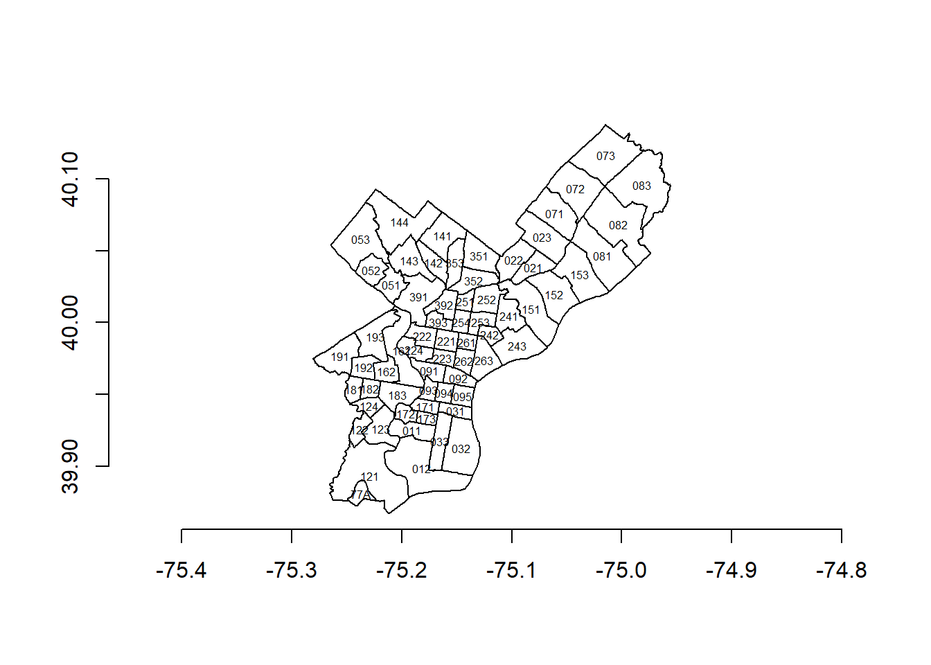
We can extract the actual coordinates of one of the polygons if we wish.
a <- st_coordinates(PPDmap$geometry[1])
head(a)
X Y L1 L2
[1,] -75.00829 40.05272 1 1
[2,] -75.00789 40.05239 1 1
[3,] -75.00616 40.05372 1 1
[4,] -75.00480 40.05476 1 1
[5,] -75.00299 40.05601 1 1
[6,] -75.00118 40.05724 1 1tail(a) X Y L1 L2
[190,] -75.01014 40.05462 1 1
[191,] -75.00921 40.05401 1 1
[192,] -75.00878 40.05366 1 1
[193,] -75.00853 40.05355 1 1
[194,] -75.00851 40.05342 1 1
[195,] -75.00829 40.05272 1 1And we can use those coordinates to add additional features to our plot
plot(st_geometry(PPDmap))
axis(side=1)
axis(side=2)
a <- st_coordinates(st_centroid(st_geometry(PPDmap)))
text(a[,1], a[,2], PPDmap$PSA_NUM, cex=0.5)
a <- st_coordinates(PPDmap$geometry[1])
lines(a[,1], a[,2], col="red", lwd=3)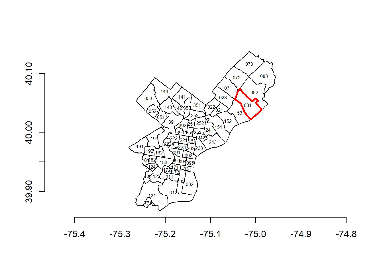
So this highlighted in red PSA 081 in the northern end of Philadelphia.
We can also overlay a leaflet map with the PPDmap object.
leaflet(PPDmap) |>
   addPolygons(weight=1, label=~PSA_NUM) |>
   addTiles()
Geographic datasets that describe locations on the surface of the earth have a “coordinate reference system” (CRS). Let’s extract the CRS for PPDmap.
st_crs(PPDmap)Coordinate Reference System:
User input: 4326
wkt:
GEOGCS["WGS 84",
DATUM["WGS_1984",
SPHEROID["WGS 84",6378137,298.257223563,
AUTHORITY["EPSG","7030"]],
AUTHORITY["EPSG","6326"]],
PRIMEM["Greenwich",0,
AUTHORITY["EPSG","8901"]],
UNIT["degree",0.0174532925199433,
AUTHORITY["EPSG","9122"]],
AXIS["Latitude",NORTH],
AXIS["Longitude",EAST],
AUTHORITY["EPSG","4326"]]The coordinate system used to describe the PPD boundaries is the World Geodetic System 1984 (WGS84) maintained by the United States National Geospatial-Intelligence Agency, one of several standards to aid in navigation and geography. The European Petroleum Survey Group (EPSG) maintains a catalog of different coordinate systems (should be no surprise that oil exploration has driven the development of high quality geolocation standards). They have assigned the standard longitude/latitude coordinate system to be [EPSG4326]((http://spatialreference.org/ref/epsg/4326/). You can find the full collection of coordinate systems at spatialreference.org. You can see in the output above a reference to EPSG 4326.
Many of us are comfortable with the longitude/latitude angular coordinate systems. However, the distance covered by a degree of longitude shrinks as you move towards the poles and only equals the distance covered by a degree of latitude at the equator. In addition, the earth is not very spherical so the coordinate system used for computing distances on the earth surface might need to depend on where you are on the earth surface.
Almost all web mapping tools (Google Maps, ESRI, OpenStreetMaps) use the pseudo-Mercator projection (EPSG3857). Let’s convert our PPD map to that coordinate system.
PPDmap <- st_transform(PPDmap, crs=3857)
st_crs(PPDmap)
Coordinate Reference System:
User input: EPSG:3857
wkt:
PROJCRS["WGS 84 / Pseudo-Mercator",
BASEGEOGCRS["WGS 84",
ENSEMBLE["World Geodetic System 1984 ensemble",
MEMBER["World Geodetic System 1984 (Transit)"],
MEMBER["World Geodetic System 1984 (G730)"],
MEMBER["World Geodetic System 1984 (G873)"],
MEMBER["World Geodetic System 1984 (G1150)"],
MEMBER["World Geodetic System 1984 (G1674)"],
MEMBER["World Geodetic System 1984 (G1762)"],
MEMBER["World Geodetic System 1984 (G2139)"],
ELLIPSOID["WGS 84",6378137,298.257223563,
LENGTHUNIT["metre",1]],
ENSEMBLEACCURACY[2.0]],
PRIMEM["Greenwich",0,
ANGLEUNIT["degree",0.0174532925199433]],
ID["EPSG",4326]],
CONVERSION["Popular Visualisation Pseudo-Mercator",
METHOD["Popular Visualisation Pseudo Mercator",
ID["EPSG",1024]],
PARAMETER["Latitude of natural origin",0,
ANGLEUNIT["degree",0.0174532925199433],
ID["EPSG",8801]],
PARAMETER["Longitude of natural origin",0,
ANGLEUNIT["degree",0.0174532925199433],
ID["EPSG",8802]],
PARAMETER["False easting",0,
LENGTHUNIT["metre",1],
ID["EPSG",8806]],
PARAMETER["False northing",0,
LENGTHUNIT["metre",1],
ID["EPSG",8807]]],
CS[Cartesian,2],
AXIS["easting (X)",east,
ORDER[1],
LENGTHUNIT["metre",1]],
AXIS["northing (Y)",north,
ORDER[2],
LENGTHUNIT["metre",1]],
USAGE[
SCOPE["Web mapping and visualisation."],
AREA["World between 85.06°S and 85.06°N."],
BBOX[-85.06,-180,85.06,180]],
ID["EPSG",3857]]The CRS now indicates that this is a Mercator projection with distance measured in meters (LENGTHUNIT["metre",1]). Now if we ask for the centroids of the PSAs, we get more accurate centroids and no warnings from R.
st_centroid(st_geometry(PPDmap))Geometry set for 65 features
Geometry type: POINT
Dimension: XY
Bounding box: xmin: -8377443 ymin: 4848633 xmax: -8346907 ymax: 4882882
Projected CRS: WGS 84 / Pseudo-Mercator
First 5 geometries:There is a special coordinate system for every part of the world. A useful coordinate system for the Philadelphia area is EPSG2272. Let’s convert our PPD map to that coordinate system.
PPDmap <- st_transform(PPDmap, crs=2272)
st_crs(PPDmap)
Coordinate Reference System:
User input: EPSG:2272
wkt:
PROJCRS["NAD83 / Pennsylvania South (ftUS)",
BASEGEOGCRS["NAD83",
DATUM["North American Datum 1983",
ELLIPSOID["GRS 1980",6378137,298.257222101,
LENGTHUNIT["metre",1]]],
PRIMEM["Greenwich",0,
ANGLEUNIT["degree",0.0174532925199433]],
ID["EPSG",4269]],
CONVERSION["SPCS83 Pennsylvania South zone (US survey foot)",
METHOD["Lambert Conic Conformal (2SP)",
ID["EPSG",9802]],
PARAMETER["Latitude of false origin",39.3333333333333,
ANGLEUNIT["degree",0.0174532925199433],
ID["EPSG",8821]],
PARAMETER["Longitude of false origin",-77.75,
ANGLEUNIT["degree",0.0174532925199433],
ID["EPSG",8822]],
PARAMETER["Latitude of 1st standard parallel",40.9666666666667,
ANGLEUNIT["degree",0.0174532925199433],
ID["EPSG",8823]],
PARAMETER["Latitude of 2nd standard parallel",39.9333333333333,
ANGLEUNIT["degree",0.0174532925199433],
ID["EPSG",8824]],
PARAMETER["Easting at false origin",1968500,
LENGTHUNIT["US survey foot",0.304800609601219],
ID["EPSG",8826]],
PARAMETER["Northing at false origin",0,
LENGTHUNIT["US survey foot",0.304800609601219],
ID["EPSG",8827]]],
CS[Cartesian,2],
AXIS["easting (X)",east,
ORDER[1],
LENGTHUNIT["US survey foot",0.304800609601219]],
AXIS["northing (Y)",north,
ORDER[2],
LENGTHUNIT["US survey foot",0.304800609601219]],
USAGE[
SCOPE["Engineering survey, topographic mapping."],
AREA["United States (USA) - Pennsylvania - counties of Adams; Allegheny; Armstrong; Beaver; Bedford; Berks; Blair; Bucks; Butler; Cambria; Chester; Cumberland; Dauphin; Delaware; Fayette; Franklin; Fulton; Greene; Huntingdon; Indiana; Juniata; Lancaster; Lawrence; Lebanon; Lehigh; Mifflin; Montgomery; Northampton; Perry; Philadelphia; Schuylkill; Snyder; Somerset; Washington; Westmoreland; York."],
BBOX[39.71,-80.53,41.18,-74.72]],
ID["EPSG",2272]]This coordinate system is the Lambert Conic Conformal (LCC). This particular projection of the PPDmap is tuned to provide good precision for the southern part of Pennsylvania (note the parallel coordinates are at the latitude of southern Pennsylvania and the meridian is a little west of Philadelphia) and distances are measured in feet (note the LENGTHUNIT["US survey foot",0.304800609601219] tag in the CRS description).
Let’s transform back to longitude/latitude. It really is best to work using a different coordinate system, but I’m going to stick with longitude/latitude so that the values make a little more sense to us.
PPDmap <- st_transform(PPDmap, crs=4326)Now both PPD data and polygons are on the same scale
plot(st_geometry(PPDmap), axes=TRUE)
points(lat~lon, data=ois, col=rgb(1,0,0,0.5), pch=16)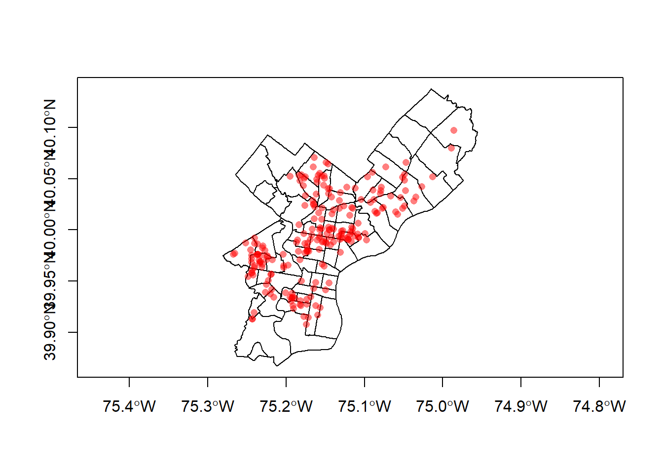
To make the dots a little transparent, I’ve used the rgb() function with which you can mix red, green, and blue colors and set the transparency. The 1 tells rgb() to use maximum red. The two 0s tell rgb() to use no green or blue. The 0.5 tells rgb() to make the dots halfway transparent.
6 Spatial joins
Spatial joins is the process of linking two data sources by their geography. For the case of the OIS data, we want to know how many OISs occurred in each PSA. To do this we need to drop each OIS point location into the PSA polygons and have R tell us in which polygon did each OIS land.
First we need to convert our ois data frame to an sf object, communicating to R that the lon and lat columns are special. At this stage we also have to communicate in what coordinate system are the lon and lat values. st_as_sf() converts an R object into an sf object.
ois <- st_as_sf(ois,
                coords=c("lon","lat"),
                crs=4326)
ois |> select(-text)
Simple feature collection with 219 features and 8 fields
Geometry type: POINT
Dimension: XY
Bounding box: xmin: -75.26743 ymin: 39.90737 xmax: -74.98606 ymax: 40.09692
Geodetic CRS: WGS 84
First 10 features:
id date location year
1 24-22 2024-06-24 6150 West Columbia Avenue, Philadelphia, PA 2024
2 24-21 2024-06-22 3550 F Street, Philadelphia, PA 2024
3 24-20 2024-06-15 2750 North 6th Street, Philadelphia, PA 2024
4 24-18 2024-06-05 1550 North 57th Street, Philadelphia, PA 2024
5 24-17 2024-05-30 2150 East Westmoreland Street, Philadelphia, PA 2024
6 24-15 2024-05-23 1600 South Dover Street, Philadelphia, PA 2024
7 24-14 2024-05-15 3050 North 16th Street , Philadelphia, PA 2024
8 24-13 2024-05-14 1550 58th Street, Philadelphia, PA 2024
9 24-12 2024-05-14 2250 West Oxford Avenue, Philadelphia, PA 2024
10 24-10 2024-05-01 3950 Fairmont Avenue, Philadelphia, PA 2024
url
1 https://ois.sites.phillypolice.com/ps24-22/
2 https://ois.sites.phillypolice.com/ps24-21/
3 https://ois.sites.phillypolice.com/ps24-20/
4 https://ois.sites.phillypolice.com/ps24-18/
5 https://ois.sites.phillypolice.com/ps24-17/
6 https://ois.sites.phillypolice.com/ps24-15/
7 https://ois.sites.phillypolice.com/ps24-14/
8 https://ois.sites.phillypolice.com/ps24-13/
9 https://ois.sites.phillypolice.com/ps24-12/
10 https://ois.sites.phillypolice.com/ps24-10/
addrmatch score
1 6150 W Columbia Ave, Philadelphia, Pennsylvania, 19151 100.00
2 3550 F St, Philadelphia, Pennsylvania, 19134 100.00
3 2750 N 6th St, Philadelphia, Pennsylvania, 19133 100.00
4 1550 N 57th St, Philadelphia, Pennsylvania, 19131 100.00
5 2150 E Westmoreland St, Philadelphia, Pennsylvania, 19134 100.00
6 1600 S Dover St, Philadelphia, Pennsylvania, 19145 100.00
7 3050 N 16th St, Philadelphia, Pennsylvania, 19132 100.00
8 1550 N 58th St, Philadelphia, Pennsylvania, 19131 99.50
9 2250 W Oxford St, Philadelphia, Pennsylvania, 19121 97.85
10 3950 Fairmount Ave, Philadelphia, Pennsylvania, 19104 97.64
addrtype geometry
1 PointAddress POINT (-75.24509 39.98057)
2 StreetAddress POINT (-75.11626 40.00266)
3 StreetAddress POINT (-75.14207 39.99318)
4 PointAddress POINT (-75.23549 39.97601)
5 PointAddress POINT (-75.10709 39.99267)
6 StreetAddress POINT (-75.19237 39.9335)
7 PointAddress POINT (-75.15671 40.0002)
8 PointAddress POINT (-75.23695 39.97583)
9 StreetAddress POINT (-75.17245 39.97906)
10 StreetAddress POINT (-75.20275 39.9651)You can see that ois now has one of those special geometry columns. We can plot the OISs on the map.
plot(st_geometry(PPDmap), axes=TRUE)
plot(st_geometry(ois), add=TRUE, col=rgb(1,0,0,0.5), pch=16)
st_join() will match each row in ois to each polygon in PSA. I just want to add the PSA_NUM column out of the PPDmap.
PSAlookup <- ois |>
  st_join(PPDmap |> select(PSA_NUM))
PSAlookup |>
   select(id, date, location, PSA_NUM, geometry) |>
   head()
Simple feature collection with 6 features and 4 fields
Geometry type: POINT
Dimension: XY
Bounding box: xmin: -75.24509 ymin: 39.9335 xmax: -75.10709 ymax: 40.00266
Geodetic CRS: WGS 84
id date location PSA_NUM
1 24-22 2024-06-24 6150 West Columbia Avenue, Philadelphia, PA 191
2 24-21 2024-06-22 3550 F Street, Philadelphia, PA 253
3 24-20 2024-06-15 2750 North 6th Street, Philadelphia, PA 254
4 24-18 2024-06-05 1550 North 57th Street, Philadelphia, PA 192
5 24-17 2024-05-30 2150 East Westmoreland Street, Philadelphia, PA 243
6 24-15 2024-05-23 1600 South Dover Street, Philadelphia, PA 172
geometry
1 POINT (-75.24509 39.98057)
2 POINT (-75.11626 40.00266)
3 POINT (-75.14207 39.99318)
4 POINT (-75.23549 39.97601)
5 POINT (-75.10709 39.99267)
6 POINT (-75.19237 39.9335)Now our PSAlookup contains everything from ois but also adds a new column PSA_NUM.
Let’s examine the PSAs with the most OISs and highlight them on the map.
a <- rev(sort(table(PSAlookup$PSA)))
a
192 221 242 253 151 141 254 172 142 391 353 222 153 011 252 224 193 191 181 152
 18  10   9   8   8   8   7   7   7   6   6   6   6   6   5   5   5   5   5   5
393 392 261 162 021 352 243 241 173 124 033 022 351 251 182 161 143 123 121 092
  4   4   4   4   4   3   3   3   3   3   3   3   2   2   2   2   2   2   2   2
081 031 023 012 263 223 183 122 095 094 093 091 083 082 071 032
2 2 2 2 1 1 1 1 1 1 1 1 1 1 1 1 plot(st_geometry(PPDmap), axes=TRUE)
PSAlookup |>
filter(PSA_NUM=="192") |>
st_geometry() |>
plot(add=TRUE, col=rgb(0,1,0,0.5), pch=16)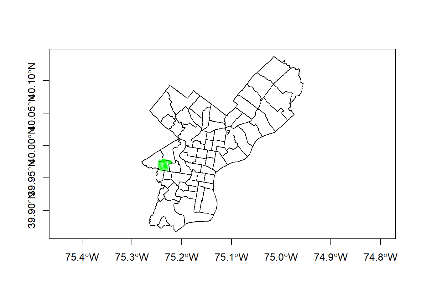
Let’s identify which OISs occurred in the same PSA as the University of Pennsylvania. We’ve already geocoded Penn and have its coordinates. Let’s join it with PPDmap to find out which PSA it is in.
gcPenn address location.x location.y
1 3718 Locust Walk, Philadelphia, Pennsylvania, 19104 -75.19758 39.95227
score attributes.Match_addr
1 100 3718 Locust Walk, Philadelphia, Pennsylvania, 19104
attributes.Addr_type extent.xmin extent.ymin extent.xmax extent.ymax
1 StreetAddress -75.19858 39.95127 -75.19658 39.95327
lon lat
1 -75.19758 39.95227st_as_sf(gcPenn,
coords=c("lon","lat"),
crs=4326) |>
st_join(PPDmap) |>
select(PSA_NUM)Simple feature collection with 1 feature and 1 field
Geometry type: POINT
Dimension: XY
Bounding box: xmin: -75.19758 ymin: 39.95227 xmax: -75.19758 ymax: 39.95227
Geodetic CRS: WGS 84
PSA_NUM geometry
1 183 POINT (-75.19758 39.95227)Now we see that Penn is in PSA 183 and we can highlight those points on the map.
plot(st_geometry(PPDmap), axes=TRUE)
PSAlookup |>
  filter(PSA_NUM=="183") |>
  st_geometry() |>
  plot(add=TRUE, col="blue", pch=16)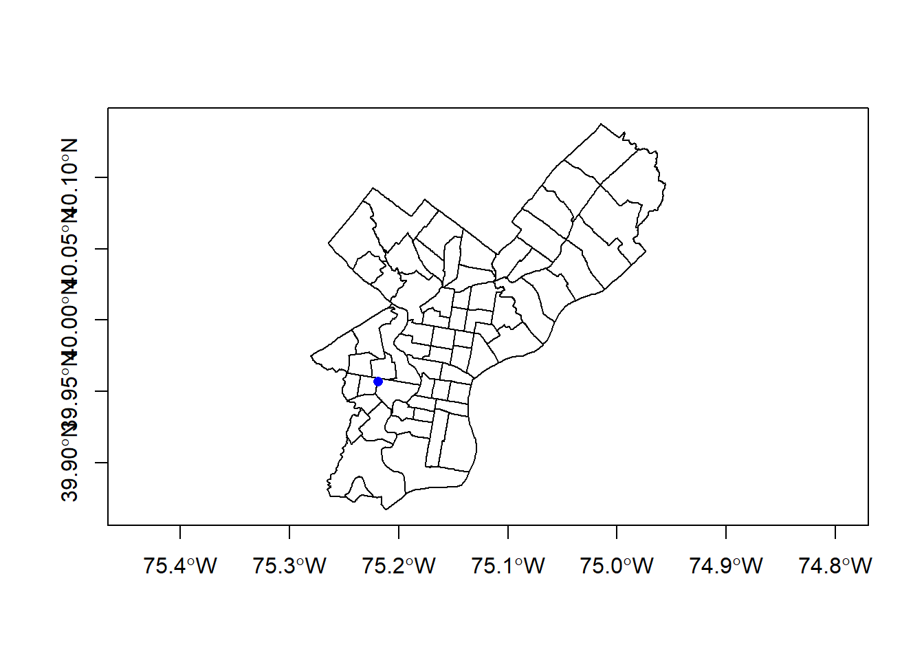
You can learn more about the incident near Penn.
# read more about incidents in PSA 183
PSAlookup |>
  filter(PSA_NUM=="183") |>
  select(text) |>
   st_drop_geometry()
text
1 PS#16-30\n9/16/16\nOn Friday, September 16, 2016, at approximately 11:18 P.M., a uniformed sergeant in a marked police vehicle was seated in her parked vehicle in the 5100 block of Sansom Street, when a male approached and without warning, began to discharge a firearm, striking the sergeant, as she remained seated in her vehicle. The offender then began walking east on Sansom Street, stopping at a lounge/bar in the 5100 block of Sansom Street, where he discharged his firearm into the lounge/bar, striking a female employee and a male security guard. The offender continued walking east on Sansom Street to the 4900 block, where he discharged his firearm into an occupied parked vehicle, striking one female and one male occupant.\nResponding uniformed officers, in marked police vehicles, along with an officer from the University of Pennsylvania police force, located the offender in an alleyway in the rear of the 4800 blocks of Sansom and Walnut Streets. While in the 4800 block of Sansom Street the offender discharged his firearm, striking the University of Pennsylvania Officer as well as a marked police vehicle. Four Officers (one of whom was the University of Pennsylvania Officer) discharged their firearms, striking the offender. The offender fell to the ground and dropped his firearm. Fire Rescue responded and pronounced the offender deceased. \nThe offender’s firearm, a 9MM, semi-automatic pistol, with an obliterated serial number, loaded with 14 live rounds, was recovered at the scene. There were three empty magazines from the offender’s firearm recovered throughout the scene. \nThe sergeant, the University of Pennsylvania Officer, along with the four civilians who were all struck by gunfire, were transported to Penn-Presbyterian Hospital for treatment.\nThe female from the parked vehicle was later pronounced deceased at Penn-Presbyterian Hospital.\n*** Information posted in the original summary reflects a preliminary understanding of what occurred at the time of the incident. This information is posted shortly after the incident and may be updated as the investigation leads to new information. The DA’s Office is provided all the information from the PPD’s investigation prior to their charging decision.Lastly, we will tabulate the number of OISs in each PSA and color the map by the number of OISs.
# how many shootings in each PSA?
a <- PSAlookup |>
  count(PSA_NUM) |>
  st_drop_geometry()

# merge the shooting count into the PPDmap data
PPDmap <- PPDmap |>
  left_join(a, by=join_by(PSA_NUM)) |>
  rename(nShoot=n) |>
  mutate(nShoot=replace_na(nShoot, 0))

head(PPDmap)
Simple feature collection with 6 features and 13 fields
Geometry type: POLYGON
Dimension: XY
Bounding box: xmin: -75.19317 ymin: 39.94528 xmax: -74.95575 ymax: 40.12047
Geodetic CRS: WGS 84
OBJECTID DISTRICT__ DESCRIPT AREA PERIMETER PSACOV_ PSACOV_ID ID
1 1 08 136213942 56995.90 <NA> <NA> 16
2 2 08 168027734 66474.25 <NA> <NA> 17
3 3 08 169959462 66663.50 <NA> <NA> 18
4 4 09 32508297 15689.07 <NA> <NA> 19
5 5 09 29214098 15689.07 <NA> <NA> 19
6 6 09 19008247 15689.07 <NA> <NA> 19
Shape__Area PSA_NUM OLD_SECTOR Shape__Length nShoot
1 21620450 081 A,B,E,F,L,M 22713.821 2
2 26686944 082 C,G,H,I,N 26496.596 1
3 27015453 083 D,J,K,O,P 26581.340 1
4 5147735 091 A,B,C,D,E,F 11292.247 1
5 4625366 092 A,B,C,D,E,F 10643.107 2
6 3008753 093 A,B,C,D,E,F 8243.953 1
geometry
1 POLYGON ((-75.00829 40.0527...
2 POLYGON ((-74.99876 40.0813...
3 POLYGON ((-74.97567 40.1202...
4 POLYGON ((-75.1597 39.97021...
5 POLYGON ((-75.13524 39.9507...
6 POLYGON ((-75.16716 39.9587...We can see that PPDmap now has a new nShoot column. A histogram will show what kinds of counts we observe in the PSAs.
hist(a$n, xlab="Number of OISs", ylab="Number of PSAs", main="")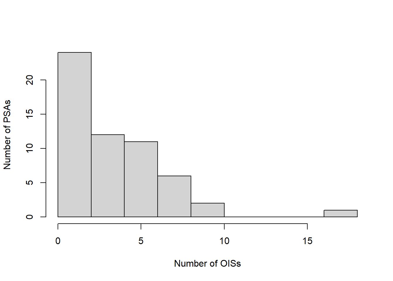
Let’s discretize the OIS counts into a few categories.
PPDmap <- PPDmap |>
  mutate(catShoot =
           cut(nShoot,
               breaks=c(0,1,2,3,4,8,Inf),
               right=FALSE))
cut() converts all of the individual counts into categories, like [1,5) or [25,30). For each of these categories we will associate a color for the map. heat.colors() will generate a sequence of colors in the yellow, orange, red range.
a <- data.frame(catShoot=levels(PPDmap$catShoot),
                col=rev(heat.colors(6,1)))
a
# some other color options
#    col = rev(rainbow(6,1))
#    or generate a range of red colors
#    col = rgb(seq(0,1,length=6),0,0,1)
catShoot col
1 [0,1) #FFFF80FF
2 [1,2) #FFFF00FF
3 [2,3) #FFBF00FF
4 [3,4) #FF8000FF
5 [4,8) #FF4000FF
6 [8,Inf) #FF0000FFThese are eight digit codes describing the color. The first two digits correspond to red, digits three and four correspond to green, digits five and six correspond to blue, and the last two digits correspond to transparency. These are hexadecimal numbers (base 16). Hexadecimal numbers use the digits 0-9, like normal decimal system numbers, and then denote 10 as A, 11 as B, on up to 15 as F. So FF as a decimal is \(15 \times 16 + 15 = 255\), which is the maximum value for a two digit hexadecimal. The hexadecimal 80 as a decimal is \(8 \times 16 + 0 = 128\), which is in the middle of the range 0 to 255. So the first color code, FFFF80FF, means maximum red, maximum green, half blue, and not transparent at all. This mixture is known more commonly as “yellow”.
Now we join PPDmap with our color lookup table in a and plot it.
# match the color to category
PPDmap <- PPDmap |>
  left_join(a, by=join_by(catShoot))

PPDmap |>
  st_geometry() |>
  plot(col=PPDmap$col, border="black")
# add the number of shootings
b <- st_coordinates(st_centroid(PPDmap))
Warning: st_centroid assumes attributes are constant over geometriestext(b[,1], b[,2], PPDmap$nShoot, cex=0.7)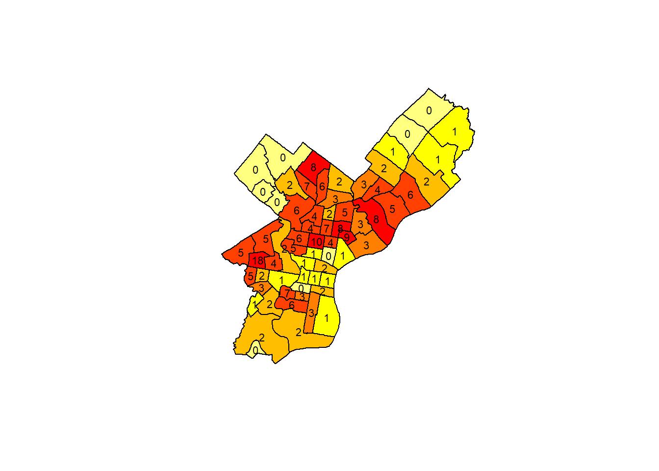
Those PSAs with the least shootings are a very pale yellow. As we examine PSAs with a greater number of OISs, their colors get redder and redder.
And a leaflet version to end on.
PPDmap <- PPDmap |>
  mutate(label = paste("PSA:",PSA_NUM, "Count:",nShoot))

leaflet(PPDmap) |>
   addPolygons(weight=1, col=~col, label=~label) |>
   addTiles()
7 Summary
We started with just a web page linking to a collection of pdf files. We used regular expressions to extract everything we could from the web page tables. We had R “read” the pdf files to extract the dates that were not readily available. We geocoded the stops so that we could put them on a map. Finally, we could tabulate by PSA the number of OISs and map those as well.
If you’ve worked through all of this, then I would recommend that you save your objects, using save(ois, PSAlookup, gcOIS, file="PPDOIS.RData"). That way you will not have to scrape everything off the web again or redo any geocoding.
8 Exercises
Revisit the geocoding section discussing geocoding errors. Examine the OISs that have not been geocoded to specific locations. Fix their addresses and redo the geocoding of these OISs to improve the accuracy of the data.
Identify officer-involved shootings that resulted in the offender being transported to the Hospital at the University of Pennsylvania. Create a map marking the location of HUP, the location of officer-involved shootings resulting in the offender being transported to HUP, and the locations of all other shootings.
For each shooting determine which hospital treated the offender. Use
st_distance()to determine what percentage of those shot in an OIS went to the closest hospital.