DupSeq_QC_Lane11

Last updated: 2022-08-27

Checks: 6 1

Knit directory: duplex_sequencing_screen/

This reproducible R Markdown analysis was created with workflowr (version 1.6.2). The Checks tab describes the reproducibility checks that were applied when the results were created. The Past versions tab lists the development history.

R Markdown file: uncommitted changes

The R Markdown file has unstaged changes. To know which version of the R Markdown file created these results, you’ll want to first commit it to the Git repo. If you’re still working on the analysis, you can ignore this warning. When you’re finished, you can run wflow_publish to commit the R Markdown file and build the HTML.

Environment: empty

Great job! The global environment was empty. Objects defined in the global environment can affect the analysis in your R Markdown file in unknown ways. For reproduciblity it’s best to always run the code in an empty environment.

Seed: set.seed(20200402)

The command set.seed(20200402) was run prior to running the code in the R Markdown file. Setting a seed ensures that any results that rely on randomness, e.g. subsampling or permutations, are reproducible.

Session information: recorded

Great job! Recording the operating system, R version, and package versions is critical for reproducibility.

Cache: none

Nice! There were no cached chunks for this analysis, so you can be confident that you successfully produced the results during this run.

File paths: relative

Great job! Using relative paths to the files within your workflowr project makes it easier to run your code on other machines.

Repository version: d5adfc5

Great! You are using Git for version control. Tracking code development and connecting the code version to the results is critical for reproducibility.

The results in this page were generated with repository version d5adfc5. See the Past versions tab to see a history of the changes made to the R Markdown and HTML files.

Note that you need to be careful to ensure that all relevant files for the analysis have been committed to Git prior to generating the results (you can use wflow_publish or wflow_git_commit). workflowr only checks the R Markdown file, but you know if there are other scripts or data files that it depends on. Below is the status of the Git repository when the results were generated:


Ignored files:
    Ignored:    .Rhistory
    Ignored:    .Rproj.user/
    Ignored:    data/Consensus_Data/.Rhistory
    Ignored:    data/Consensus_Data/Novogene_lane2/abl_ref/kraken2-master/newdir/
    Ignored:    data/Consensus_Data/Novogene_lane4/.ipynb_checkpoints/
    Ignored:    data/Consensus_Data/Novogene_lane4/GalaxyData/initialanalysis/
    Ignored:    data/Consensus_Data/Novogene_lane4/output/
    Ignored:    data/Consensus_Data/Novogene_lane6/
    Ignored:    data/Consensus_Data/Novogene_lane7/
    Ignored:    data/Consensus_Data/Ranomics_Pooled/RP4/
    Ignored:    data/Consensus_Data/Ranomics_Pooled/RP5/

Untracked files:
    Untracked:  analysis/figure/
    Untracked:  data/Consensus_Data/Novogene_lane11/sample2/variants_ann_sample2.csv
    Untracked:  data/Consensus_Data/Novogene_lane11/sample2/variants_unique_ann_sample2.csv
    Untracked:  data/Consensus_Data/Novogene_lane11/sample6/twinstrand pipeline outputs/.DS_Store
    Untracked:  data/Consensus_Data/Novogene_lane11/sample6/variant_caller_outputs/
    Untracked:  data/Consensus_Data/Novogene_lane12/sample1/.DS_Store
    Untracked:  data/Consensus_Data/Novogene_lane12/sample1/low_sscscounts/
    Untracked:  data/Consensus_Data/Novogene_lane12/sample1/sscs_aligned_filtered.tsv
    Untracked:  data/Consensus_Data/Novogene_lane12/sample1/variant_caller_outputs/
    Untracked:  data/Consensus_Data/Novogene_lane12/sample3/
    Untracked:  data/Consensus_Data/Novogene_lane12/sample5/
    Untracked:  data/Consensus_Data/Novogene_lane12/sample7/
    Untracked:  data/Consensus_Data/Novogene_lane12/sample9/

Unstaged changes:
    Modified:   .DS_Store
    Modified:   analysis/DupSeq_QC_Lane11.Rmd
    Modified:   analysis/variant_caller_2022.Rmd
    Modified:   code/.DS_Store
    Modified:   code/variantcaller/vep_fromdf.R
    Modified:   code/variantcaller/vep_fromdf_parralel.R
    Modified:   data/Consensus_Data/.DS_Store
    Modified:   data/Consensus_Data/Novogene_lane11/.DS_Store
    Deleted:    data/Consensus_Data/Novogene_lane11/sample2/sscs_reads_ann.csv
    Deleted:    data/Consensus_Data/Novogene_lane11/sample2/sscs_sum_ann.csv
    Modified:   data/Consensus_Data/Novogene_lane11/sample6/.DS_Store
    Deleted:    data/Consensus_Data/Novogene_lane11/sample6/twinstrand pipeline outputs/variants_ann_sample5&6.csv
    Deleted:    data/Consensus_Data/Novogene_lane11/sample6/twinstrand pipeline outputs/variants_ann_sample6.csv.gz
    Deleted:    data/Consensus_Data/Novogene_lane11/sample6/twinstrand pipeline outputs/variants_unique_ann_sample5&6.csv
    Deleted:    data/Consensus_Data/Novogene_lane11/sample6/twinstrand pipeline outputs/variants_unique_ann_sample6.csv
    Modified:   data/Consensus_Data/Novogene_lane12/.DS_Store
    Deleted:    data/Consensus_Data/Novogene_lane12/sample1/sscs_aligned_filtered.tsv.gz
    Modified:   data/Consensus_Data/archive/.DS_Store
    Modified:   data/Refs/.DS_Store
    Modified:   data/Refs/ABL/NM_005157.6_CDS.txt

Note that any generated files, e.g. HTML, png, CSS, etc., are not included in this status report because it is ok for generated content to have uncommitted changes.

These are the previous versions of the repository in which changes were made to the R Markdown (analysis/DupSeq_QC_Lane11.Rmd) and HTML (docs/DupSeq_QC_Lane11.html) files. If you’ve configured a remote Git repository (see ?wflow_git_remote), click on the hyperlinks in the table below to view the files as they were in that past version.

File	Version	Author	Date	Message
Rmd	fecc2e4	haiderinam	2022-08-23	August 2022 Updates
Rmd	7ed0af8	haiderinam	2022-08-22	August 2022 Updates

In the following chunks, I’m going to be doing some QC with the duplex sequencing data from novogene lane 11 This sequencing run had both EGFR and ABL data. The libraries are twist libraries.

I’m going to be looking closely at the following:
* Count distributions of EGFR vs ABL * How much coverage do we get with a single sample of EGFR vs with two samples? Answer: 100k for 1 sample, 200k for two SSCS samples * What is the % on-target? * What is the % N? * What is the % of split reads? * What is the % mouse?

How much coverage do we get for DCS vs for SSCS? Answer: For a dupseq coverage of 40k, our SSCS coverage was 100k This is a very low % of SSCS reads that are orphaned. For schmitt’s adapter types, about 80-90% of the SSCS reads are orphaned.
What is the error rate for SSCS vs for DCS? Answer:
What is the % of mouse reads that we’re seeing for the samples? Answer: Mouse read %age is very low for EGFR (1% of the barcodes align to the mouse genome). For ABL, between 1 and 30% of the consensus reads align to the mouse genome
How many unique mutants do we see for EGFR? What percent coverage is that? Answer: Combining two EGFR samples at the baseline and using SSCS counts, we achieve a coverage of 200k. At this coverage, we’re seeing 2340 out of 2700 mutants that twist’s QC data saw. That’s 90% of the mutants at baseline.
What is the count distribution of the mutants in the data? aka how many times do we see each mutant? Answer:
How many unique mutants do you see per 10k barcodes sequenced? How does downsampling influence the sequencing data output? Answer:
How well do the mutant allele frequencies agree with twist’s MAFs?
How many reads/consensus barcodes are taken up by each of the residues?
What percent of the barcodes are taken up by the top 10 mutants? What about the top 50 mutants?
Modify the function so that you’re not relying on ensembl’s VEP.

####Novogene Lane 12####

####Novogene Lane 11#### Sample 6

# getwd()
# sample5_all=read.csv("data/Consensus_Data/Novogene_lane11/sample5/variants_ann_sample5.csv")
sample5_sum=read.csv("data/Consensus_Data/Novogene_lane11/sample5/variant_caller_outputs/variants_unique_ann_sample5.csv")
# sample5_all=read.csv("data/Consensus_Data/Novogene_lane11/sample5/variants_ann_sample5.csv")
# a=sample5_all%>%filter(protein_start%in%903,ref%in%"T",alt%in%"C")

# sample6_all=read.csv("data/Consensus_Data/Novogene_lane11/sample6/variants_ann_sample5&6.csv")
sample6_sum=read.csv("data/Consensus_Data/Novogene_lane11/sample6/variant_caller_outputs/variants_unique_ann_sample6.csv")
sample5_simple=sample5_sum%>%dplyr::select(alt_start_pos,protein_start,ref,alt,consequence_terms,amino_acids,ct,depth)
sample5_simple$sample="sample5"
sample6_simple=sample6_sum%>%dplyr::select(alt_start_pos,protein_start,ref,alt,consequence_terms,amino_acids,ct,depth)
sample6_simple$sample="sample6"
sample56=rbind(sample5_simple,sample6_simple)
# a=sample56%>%filter(protein_start>=715,protein_start<=900,consequence_terms%in%"missense_variant")
plotly=ggplot(sample56%>%filter(protein_start>=715,protein_start<=900,consequence_terms%in%"missense_variant"),aes(x=protein_start,y=depth,fill=sample))+geom_col(position=position_dodge())+facet_wrap(~sample)+cleanup
ggplotly(plotly)

Warning: `group_by_()` was deprecated in dplyr 0.7.0.
Please use `group_by()` instead.
See vignette('programming') for more help

sample56_merged=merge(sample5_simple,sample6_simple,by=c("alt_start_pos","protein_start","ref","alt","consequence_terms","amino_acids"),all.x = T)

# a=sample56_merged%>%filter(depth.x>=1000,protein_start>=715,protein_start<=870,consequence_terms%in%"missense_variant")
sample56_merged[sample56_merged$ct.y%in%NA,10]=1000
sample56_merged[sample56_merged$depth.y%in%NA,11]=1000
# sample56_merged=sample56_merged%>%
#   rowwise()%>%
#   mutate(ct.y=case_when(ct.y%in%NA~0,
#                         T~ct.y))
ggplot(sample56_merged%>%filter(depth.x>=1000,protein_start>=715,protein_start<=870,consequence_terms%in%"missense_variant"),aes(x=ct.x/depth.x,y=ct.y/depth.y))+
  geom_point(color="black",shape=21,aes(fill=log10(ct.x)))+
  scale_x_continuous(trans="log10")+
  scale_y_continuous(trans="log10")+
  cleanup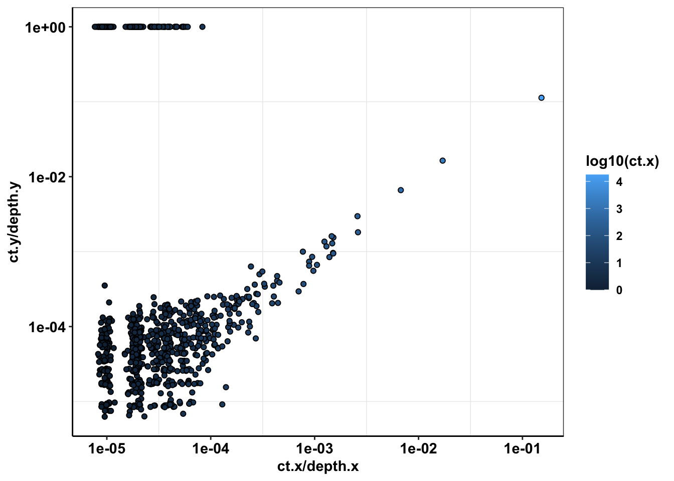

plotly=ggplot(sample5_sum%>%filter(protein_start>=715,protein_start<=870,consequence_terms%in%"missense_variant",ct<=50,type%in%"mnv"),aes(x=ct))+
  geom_histogram(aes(y=..density..),color=1,fill="white",bins=50)+
  geom_density(lwd = 1, colour = 4,fill = 4, alpha = 0.25)
ggplotly(plotly)

plotly=ggplot(sample6_sum%>%filter(protein_start>=715,protein_start<=870,consequence_terms%in%"missense_variant",ct<=50,type%in%"mnv"),aes(x=ct))+
  geom_histogram(aes(y=..density..),color=1,fill="white",bins=50)+
  geom_density(lwd = 1, colour = 4,fill = 4, alpha = 0.25)
  # scale_x_continuous(trans="log10")
ggplotly(plotly)

# a=sample5_sum%>%filter(protein_start>=715,protein_start<=870,consequence_terms%in%"missense_variant",ct==1)
# nrow(a%>%filter(type%in%"mnv"))
# b=sample6_sum%>%filter(protein_start>=715,protein_start<=870,consequence_terms%in%"missense_variant",ct==1)
# nrow(b%>%filter(type%in%"mnv"))
#For sample 5, out of the mutants that are only seen once, 34% are mnvs (a lot of SNP errors). So a lot of the mutants that we are seeing at a coverage of 1 are false. This means that for sample 5, the distribution of mutants is centered >1
#For sample 6, out of the mutants that are only seen once, 62% are mnvs (low SNP errors)

calls_sum=sample5_sum%>%filter(consequence_terms%in%"missense_variant")%>%group_by(protein_start)%>%summarize(unique_mutants=n(),count=sum(ct))
ggplot(calls_sum%>%filter(protein_start>=715,protein_start<=870),aes(x=protein_start,y=unique_mutants))+geom_col()+cleanup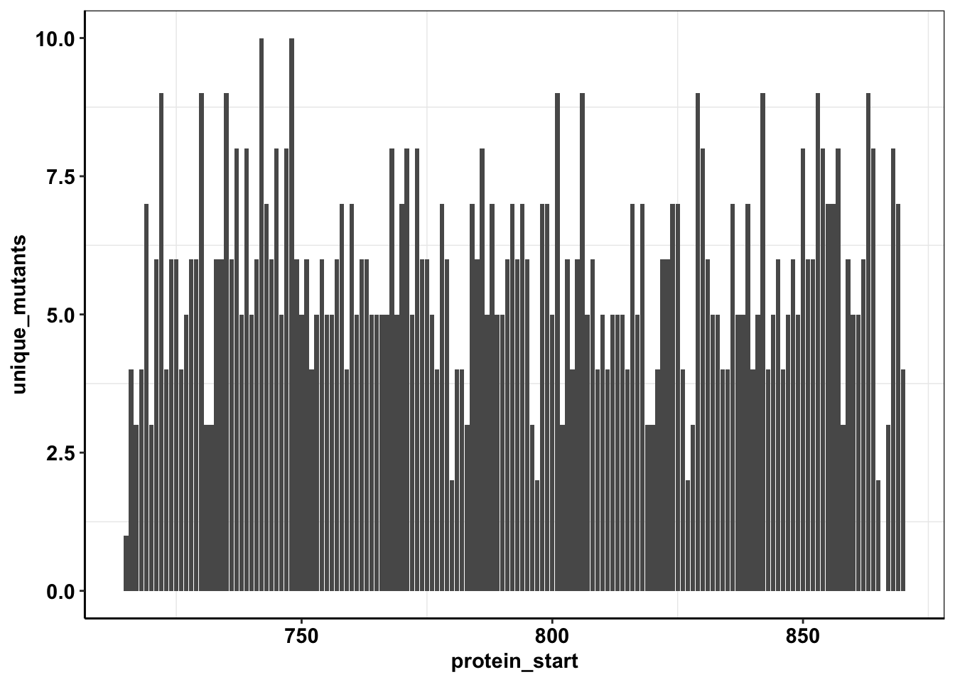

ggplot(calls_sum%>%filter(protein_start>=715,protein_start<=870),aes(x=protein_start,y=count))+geom_col()+cleanup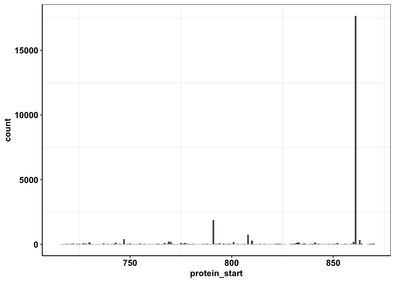

calls_sum=sample6_sum%>%filter(consequence_terms%in%"missense_variant")%>%group_by(protein_start)%>%summarize(unique_mutants=n(),count=sum(ct))
ggplot(calls_sum%>%filter(protein_start>=715,protein_start<=870),aes(x=protein_start,y=unique_mutants))+geom_col()+cleanup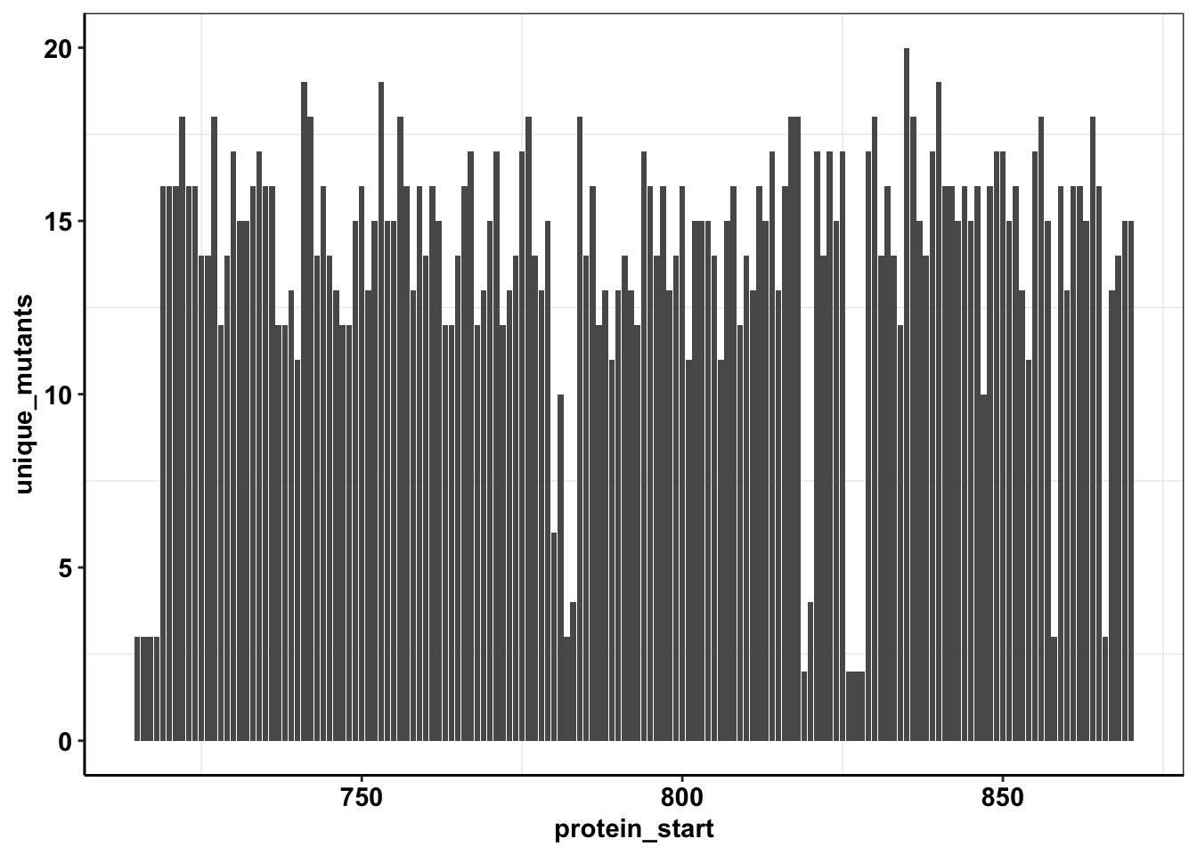

ggplot(calls_sum%>%filter(protein_start>=715,protein_start<=870),aes(x=protein_start,y=count))+geom_col()+cleanup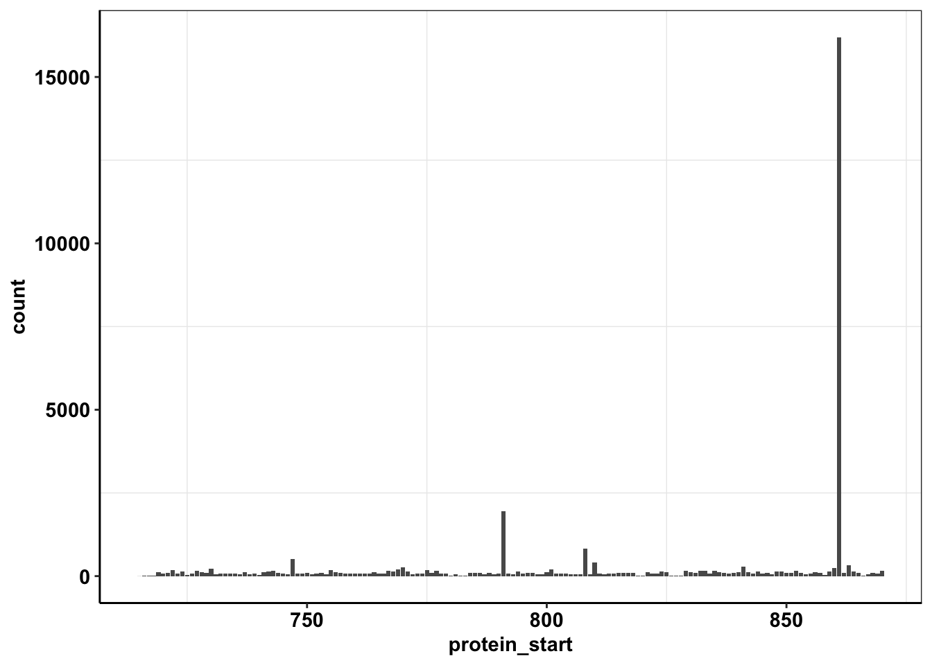

ggplot(calls_sum%>%filter(protein_start>=715,protein_start<=870,!protein_start%in%861),aes(x=protein_start,y=count))+geom_col()+cleanup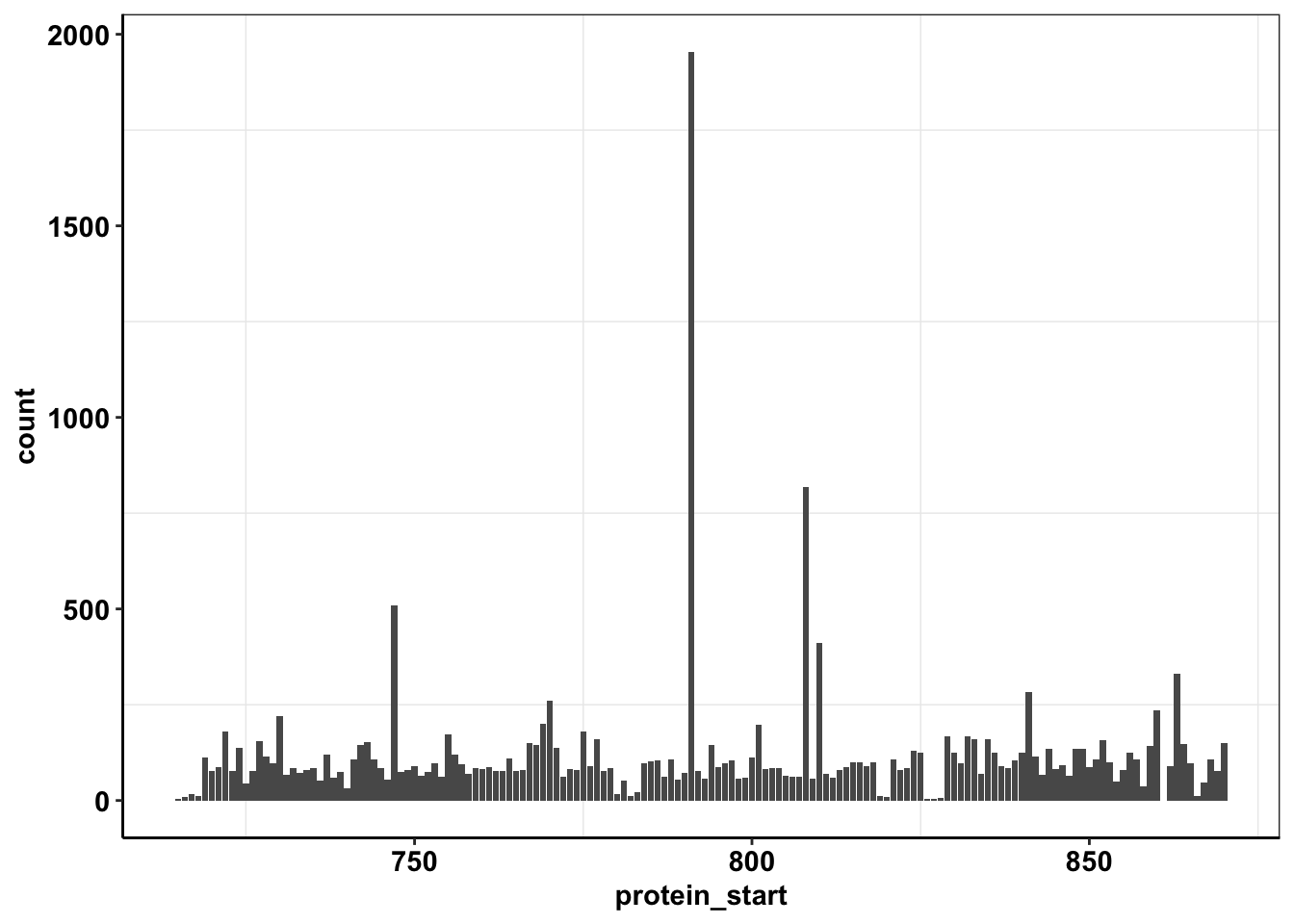

ggplot(calls_sum%>%filter(protein_start>=715,protein_start<=870,!protein_start%in%c(861,791)),aes(x=protein_start,y=count))+geom_col()+cleanup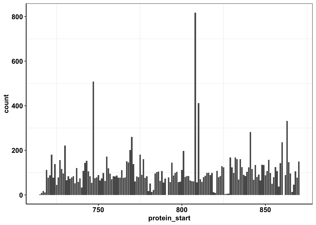

# a=sample5_sum%>%filter(consequence_terms%in%"missense_variant",protein_start>=715,protein_start<=870)
# sum(a$ct)

Sample 6

calls_missense=calls_missense%>%
  filter(protein_start==protein_end,consequence_terms%in%"missense_variant")%>%
  rowwise()%>%
  mutate(ref_aa=strsplit(amino_acids,"/")[[1]][1],
         alt_aa=strsplit(amino_acids,"/")[[1]][2])

ggplot(calls_missense,aes(x=protein_start,y=alt_aa))+
  geom_tile(color="black",aes(fill=(ct/depth)))+
  scale_x_continuous(name="Position along EGFR Kinase",expand=c(0,0),limits=c(717,870))+
  scale_y_discrete(name="Amino Acid Substitution",expand=c(0,0))+
  scale_fill_continuous(name="Allele \nFrequency",trans="log10")+
  cleanup+
  theme(legend.position = "none")
# a=calls_missense%>%filter(protein_start>=715,protein_start<=880)
# ggsave("egfr_heatmap_sample5.pdf",width=6,height=4,units = "in",useDingbats=F)

ggplot(calls_missense_sum,aes(x=protein_start,y=count))+geom_col()+scale_x_continuous(limits=c(710,875))

SAMPLE 2

library("plotly")
sample2_sum=read.csv("data/Consensus_Data/Novogene_lane11/sample2/variants_unique_ann_sample2.csv",header = T,stringsAsFactors = F)[-1]
sample2_sum$consensus="sscs"
sample2_sum=sample2_sum%>%
  # filter(protein_start==protein_end,consequence_terms%in%"missense_variant")%>%
  rowwise()%>%
  mutate(ref_aa=strsplit(amino_acids,"/")[[1]][1],
         alt_aa=strsplit(amino_acids,"/")[[1]][2])

sample2_all=read.csv("data/Consensus_Data/Novogene_lane11/sample2/variants_ann_sample2.csv",header = T,stringsAsFactors = F)[-1]
sample2_all$consensus="sscs"
dcs_sum=read.csv("data/Consensus_Data/Novogene_lane11/sample2/duplex_sum_ann.csv",header = T,stringsAsFactors = F)[-1]
dcs_sum$consensus="dcs"

sample2_all=sample2_all%>%
  # filter(protein_start==protein_end,consequence_terms%in%"missense_variant")%>%
  rowwise()%>%
  mutate(ref_aa=strsplit(amino_acids,"/")[[1]][1],
         alt_aa=strsplit(amino_acids,"/")[[1]][2])
# a=sample2_all%>%filter(protein_start%in%493,amino_acids%in%"F")

sample2_sum

dcs_sum=dcs_sum%>%
  filter(protein_start==protein_end,consequence_terms%in%"missense_variant")%>%
  rowwise()%>%
  mutate(ref_aa=strsplit(amino_acids,"/")[[1]][1],
         alt_aa=strsplit(amino_acids,"/")[[1]][2])

ggplot(sample2_sum,aes(x=protein_start,y=alt_aa))+
  geom_tile(color="black",aes(fill=ct))+
  scale_x_continuous(expand=c(0,0),limits=c(242,333))+
  scale_y_discrete(expand=c(0,0))

all_sum=rbind(sample2_sum,dcs_sum)

plotly=ggplot(all_sum,aes(x=ct,fill=consensus,alpha=0.5))+
  geom_density(position=position_dodge(),bins=100)+
  scale_x_continuous(limits=c(0,100))
  # scale_x_continuous(trans="log10")
ggplotly(plotly)

plotly=ggplot(all_sum,aes(x=ct,fill=consensus,alpha=0.5))+
  geom_density(position=position_dodge(),bins=100)+
  # scale_x_continuous(limits=c(0,100))+
  scale_x_continuous(trans="log10")
ggplotly(plotly)



ggplot(all_sum,aes(x=protein_start,y=alt_aa))+
  geom_tile(color="black",aes(fill=ct))+
  facet_grid(~consensus)+
  scale_x_continuous(expand=c(0,0),limits=c(241,333))+
  scale_y_discrete(expand=c(0,0))+
  scale_fill_gradient(na.value = "black",low="red",high="blue",name="Count")

# a=sscs_sum%>%filter(protein_start>=242,protein_start<=289)
# a=a%>%group_by(protein_start)%>%summarize(count=n())

calls_sum=sample2_sum%>%filter(consequence_terms%in%"missense_variant")%>%group_by(protein_start)%>%summarize(unique_mutants=n(),count=sum(ct))

ggplot(calls_sum%>%filter(protein_start>=242,protein_start<=500),aes(x=protein_start,y=count))+geom_col()+cleanup
ggplot(calls_sum%>%filter(protein_start>=242,protein_start<=500),aes(x=protein_start,y=unique_mutants))+geom_col()+cleanup

# a=sample2_sum%>%filter(consequence_terms%in%"missense_variant",protein_start>=242,protein_start<=500)
# sum(a$ct)

SAMPLE 10 and 11

###########Sample 10############
sscs_sum=read.csv("data/Consensus_Data/Novogene_lane11/sample10/sscs_sum_ann.csv",header = T,stringsAsFactors = F)[-1]

sscs_sum=sscs_sum%>%
  filter(protein_start==protein_end,consequence_terms%in%"missense_variant")%>%
  rowwise()%>%
  mutate(ref_aa=strsplit(amino_acids,"/")[[1]][1],
         alt_aa=strsplit(amino_acids,"/")[[1]][2])

ggplot(sscs_sum,aes(x=protein_start,y=alt_aa))+
  geom_tile(color="black",aes(fill=ct))+
  scale_x_continuous(expand=c(0,0),limits=c(242,330))+
  scale_y_discrete(expand=c(0,0))

###########Sample 8############
sscs_sum=read.csv("data/Consensus_Data/Novogene_lane11/sample8/sscs_sum_ann.csv",header = T,stringsAsFactors = F)[-1]

sscs_sum=sscs_sum%>%
  filter(protein_start==protein_end,consequence_terms%in%"missense_variant")%>%
  rowwise()%>%
  mutate(ref_aa=strsplit(amino_acids,"/")[[1]][1],
         alt_aa=strsplit(amino_acids,"/")[[1]][2])

ggplot(sscs_sum,aes(x=protein_start,y=alt_aa))+
  geom_tile(color="black",aes(fill=ct))+
  scale_x_continuous(expand=c(0,0),limits=c(242,330))+
  scale_y_discrete(expand=c(0,0))

SAMPLE 7

###########Sample 10############
sscs_sum=read.csv("data/Consensus_Data/Novogene_lane11/sample7/sscs_sum_ann.csv",header = T,stringsAsFactors = F)[-1]

sscs_sum=sscs_sum%>%
  filter(protein_start==protein_end,consequence_terms%in%"missense_variant")%>%
  rowwise()%>%
  mutate(ref_aa=strsplit(amino_acids,"/")[[1]][1],
         alt_aa=strsplit(amino_acids,"/")[[1]][2])

ggplot(sscs_sum,aes(x=protein_start,y=alt_aa))+
  geom_tile(color="black",aes(fill=ct))+
  # scale_x_continuous(expand=c(0,0),limits=c(242,330))+
  scale_x_continuous(expand=c(0,0))+
  scale_y_discrete(expand=c(0,0))

###########Sample 8############
sscs_sum=read.csv("data/Consensus_Data/Novogene_lane11/sample8/sscs_sum_ann.csv",header = T,stringsAsFactors = F)[-1]

sscs_sum=sscs_sum%>%
  filter(protein_start==protein_end,consequence_terms%in%"missense_variant")%>%
  rowwise()%>%
  mutate(ref_aa=strsplit(amino_acids,"/")[[1]][1],
         alt_aa=strsplit(amino_acids,"/")[[1]][2])

ggplot(sscs_sum,aes(x=protein_start,y=alt_aa))+
  geom_tile(color="black",aes(fill=ct))+
  scale_x_continuous(expand=c(0,0),limits=c(242,330))+
  scale_y_discrete(expand=c(0,0))

sessionInfo()

R version 4.0.0 (2020-04-24)
Platform: x86_64-apple-darwin17.0 (64-bit)
Running under: macOS  10.16

Matrix products: default
BLAS:   /Library/Frameworks/R.framework/Versions/4.0/Resources/lib/libRblas.dylib
LAPACK: /Library/Frameworks/R.framework/Versions/4.0/Resources/lib/libRlapack.dylib

locale:
[1] en_US.UTF-8/en_US.UTF-8/en_US.UTF-8/C/en_US.UTF-8/en_US.UTF-8

attached base packages:
[1] parallel  stats     graphics  grDevices utils     datasets  methods  
[8] base     

other attached packages:
[1] doParallel_1.0.15 iterators_1.0.12  foreach_1.5.0     tictoc_1.0       
[5] plotly_4.9.2.1    ggplot2_3.3.3     dplyr_1.0.6       stringr_1.4.0    

loaded via a namespace (and not attached):
 [1] tidyselect_1.1.0  xfun_0.31         bslib_0.3.1       purrr_0.3.4      
 [5] colorspace_1.4-1  vctrs_0.3.8       generics_0.0.2    htmltools_0.5.2  
 [9] viridisLite_0.3.0 yaml_2.2.1        utf8_1.1.4        rlang_0.4.11     
[13] jquerylib_0.1.4   later_1.0.0       pillar_1.6.1      glue_1.4.1       
[17] withr_2.4.2       DBI_1.1.0         lifecycle_1.0.0   munsell_0.5.0    
[21] gtable_0.3.0      workflowr_1.6.2   htmlwidgets_1.5.1 codetools_0.2-16 
[25] evaluate_0.14     labeling_0.3      knitr_1.28        fastmap_1.1.0    
[29] crosstalk_1.1.0.1 httpuv_1.5.2      fansi_0.4.1       Rcpp_1.0.4.6     
[33] promises_1.1.0    backports_1.1.7   scales_1.1.1      jsonlite_1.7.2   
[37] farver_2.0.3      fs_1.4.1          digest_0.6.25     stringi_1.7.5    
[41] rprojroot_1.3-2   grid_4.0.0        tools_4.0.0       magrittr_2.0.1   
[45] sass_0.4.1        lazyeval_0.2.2    tibble_3.1.2      crayon_1.4.1     
[49] whisker_0.4       tidyr_1.1.3       pkgconfig_2.0.3   ellipsis_0.3.2   
[53] data.table_1.12.8 assertthat_0.2.1  rmarkdown_2.14    httr_1.4.2       
[57] R6_2.4.1          git2r_0.27.1      compiler_4.0.0

DupSeq_QC_Lane11

Haider Inam

2022-08-22