E255K_alphas_figure

workflowr

• Summary
• Checks
• Past versions

Last updated: 2020-08-13

Checks: 7 0

Knit directory: duplex_sequencing_screen/

This reproducible R Markdown analysis was created with workflowr (version 1.6.2). The Checks tab describes the reproducibility checks that were applied when the results were created. The Past versions tab lists the development history.

---

R Markdown file: up-to-date

Great! Since the R Markdown file has been committed to the Git repository, you know the exact version of the code that produced these results.

Environment: empty

Great job! The global environment was empty. Objects defined in the global environment can affect the analysis in your R Markdown file in unknown ways. For reproduciblity it’s best to always run the code in an empty environment.

Seed: set.seed(20200402)

The command set.seed(20200402) was run prior to running the code in the R Markdown file. Setting a seed ensures that any results that rely on randomness, e.g. subsampling or permutations, are reproducible.

Session information: recorded

Great job! Recording the operating system, R version, and package versions is critical for reproducibility.

Cache: none

Nice! There were no cached chunks for this analysis, so you can be confident that you successfully produced the results during this run.

File paths: relative

Great job! Using relative paths to the files within your workflowr project makes it easier to run your code on other machines.

Repository version: b498715

Great! You are using Git for version control. Tracking code development and connecting the code version to the results is critical for reproducibility.

The results in this page were generated with repository version b498715. See the Past versions tab to see a history of the changes made to the R Markdown and HTML files.

Note that you need to be careful to ensure that all relevant files for the analysis have been committed to Git prior to generating the results (you can use wflow_publish or wflow_git_commit). workflowr only checks the R Markdown file, but you know if there are other scripts or data files that it depends on. Below is the status of the Git repository when the results were generated:

Ignored files:
    Ignored:    .Rhistory
    Ignored:    .Rproj.user/

Untracked files:
    Untracked:  10kmutants_nowt.csv
    Untracked:  10kmutants_wt_1_1.csv
    Untracked:  Rplot.png
    Untracked:  Rplot01.pdf
    Untracked:  allele_freq_enrichment_sim.pdf
    Untracked:  allmuts_dose_response.pdf
    Untracked:  analysis/bcrabl_hill_ic50s.csv
    Untracked:  analysis/column_definitions_for_twinstrand_data_06062020.csv
    Untracked:  analysis/dose_response_curve_fitting_with_errorbars.Rmd
    Untracked:  analysis/multinomial_sims.Rmd
    Untracked:  analysis/mutagenesis_radar_chart.Rmd
    Untracked:  analysis/signatures_barplot.pdf
    Untracked:  analysis/simple_data_generation.Rmd
    Untracked:  analysis/twinstrand_growthrates_simple.csv
    Untracked:  analysis/twinstrand_maf_merge_simple.csv
    Untracked:  analysis/wildtype_growthrates_sequenced.csv
    Untracked:  bcrablwt_dose_response.pdf
    Untracked:  code/microvariation.normalizer.R
    Untracked:  count_enrichment_sim.pdf
    Untracked:  data/Combined_data_frame_IC_Mutprob_abundance.csv
    Untracked:  data/IC50HeatMap.csv
    Untracked:  data/Twinstrand/
    Untracked:  data/gfpenrichmentdata.csv
    Untracked:  data/heatmap_concat_data.csv
    Untracked:  data/mcmc_inferred_doses.csv
    Untracked:  dosing_error_doseresponse.pdf
    Untracked:  dosing_error_doseresponse_forgrant.pdf
    Untracked:  dosing_normalization_standard_deviations.pdf
    Untracked:  dosing_normalization_stdevs_paired.pdf
    Untracked:  e255k_dose_response.pdf
    Untracked:  e255k_initial_spikins_figure.pdf
    Untracked:  enrichment_simulations_3mutant_MAF.pdf
    Untracked:  enrichment_simulations_3mutant_count.pdf
    Untracked:  figures_archive/
    Untracked:  inferred_doses_barplot_werrorbars.pdf
    Untracked:  inferred_doses_barplot_werrorbars_wt.pdf
    Untracked:  inferred_doses_caterpillar.pdf
    Untracked:  inferred_doses_caterpillar2.pdf
    Untracked:  inferred_doses_violin.pdf
    Untracked:  m351t_deviation.pdf
    Untracked:  output/archive/
    Untracked:  output/bmes_abstract_51220.pdf
    Untracked:  output/clinicalabundancepredictions_BMES_abstract_51320.pdf
    Untracked:  output/clinicalabundancepredictions_BMES_abstract_52020.pdf
    Untracked:  output/enrichment_simulations_3mutants_52020.pdf
    Untracked:  output/grant_fig.pdf
    Untracked:  output/grant_fig_v2.pdf
    Untracked:  output/grant_fig_v2updated.pdf
    Untracked:  output/ic50data_all_conc.csv
    Untracked:  output/ic50data_all_confidence_intervals_individual_logistic_fits.csv
    Untracked:  output/ic50data_all_confidence_intervals_raw_data.csv
    Untracked:  output/ic50heatmap_sd_ci.csv
    Untracked:  output/twinstrand_microvariations_normalized.csv
    Untracked:  shinyapp/

Unstaged changes:
    Modified:   analysis/4_7_20_update.Rmd
    Modified:   analysis/clinical_abundance_predictions.Rmd
    Modified:   analysis/enrichment_simulations.Rmd
    Modified:   analysis/nonlinear_growth_analysis.Rmd
    Modified:   analysis/spikeins_depthofcoverages.Rmd
    Modified:   analysis/twinstrand_spikeins_data_generation.Rmd
    Deleted:    data/README.md
    Modified:   output/twinstrand_maf_merge.csv
    Modified:   output/twinstrand_simple_melt_merge.csv

Note that any generated files, e.g. HTML, png, CSS, etc., are not included in this status report because it is ok for generated content to have uncommitted changes.

---

These are the previous versions of the repository in which changes were made to the R Markdown (analysis/E255K_alphas_figure.Rmd) and HTML (docs/E255K_alphas_figure.html) files. If you’ve configured a remote Git repository (see ?wflow_git_remote), click on the hyperlinks in the table below to view the files as they were in that past version.

File	Version	Author	Date	Message
Rmd	b498715	haiderinam	2020-08-13	wflow_publish(“analysis/E255K_alphas_figure.Rmd”)
html	4f82237	haiderinam	2020-06-02	Build site.
Rmd	2d4b7d0	haiderinam	2020-06-02	wflow_publish(“analysis/E255K_alphas_figure.Rmd”)

---

# rm(list=ls())
library("lmtest")

Loading required package: zoo

Attaching package: 'zoo'

The following objects are masked from 'package:base':

    as.Date, as.Date.numeric

library("ggplot2")
library("MASS")
library("fitdistrplus")

Loading required package: survival

Loading required package: npsurv

Loading required package: lsei

library("lme4")

Loading required package: Matrix

library("boot")

Attaching package: 'boot'

The following object is masked from 'package:survival':

    aml

library("dplyr")

Attaching package: 'dplyr'

The following object is masked from 'package:MASS':

    select

The following objects are masked from 'package:stats':

    filter, lag

The following objects are masked from 'package:base':

    intersect, setdiff, setequal, union

library("plotly")

Attaching package: 'plotly'

The following object is masked from 'package:MASS':

    select

The following object is masked from 'package:ggplot2':

    last_plot

The following object is masked from 'package:stats':

    filter

The following object is masked from 'package:graphics':

    layout

library("reshape2")
library(RColorBrewer)
conc_for_predictions=0.8
net_gr_wodrug=0.05

# twinstrand_simple_melt_merge=read.csv("../output/twinstrand_simple_melt_merge.csv",header = T,stringsAsFactors = F)
twinstrand_simple_melt_merge=read.csv("output/twinstrand_simple_melt_merge.csv",header = T,stringsAsFactors = F)

# twinstrand_maf_merge=read.csv("../output/twinstrand_maf_merge.csv",header = T,stringsAsFactors = F)
twinstrand_maf_merge=read.csv("output/twinstrand_maf_merge.csv",header = T,stringsAsFactors = F)

# ic50data_long=read.csv("../output/ic50data_all_conc.csv",header = T,stringsAsFactors = F)
ic50data_long=read.csv("output/ic50data_all_conc.csv",header = T,stringsAsFactors = F)
ic50data_long$netgr_pred=net_gr_wodrug-ic50data_long$drug_effect

# gfpdata=read.table("../data/gfpenrichmentdata.csv",stringsAsFactors = F,header = T,sep=',')
gfpdata=read.table("data/gfpenrichmentdata.csv",stringsAsFactors = F,header = T,sep=',')



# ic50_heatmap=read.csv("../data/IC50HeatMap.csv",header = T,stringsAsFactors = F)
ic50_heatmap=read.csv("data/IC50HeatMap.csv",header = T,stringsAsFactors = F)

cleanup=theme_bw() +
  theme(plot.title = element_text(hjust=.5),
        panel.grid.major = element_blank(),
        panel.grid.major.y = element_blank(),
        panel.background = element_blank(),
        axis.line = element_line(color = "black"),
        axis.text = element_text(face="bold",color="black",size="11"),
        text=element_text(size=11,face="bold"),
        axis.title=element_text(face="bold",size="11"))

This boxplot will compare the net growth rates of E255K observed across IC50s, FACs studies, and pooled studies

###########Netgr from pooled approach###########
pooled_data=twinstrand_simple_melt_merge%>%filter(mutant=="E255K",!netgr_obs%in%NA,duration%in%c("d0d3","d0d6"))%>%dplyr::select(mutant,experiment,netgr=netgr_obs,Spike_in_freq)%>%mutate(measurement="Pooled")
##Adding Wt growth rates
    #These decay rates were taken from wildtype_growthrates_sequenced.csv that is generated using the "nonlinear_growth_analysis.rmd" code.
    # M3    -0.03618460529
    # M4    -0.02631366224
    # M5    -0.02841704794
    # M6    -0.04296255129
    # M7    -0.03614349619
pooled_data=pooled_data%>%dplyr::select(mutant,measurement,netgr)
# pooled_data=rbind(pooled_data,
#         c("WT","Pooled","-0.03618460529"),
#         c("WT","Pooled","-0.02631366224"),
#         c("WT","Pooled","-0.02841704794"),
#         c("WT","Pooled","-0.04296255129"),
#         c("WT","Pooled","-0.03614349619"))

#####The above E255K numbers are E255K sequenced in the experiments. The numbers below are pooled FACs numbers from the same experiments.
# Uncomment the lines below to include pooled_facs data in the plots below
# pooled_data=rbind(pooled_data,
        # c("E255K","Pooled_FACs","0.047882979"),
        # c("E255K","Pooled_FACs","0.042670484"),
        # c("E255K","Pooled_FACs","0.034028176"),
        # c("E255K","Pooled_FACs","0.040478601"),
        # c("E255K","Pooled_FACs","0.036180156"))



pooled_data$netgr=as.numeric(pooled_data$netgr)
#Why does the GFP FACs data seem to have the same growth rates?

###########Netgr from IC50s###########
####E255K and WT#####
ic50_data=ic50_heatmap%>%filter(species%in%c("E255K","WT"))%>%dplyr::select(mutant=species,y=X1.25)
ic50_data=ic50_data%>%mutate(alpha=-log(y)/72)
ic50_data=ic50_data%>%mutate(netgr=net_gr_wodrug-alpha,measurement="IC50s")
ic50_data=ic50_data%>%dplyr::select(mutant,measurement,netgr)
###########Netgr from FACs experiment###########
#This data originally sits in the FACs entries in the "Mixing Experiment 4, 8/20/18, directory in the Spike-ins for duplex sequencing project on benchling"
#These are for both 1:1000 and 1:100 data. Growth rates looked similar at low frequencies with and without WT effects but there was a slowering of growth without WT spike-ins. We haven't focused on that here though
####E255k#####
facs_data=data.frame(c(0.046483696,0.0450497374,0.0197837978,0.0437170827,0.04520188,0.0440885505))
colnames(facs_data)="netgr"
facs_data=facs_data%>%mutate(mutant="E255K",Spike_in_freq=c(1000,1000,1000,10000,10000,10000),experiment=c(),measurement="FACS")

####WT#####
wt_facs_data=data.frame(c(-0.0152053893,-0.0159955607,-0.0330918372,-0.0230634613,-0.0262883706,-0.0288481251))
colnames(wt_facs_data)="netgr"
wt_facs_data=wt_facs_data%>%mutate(mutant="WT",Spike_in_freq=c(1000,1000,1000,10000,10000,10000),experiment=c(),measurement="FACS")

facs_data=rbind(facs_data,wt_facs_data)
facs_data=facs_data%>%dplyr::select(mutant,measurement,netgr)


###########Plotting###########
###Please note that 625nM imatinib was used in all conditions
e255k_gr=rbind(facs_data,pooled_data,ic50_data)
###Showing net growth rate###
ggplot(e255k_gr%>%filter(mutant=="E255K"),aes(x=factor(measurement),y=netgr,fill=factor(measurement)))+
  geom_boxplot()+
  scale_fill_manual(values = c("#63A088","#1CCE16","#206A36"))+
  cleanup+
  scale_y_continuous(name="Net Grwoth Rate \n Observed")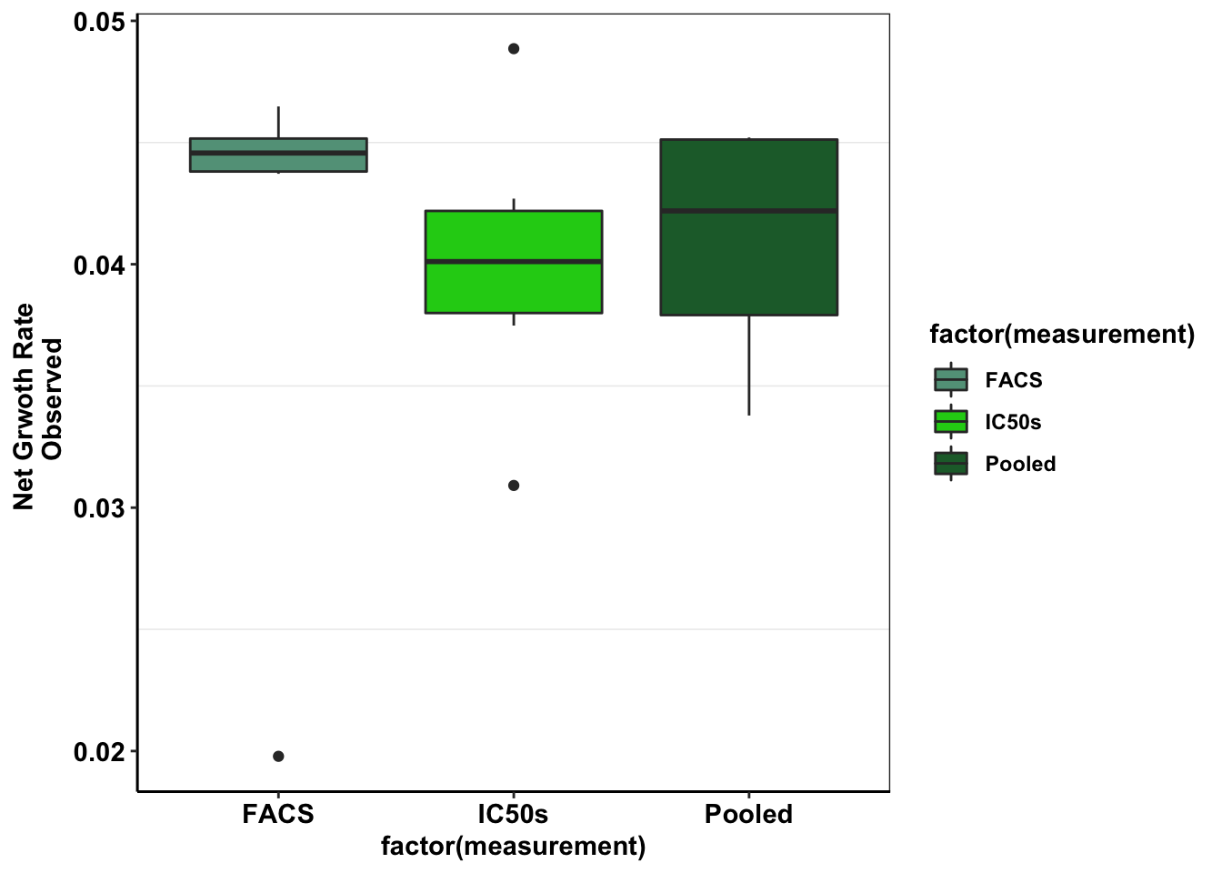

Past versions of unnamed-chunk-2-1.png

Version	Author	Date
4f82237	haiderinam	2020-06-02

ggplot(e255k_gr,aes(x=factor(measurement),y=netgr,fill=factor(measurement)))+
  geom_boxplot()+
  facet_wrap(~mutant)+
  scale_fill_manual(values = c("#63A088","#1CCE16","#206A36"))+
  scale_y_continuous(name="Net Grwoth Rate Observed")+
  cleanup+
  theme(legend.position = "none",
        axis.text.x=element_text(angle=15,hjust=.5,vjust=.5),
        axis.title.x=element_blank())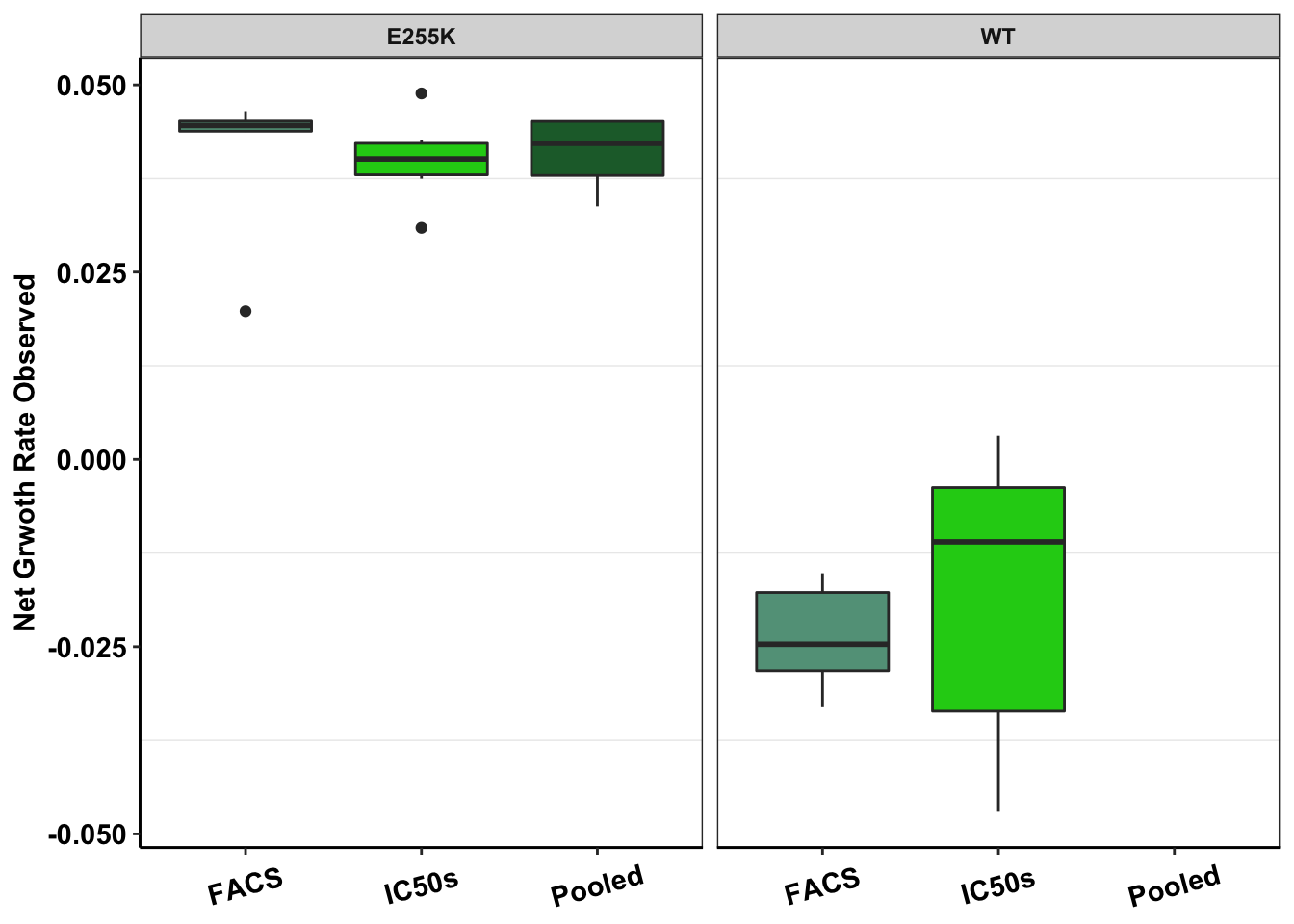

Past versions of unnamed-chunk-2-2.png

Version	Author	Date
4f82237	haiderinam	2020-06-02

# ggsave("e255k_wt_alphas_figure.pdf",width = 4,height = 3,units="in",useDingbats=F)

###Showing doubling Time###
ggplot(e255k_gr%>%filter(mutant=="E255K"),aes(x=factor(measurement),y=log(2)/netgr,fill=factor(measurement)))+geom_boxplot()+scale_fill_manual(values = c("#63A088","#1CCE16","#206A36"))+cleanup+scale_y_continuous(limits=c(0,30),name="Doubling Time")

Warning: Removed 1 rows containing non-finite values (stat_boxplot).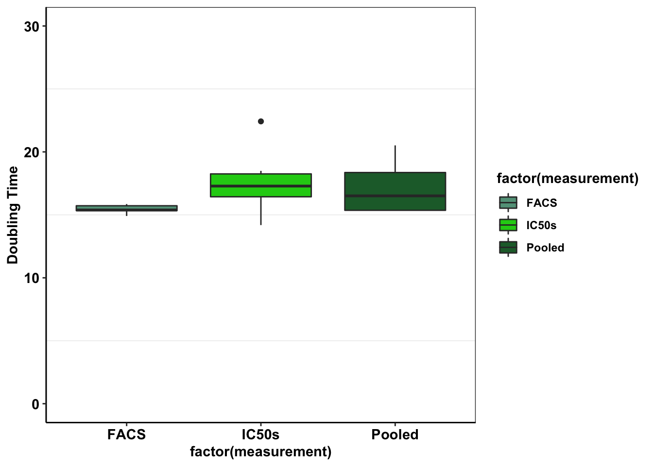

# Doubling time really spirals out of control with Wt because a proportion alive of .00001 is a 1000h doubling time.
# ggplot(e255k_gr,aes(x=factor(measurement),y=log(2)/netgr,fill=factor(measurement)))+geom_boxplot()+facet_wrap(~mutant)+scale_fill_manual(values = c("#63A088","#1CCE16","#206A36"))+cleanup+scale_y_continuous(limits=c(0,30),name="Doubling Time")
plotly=ggplot(e255k_gr[-c(38,29,16,14),],aes(x=factor(measurement),y=log(2)/netgr,fill=factor(measurement)))+geom_boxplot()+facet_wrap(~mutant)+scale_fill_manual(values = c("#63A088","#1CCE16","#206A36"))+cleanup
ggplotly(plotly)

#There seems to be a bit of a signal with the growth rates from D0 to D3 and D3 to D6. D0D3 seems to be a little higher. Will look at that discrepancy later.

gfpdata$ttotal_sequenced=c(0,3,6)
gfpdata$xtotal_sequenced=c(129,3323,37023)
# gfpdata_simple=gfpdata%>%dplyr::select(ttotal_4,xtotal_4_e255k)
# e255k=twinstrand_maf_merge%>%filter(mutant=="E255K",experiment=="M3")

ggplot(gfpdata)+
  geom_line(aes(x=t_out_4,y=x_out_4_e255k),color="#1cce16",size=1.5)+
  geom_ribbon(aes(x =t_out_4_conintub,ymax=x_out_4_e255k_ciub,ymin=x_out_4_e255k_cilb),fill="#1cce16",alpha=.3)+
  # geom_line(aes(x=t_out_3,y=log10(x_out_3_e255k)),color="#206A36",size=1.5)+
  # geom_ribbon(aes(x =t_out_3_conintub,ymax=log10(x_out_3_e255k_ciub),ymin=log10(x_out_3_e255k_cilb)),fill="#206A36",alpha=.3)+
  geom_point(aes(x=ttotal_4,y=xtotal_4_e255k),size=3)+
  # geom_point(aes(x=ttotal_3,y=xtotal_3_e255k),size=3)+
  geom_point(color="black",shape=21,size=3,aes(x=ttotal_sequenced,y=xtotal_sequenced,fill="orange"))+
  scale_x_continuous(name='Time (Days)',limits=c(0,7))+
  scale_y_continuous(trans="log10",name='Resistant Population',labels=parse(text = c("10^3","10^5")),breaks = c(10^3,10^5),limits=c(10^2,10^6))+
  theme_bw()+
  theme(plot.title = element_text(hjust=.5),
        legend.position="none",
        text = element_text(size=10),
        axis.text=element_text(face="bold",size="10",color="black"),
        axis.text.y =element_text(face="bold",size="10",color="black"),
        axis.title=element_text(face="bold",size="10",color="black"))

Warning: Removed 13 row(s) containing missing values (geom_path).

Warning: Removed 40 rows containing missing values (geom_point).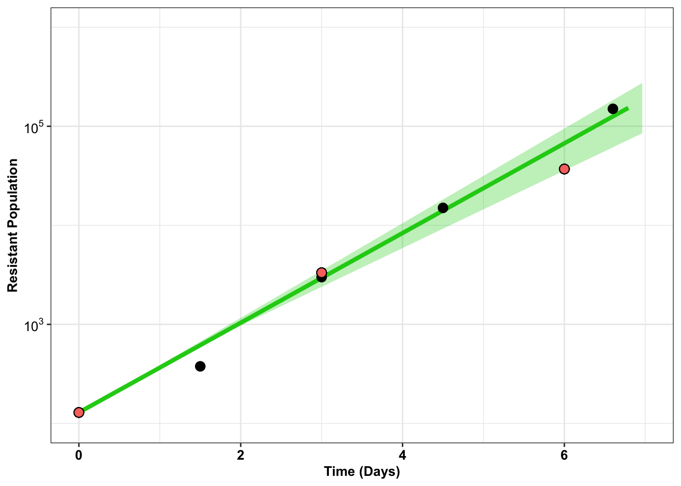

Past versions of unnamed-chunk-3-1.png

Version	Author	Date
4f82237	haiderinam	2020-06-02

  # scale_y_continuous(labels = function(x) format(x, scientific = TRUE), limits = c(1e2,5e6),trans='log10',labels=parse(text = c("10^3","10^5"))+
  # scale_y_continuous(labels = parse(text = c("10^3","10^5")), limits = c(1e2,5e6),trans='log10')+

# ggsave("e255k_initial_spikins_figure.pdf",width=3,height=3,units="in",useDingbats=F)

Looking at differences in growth rate between different replicates

#Fetching E255K growth rates that we saw in sequencing
e255k_sequenced=twinstrand_simple_melt_merge%>%filter(mutant%in%"E255K",duration%in%"d3d6")
e255k_sequenced_2=e255k_sequenced%>%mutate(measurement="Sequenced")%>%dplyr::select(Experiment=experiment,measurement,netgr_obs)
#Adding E255K growth rates that we saw during flow cytometry. These are the mean net growth rates from D3 to D6. Did not do D0 to D6 because we did not sequence D0 for all replicates and hence it would be an unfair comparison.
e255k_sequenced_facs=rbind(e255k_sequenced_2,
                 c("M3","FACs",0.035096215),
                 c("M4","FACs",0.028365649),
                 c("M5","FACs",0.016017951),
                 c("M6","FACs",0.02481819),
                 c("M7","FACs",0.026915217))

e255k_sequenced_facs$netgr_obs=as.numeric(as.character(e255k_sequenced_facs$netgr_obs))

#In the next step, I'm ordering mutants by decreasing resposne to the 625nM dose. Then I use this to change the levels of the species factor from more to less resistant. This helps with ggplot because now I can color the mutants with decreasing resistance
e255k_sequenced_facs$Experiment=factor(e255k_sequenced_facs$Experiment,levels = as.character(e255k_sequenced_facs$Experiment[order((e255k_sequenced_2$netgr_obs),decreasing = T)]))

ggplot(e255k_sequenced_facs,aes(x=Experiment,y=netgr_obs,fill=measurement))+
  geom_col(position="dodge")+
  scale_y_continuous(limits = c(0,NA))+
  scale_fill_manual(values=c("#1CCE16","#206A36"))+
  cleanup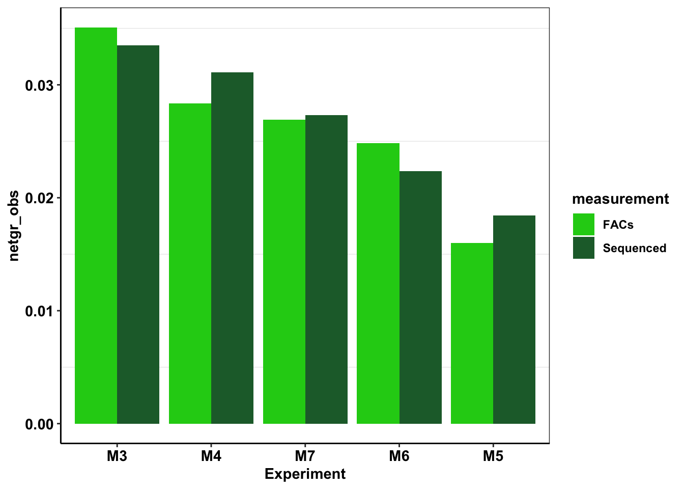

getPalette = colorRampPalette(brewer.pal(6, "Spectral"))
ggplot(e255k_sequenced_facs,aes(x=measurement,y=netgr_obs,group=Experiment))+
  geom_line()+
  geom_point(color="black",size=3,shape=21,aes(fill=Experiment))+
  cleanup+
  scale_y_continuous(name="Observed growth rate",limits = c(0,NA))+
  scale_fill_manual(values=getPalette(length(unique(e255k_sequenced_facs$Experiment))))+
  theme(axis.title.x = element_blank())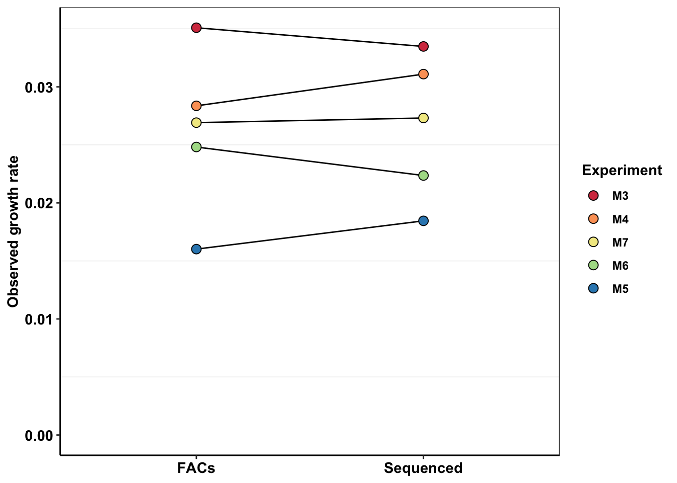

  # theme(axis.title.x = element_blank(),
        # legend.position = c(.9,.2))

# ggsave("e255k_facs_sequenced.pdf",width=4,height = 3,units = "in",useDingbats=F)

Looking at the growth rate changes with dates

a=twinstrand_simple_melt_merge%>%filter(duration%in%c("d0d3","d3d6"),experiment%in%c("M3","M6"))
plotly=ggplot(a,aes(x=factor(mutant),y=netgr_obs,fill=duration))+geom_col(position="dodge",stat="identity")+facet_wrap(~experiment)

Warning: Ignoring unknown parameters: stat

ggplotly(plotly)

#Realizing that the signal I'm seeing here might be confounded by erroneous flow cytometry counts... 

Session information

sessionInfo()

R version 4.0.0 (2020-04-24)
Platform: x86_64-apple-darwin17.0 (64-bit)
Running under: macOS Catalina 10.15.6

Matrix products: default
BLAS:   /Library/Frameworks/R.framework/Versions/4.0/Resources/lib/libRblas.dylib
LAPACK: /Library/Frameworks/R.framework/Versions/4.0/Resources/lib/libRlapack.dylib

locale:
[1] en_US.UTF-8/en_US.UTF-8/en_US.UTF-8/C/en_US.UTF-8/en_US.UTF-8

attached base packages:
[1] stats     graphics  grDevices utils     datasets  methods   base     

other attached packages:
 [1] RColorBrewer_1.1-2  reshape2_1.4.4      plotly_4.9.2.1     
 [4] dplyr_0.8.5         boot_1.3-24         lme4_1.1-23        
 [7] Matrix_1.2-18       fitdistrplus_1.0-14 npsurv_0.4-0.1     
[10] lsei_1.2-0.1        survival_3.1-12     MASS_7.3-51.5      
[13] ggplot2_3.3.0       lmtest_0.9-37       zoo_1.8-8          
[16] workflowr_1.6.2    

loaded via a namespace (and not attached):
 [1] statmod_1.4.34    tidyselect_1.1.0  xfun_0.13         purrr_0.3.4      
 [5] splines_4.0.0     lattice_0.20-41   colorspace_1.4-1  vctrs_0.3.0      
 [9] viridisLite_0.3.0 htmltools_0.4.0   yaml_2.2.1        rlang_0.4.6      
[13] later_1.0.0       pillar_1.4.4      nloptr_1.2.2.1    glue_1.4.1       
[17] withr_2.2.0       plyr_1.8.6        lifecycle_0.2.0   stringr_1.4.0    
[21] munsell_0.5.0     gtable_0.3.0      htmlwidgets_1.5.1 evaluate_0.14    
[25] labeling_0.3      knitr_1.28        crosstalk_1.1.0.1 httpuv_1.5.2     
[29] Rcpp_1.0.4.6      promises_1.1.0    scales_1.1.1      backports_1.1.7  
[33] jsonlite_1.6.1    farver_2.0.3      fs_1.4.1          digest_0.6.25    
[37] stringi_1.4.6     grid_4.0.0        rprojroot_1.3-2   tools_4.0.0      
[41] magrittr_1.5      lazyeval_0.2.2    tibble_3.0.1      tidyr_1.0.3      
[45] crayon_1.3.4      whisker_0.4       pkgconfig_2.0.3   ellipsis_0.3.1   
[49] data.table_1.12.8 httr_1.4.1        assertthat_0.2.1  minqa_1.2.4      
[53] rmarkdown_2.1     R6_2.4.1          nlme_3.1-147      git2r_0.27.1     
[57] compiler_4.0.0