Misc

workflowr

• Summary
• Checks
• Past versions

Last updated: 2020-06-07

Checks: 7 0

Knit directory: duplex_sequencing_screen/

This reproducible R Markdown analysis was created with workflowr (version 1.6.2). The Checks tab describes the reproducibility checks that were applied when the results were created. The Past versions tab lists the development history.

---

R Markdown file: up-to-date

Great! Since the R Markdown file has been committed to the Git repository, you know the exact version of the code that produced these results.

Environment: empty

Great job! The global environment was empty. Objects defined in the global environment can affect the analysis in your R Markdown file in unknown ways. For reproduciblity it’s best to always run the code in an empty environment.

Seed: set.seed(20200402)

The command set.seed(20200402) was run prior to running the code in the R Markdown file. Setting a seed ensures that any results that rely on randomness, e.g. subsampling or permutations, are reproducible.

Session information: recorded

Great job! Recording the operating system, R version, and package versions is critical for reproducibility.

Cache: none

Nice! There were no cached chunks for this analysis, so you can be confident that you successfully produced the results during this run.

File paths: relative

Great job! Using relative paths to the files within your workflowr project makes it easier to run your code on other machines.

Repository version: e2f801a

Great! You are using Git for version control. Tracking code development and connecting the code version to the results is critical for reproducibility.

The results in this page were generated with repository version e2f801a. See the Past versions tab to see a history of the changes made to the R Markdown and HTML files.

Note that you need to be careful to ensure that all relevant files for the analysis have been committed to Git prior to generating the results (you can use wflow_publish or wflow_git_commit). workflowr only checks the R Markdown file, but you know if there are other scripts or data files that it depends on. Below is the status of the Git repository when the results were generated:

Ignored files:
    Ignored:    .Rhistory
    Ignored:    .Rproj.user/

Untracked files:
    Untracked:  analysis/bcrabl_hill_ic50s.csv
    Untracked:  analysis/column_definitions_for_twinstrand_data_06062020.csv
    Untracked:  analysis/m351t_deviation.pdf
    Untracked:  analysis/multinomial_sims.Rmd
    Untracked:  analysis/pooled_growth_fig_cifrom4paramlogistic_060420.pdf
    Untracked:  analysis/pooled_growth_fig_cifromrawic50_060420.pdf
    Untracked:  analysis/simple_data_generation.Rmd
    Untracked:  analysis/twinstrand_growthrates_simple.csv
    Untracked:  analysis/twinstrand_maf_merge_simple.csv
    Untracked:  analysis/wildtype_growthrates_sequenced.csv
    Untracked:  clinicalabundancepredictions_BMES_abstract_51320.pdf
    Untracked:  data/Combined_data_frame_IC_Mutprob_abundance.csv
    Untracked:  data/IC50HeatMap.csv
    Untracked:  data/Twinstrand/
    Untracked:  data/gfpenrichmentdata.csv
    Untracked:  data/heatmap_concat_data.csv
    Untracked:  enrichment_simulations_3mutants.pdf
    Untracked:  output/archive/
    Untracked:  output/bmes_abstract_51220.pdf
    Untracked:  output/clinicalabundancepredictions_BMES_abstract_51320.pdf
    Untracked:  output/clinicalabundancepredictions_BMES_abstract_52020.pdf
    Untracked:  output/enrichment_simulations_3mutants_52020.pdf
    Untracked:  output/grant_fig.pdf
    Untracked:  output/grant_fig_v2.pdf
    Untracked:  output/grant_fig_v2updated.pdf
    Untracked:  output/ic50data_all_conc.csv
    Untracked:  shinyapp/

Unstaged changes:
    Modified:   analysis/E255K_alphas_figure.Rmd
    Modified:   analysis/clinical_abundance_predictions.Rmd
    Modified:   analysis/dosing_normalization.Rmd
    Modified:   analysis/index.Rmd
    Modified:   analysis/nonlinear_growth_analysis.Rmd
    Modified:   analysis/spikeins_depthofcoverages.Rmd
    Deleted:    data/README.md
    Modified:   output/twinstrand_maf_merge.csv
    Modified:   output/twinstrand_simple_melt_merge.csv

Note that any generated files, e.g. HTML, png, CSS, etc., are not included in this status report because it is ok for generated content to have uncommitted changes.

---

These are the previous versions of the repository in which changes were made to the R Markdown (analysis/misc.Rmd) and HTML (docs/misc.html) files. If you’ve configured a remote Git repository (see ?wflow_git_remote), click on the hyperlinks in the table below to view the files as they were in that past version.

File	Version	Author	Date	Message
Rmd	e2f801a	haiderinam	2020-06-07	wflow_publish(“analysis/misc.Rmd”)
html	eaca616	haiderinam	2020-04-20	Build site.
Rmd	2bba93e	haiderinam	2020-04-20	wflow_publish("analysis/*.Rmd")
html	c3e9499	haiderinam	2020-04-10	Build site.
Rmd	7a5e2ff	haiderinam	2020-04-10	wflow_publish(“analysis/misc.Rmd”)
html	e477777	haiderinam	2020-04-06	Build site.
Rmd	0a6e9cb	haiderinam	2020-04-06	wflow_publish(files = “analysis/misc.Rmd”)

---

Here I include some miscellaneous, pre-prod analyses

net_gr_wodrug=0.055
conc_for_predictions=0.8
########################Reading IC50 Data########################
ic50data_all=read.csv("data/IC50HeatMap.csv",header = T,stringsAsFactors = F)
# ic50data_all=read.csv("../data/IC50HeatMap.csv",header = T,stringsAsFactors = F)

twinstrand_maf_merge=read.csv("output/twinstrand_maf_merge.csv",header = T,stringsAsFactors = F)
# twinstrand_maf_merge=read.csv("../output/twinstrand_maf_merge.csv",header = T,stringsAsFactors = F)

# twinstrand_simple_melt_merge=read.csv("../output/twinstrand_simple_melt_merge.csv",header = T,stringsAsFactors = F)
twinstrand_simple_melt_merge=read.csv("output/twinstrand_simple_melt_merge.csv",header = T,stringsAsFactors = F)

# ic50data_long=read.csv("../output/ic50data_all_conc.csv",header = T,stringsAsFactors = F)
ic50data_long=read.csv("output/ic50data_all_conc.csv",header = T,stringsAsFactors = F)
ic50data_long$netgr_pred=net_gr_wodrug-ic50data_long$drug_effect

###Modeling out confidence intervals on growth rate predictions from IC50s Sources of error: 1. Sampling error (reads). Will be estimated by * Multinomial distributions based on observed coverages. * Sampling error in observed reads may be eliminated by removing mutants with <=1 depth of coverage

2. Dose response variability

• Well known observation that IC50s can vary by as much as 50%. Will incorporate this into predictions. One direct, albeit simple, solution is to just take the 95% confidence intervals of the IC50s that fell in the dose response range.

3. Dose variability. i.e. error between your expected dose and dose response.

Getting the dose responses for all mutants with the errors.

ic50data_all=ic50data_all%>%filter(species%in%c("Wt","V299L_H","E355A","D276G_maxi","H396R","F317L","F359I","E459K","G250E","F359C","F359V","M351T","L248V","E355G_maxi","Q252H_maxi","Y253F","F486S_maxi","H396P_maxi","E255K","Y253H","T315I","E255V"))


ic50data_all=ic50data_all%>%
  mutate(species=case_when(species=="F486S_maxi"~"F486S",
                          species=="H396P_maxi"~"H396P",
                          species=="Q252H_maxi"~"Q252H",
                          species=="E355G_maxi"~"E355G",
                          species=="D276G_maxi"~"D276G",
                          species=="V299L_H" ~ "V299L",
                          TRUE ~as.character(species)))


########################Getting Confidence Intervals########################
#will just start of with one dose at 1.25uM
ic50data_all2=data.frame(cbind(ic50data_all$species,ic50data_all$X1.25))
# ic50data_all2=data.frame(cbind(ic50data_all$species,ic50data_all$X0.625))
colnames(ic50data_all2)=c("species","dose_response")
ic50data_all2$dose_response=as.numeric(as.character(ic50data_all2$dose_response))


#Calculating confidence limit and standard deviations
ic50data_all_sum=ic50data_all2%>%group_by(species)%>%summarise(dr_mean=mean(dose_response),dr_ci_ul=dr_mean+1.96*sd(dose_response)*sqrt(n()),dr_ci_ll=dr_mean-1.96*sd(dose_response)*sqrt(n()),dr_sd_ul=dr_mean+sd(dose_response),dr_sd_ll=dr_mean-sd(dose_response))

#Since some mutants have 0% alive at the lower limit of the confidence interval, I'm converting those to 0
ic50data_all_sum=ic50data_all_sum%>%mutate(dr_ci_ll=case_when(dr_ci_ll<=0~0,
                                                              TRUE~dr_ci_ll),
                                           dr_sd_ll=case_when(dr_sd_ll<=0~0,
                                                              TRUE~dr_sd_ll))

#Dose response here is essentially y. aka %alive
#Converting y to drug effect on growth rate aka alpha value
ic50data_all_sum=ic50data_all_sum%>%mutate(netgr_pred_mean=net_gr_wodrug-(-log(dr_mean)/72),netgr_pred_ci_ul=net_gr_wodrug-(-log(dr_ci_ul)/72),netgr_pred_ci_ll=net_gr_wodrug-(-log(dr_ci_ll)/72),netgr_pred_sd_ul=net_gr_wodrug-(-log(dr_sd_ul)/72),netgr_pred_sd_ll=net_gr_wodrug-(-log(dr_sd_ll)/72))


########################Plotting Count with CIs########################
twinstrand_maf_merge=twinstrand_maf_merge%>%mutate(MAF=AltDepth/Depth)
twinstrand_maf_merge=merge(twinstrand_maf_merge%>%
                                 filter(experiment=="M3",tki_resistant_mutation=="True",!mutant%in%c("D276G",NA)),ic50data_all_sum%>%
                                 dplyr::select(species,netgr_pred_mean,netgr_pred_ci_ul,netgr_pred_ci_ll,netgr_pred_sd_ul,netgr_pred_sd_ll),by.x="mutant",by.y="species")

twinstrand_simple=twinstrand_maf_merge%>%dplyr::select(AltDepth,Depth,tki_resistant_mutation,mutant,experiment,Spike_in_freq,time_point,totalcells,totalmutant,MAF,netgr_pred_mean,netgr_pred_ci_ul,netgr_pred_ci_ll,netgr_pred_sd_ul,netgr_pred_sd_ll)

twinstrand_merge_forplot=melt(twinstrand_simple,id.vars = c("AltDepth","Depth","tki_resistant_mutation","mutant","experiment","Spike_in_freq","time_point","totalcells","netgr_pred_mean","netgr_pred_ci_ul","netgr_pred_ci_ll","netgr_pred_sd_ul","netgr_pred_sd_ll"),variable.name = "count_type",value.name = "count")
# twinstrand_merge_forplot=merge(twinstrand_maf_merge%>%filter(experiment=="M3",tki_resistant_mutation=="True",!mutant%in%c("D276G",NA)),ic50data_all_sum%>%dplyr::select(species,netgr_pred_mean,netgr_pred_ci_ul,netgr_pred_ci_ll,netgr_pred_sd_ul,netgr_pred_sd_ll),by.x="mutant",by.y="species")

#Basically making an extra column with the D0 total mutant counts for each mutant
twinstrand_merge_forplot=merge(twinstrand_merge_forplot,twinstrand_merge_forplot%>%filter(time_point=="D0")%>%dplyr::select(mutant,count_type,count_D0=count),by=c("mutant","count_type"))
    #########Here, figure out why twinstrand_merge_forplot is having two rows for each mutant after being merged with a D0 version of itself. This is leading to weird plotting artifacts
    
    # a=twinstrand_merge_forplot%>%filter(count_type=="totalmutant",mutant=="E255K",time_point=="D0")
    ############

twinstrand_merge_forplot=twinstrand_merge_forplot%>%mutate(time=case_when(time_point=="D0"~0,
                            time_point=="D3"~72,
                            time_point=="D6"~144),
                           ci_mean=count_D0*exp(netgr_pred_mean*time),
                           ci_ul=count_D0*exp(netgr_pred_ci_ul*time),
                           ci_ll=count_D0*exp(netgr_pred_ci_ll*time),
                           sd_ul=count_D0*exp(netgr_pred_sd_ul*time),
                           sd_ll=count_D0*exp(netgr_pred_sd_ll*time))
twinstrand_merge_forplot=twinstrand_merge_forplot%>%mutate(ci_ll=case_when(ci_ll=="NaN"~0,
                                           TRUE~ci_ll))

####Since the more sensitive mutants were appearing to grow fast if I take the raw IC50 predicted growth rates, I am going to instead take the predicted growth rates from the IC50s that were fit on a 4-parameter logistic. To get standard deviations, I will just add/subtract the standard deviations from the regular plots.
twinstrand_merge_forplot=merge(twinstrand_merge_forplot,ic50data_long%>%filter(conc==conc_for_predictions)%>%dplyr::select(mutant,netgr_pred_model=netgr_pred),by = "mutant")
twinstrand_merge_forplot=twinstrand_merge_forplot%>%mutate(netgr_pred_model_sd_ul=netgr_pred_model+(netgr_pred_mean-netgr_pred_sd_ll),netgr_pred_model_sd_ll=netgr_pred_model-(netgr_pred_mean-netgr_pred_sd_ll))

twinstrand_merge_forplot=twinstrand_merge_forplot%>%mutate(
                           sd_mean_model=count_D0*exp(netgr_pred_model*time),
                           sd_ul_model=count_D0*exp(netgr_pred_model_sd_ul*time),
                           sd_ll_model=count_D0*exp(netgr_pred_model_sd_ll*time))
twinstrand_merge_forplot=twinstrand_merge_forplot%>%mutate(ci_ll=case_when(ci_ll=="NaN"~0,
                                           TRUE~ci_ll))
###########

#Factoring the mutants from more to less resistant
twinstrand_merge_forplot$mutant=factor(twinstrand_merge_forplot$mutant,levels = as.character(unique(twinstrand_merge_forplot$mutant[order((twinstrand_merge_forplot$netgr_pred_mean),decreasing = T)])))



getPalette = colorRampPalette(brewer.pal(9, "Spectral"))
####In the plots below, the dashed line is the mean prediction form the IC50s. Points are what we see in the spike-in experiment

#Plotting with 95% confidence intervals
# %>%filter(count_type=="totalmutant")
ggplot(twinstrand_merge_forplot,aes(x=time/24,y=count,fill=factor(mutant)))+geom_point()+
  facet_grid(count_type~mutant)+
  geom_line(aes(y=ci_mean),linetype="dashed")+
  geom_ribbon(aes(ymin=ci_ll,ymax=ci_ul,alpha=.3))+
  scale_y_continuous(trans="log2")+
  cleanup+
  scale_fill_manual(values = getPalette(length(unique(twinstrand_merge_forplot$mutant))))

Warning: Transformation introduced infinite values in continuous y-axis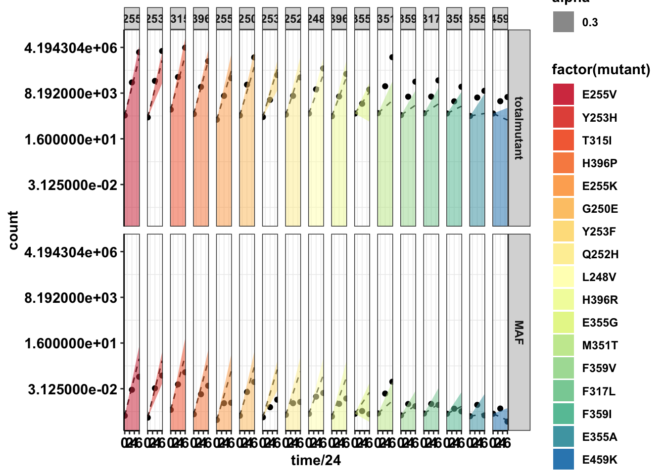

Past versions of unnamed-chunk-3-1.png

Version	Author	Date
c3e9499	haiderinam	2020-04-10

#Plotting with standard deviations
ggplot(twinstrand_merge_forplot,aes(x=time/24,y=count,fill=factor(mutant),shape=factor(count_type)))+geom_point()+
  geom_line(aes(y=ci_mean),linetype="dashed")+
  geom_ribbon(aes(ymin=sd_ll,ymax=sd_ul,alpha=.3))+
  facet_wrap(~mutant,ncol=4)+
  scale_y_continuous(trans="log2")+
  cleanup+
  scale_fill_manual(values = getPalette(length(unique(twinstrand_merge_forplot$mutant))))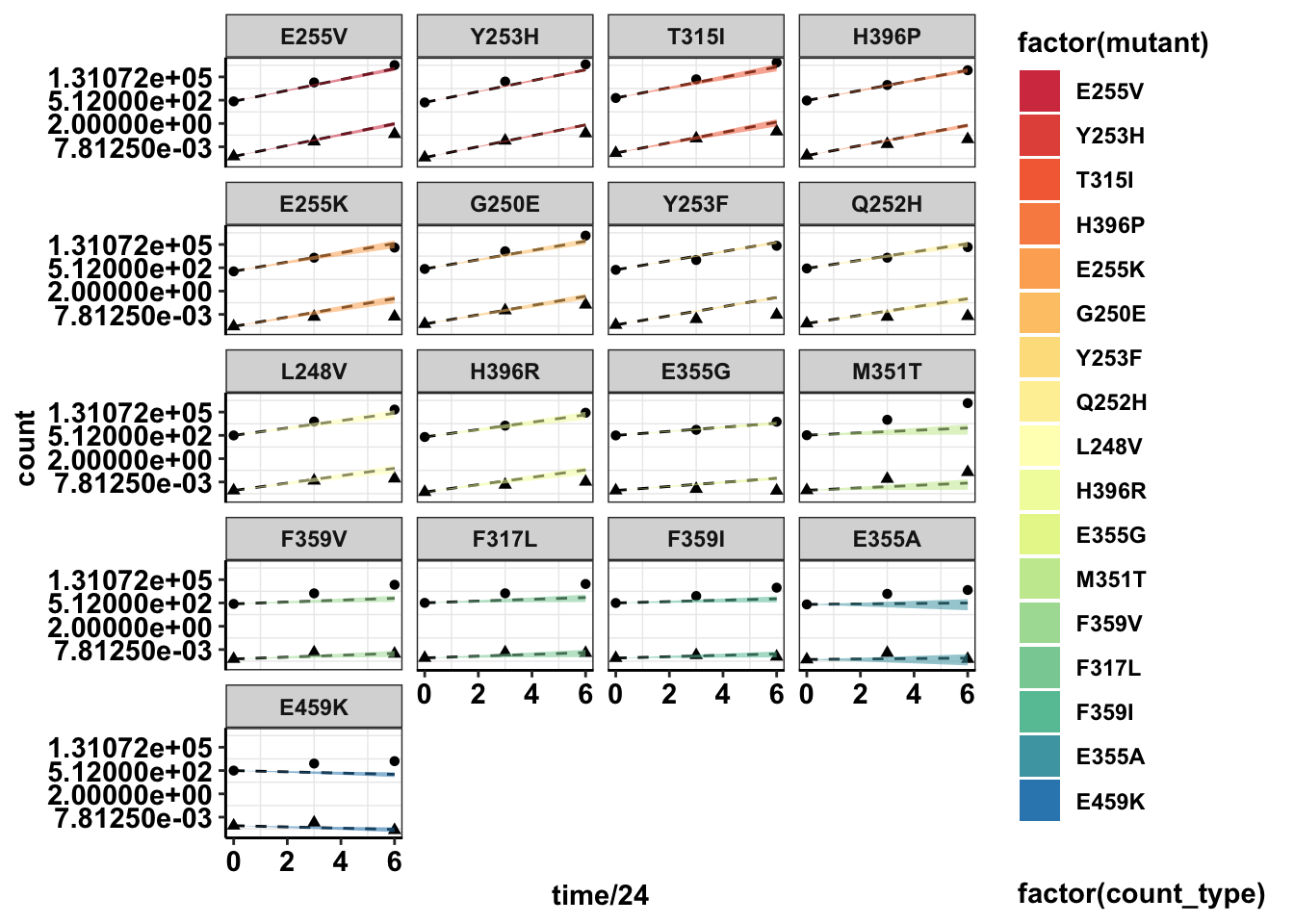

Past versions of unnamed-chunk-3-2.png

Version	Author	Date
c3e9499	haiderinam	2020-04-10

#Next step: extend for experiments besides M3

plotly=ggplot(twinstrand_merge_forplot%>%filter(count_type=="totalmutant"),aes(x=time/24,y=count,fill=factor(mutant),shape=factor(count_type)))+geom_point()+
  geom_line(aes(y=ci_mean),linetype="dashed")+
  geom_ribbon(aes(ymin=sd_ll,ymax=sd_ul,alpha=.3))+
  facet_wrap(~mutant,ncol=4)+
  scale_y_continuous(trans="log2")+
  cleanup+
  scale_fill_manual(values = getPalette(length(unique(twinstrand_merge_forplot$mutant))))
ggplotly(plotly)

plotly=ggplot(twinstrand_merge_forplot%>%filter(count_type=="MAF"),aes(x=time/24,y=count,fill=factor(mutant),shape=factor(count_type)))+geom_point()+
  geom_line(aes(y=ci_mean),linetype="dashed")+
  geom_ribbon(aes(ymin=sd_ll,ymax=sd_ul,alpha=.3))+
  facet_wrap(~mutant,ncol=4)+
  scale_y_continuous(trans="log2")+
  cleanup+
  scale_fill_manual(values = getPalette(length(unique(twinstrand_merge_forplot$mutant))))
ggplotly(plotly)

#Plotting IC50s form 4 Parameter model
plotly=ggplot(twinstrand_merge_forplot%>%filter(count_type=="totalmutant"),aes(x=time/24,y=count,fill=factor(mutant),shape=factor(count_type)))+geom_point()+
  geom_line(aes(y=sd_mean_model),linetype="dashed")+
  geom_ribbon(aes(ymin=sd_ll_model,ymax=sd_ul_model,alpha=.3))+
  facet_wrap(~mutant,ncol=4)+
  scale_y_continuous(trans="log2")+
  cleanup+
  scale_fill_manual(values = getPalette(length(unique(twinstrand_merge_forplot$mutant))))
ggplotly(plotly)

plotly=ggplot(twinstrand_merge_forplot%>%filter(count_type=="MAF"),aes(x=time/24,y=count,fill=factor(mutant),shape=factor(count_type)))+geom_point()+
  geom_line(aes(y=sd_mean_model),linetype="dashed")+
  geom_ribbon(aes(ymin=sd_ll_model,ymax=sd_ul_model,alpha=.3))+
  facet_wrap(~mutant,ncol=4)+
  scale_y_continuous(trans="log2")+
  cleanup+
  scale_fill_manual(values = getPalette(length(unique(twinstrand_merge_forplot$mutant))))
ggplotly(plotly)

#51220
#Adding all experiments, and not just M3

This is the exact same as the chunk above except that it has been modified to make error bars across experiments

twinstrand_maf_merge=read.csv("output/twinstrand_maf_merge.csv",header = T,stringsAsFactors = F)
# twinstrand_maf_merge=read.csv("../output/twinstrand_maf_merge.csv",header = T,stringsAsFactors = F)

ic50data_all=read.csv("data/IC50HeatMap.csv",header = T,stringsAsFactors = F)
# ic50data_all=read.csv("../data/IC50HeatMap.csv",header = T,stringsAsFactors = F)

ic50data_all=ic50data_all%>%filter(species%in%c("Wt","V299L_H","E355A","D276G_maxi","H396R","F317L","F359I","E459K","G250E","F359C","F359V","M351T","L248V","E355G_maxi","Q252H_maxi","Y253F","F486S_maxi","H396P_maxi","E255K","Y253H","T315I","E255V"))


ic50data_all=ic50data_all%>%
  mutate(species=case_when(species=="F486S_maxi"~"F486S",
                          species=="H396P_maxi"~"H396P",
                          species=="Q252H_maxi"~"Q252H",
                          species=="E355G_maxi"~"E355G",
                          species=="D276G_maxi"~"D276G",
                          species=="V299L_H" ~ "V299L",
                          TRUE ~as.character(species)))


########################Getting Confidence Intervals########################
#will just start of with one dose at 1.25uM
ic50data_all2=data.frame(cbind(ic50data_all$species,ic50data_all$X1.25))
# ic50data_all2=data.frame(cbind(ic50data_all$species,ic50data_all$X0.625))
colnames(ic50data_all2)=c("species","dose_response")
ic50data_all2$dose_response=as.numeric(as.character(ic50data_all2$dose_response))


#Calculating confidence limit and standard deviations
ic50data_all_sum=ic50data_all2%>%group_by(species)%>%summarise(dr_mean=mean(dose_response),dr_ci_ul=dr_mean+1.96*sd(dose_response)*sqrt(n()),dr_ci_ll=dr_mean-1.96*sd(dose_response)*sqrt(n()),dr_sd_ul=dr_mean+sd(dose_response),dr_sd_ll=dr_mean-sd(dose_response))

#Since some mutants have 0% alive at the lower limit of the confidence interval, I'm converting those to 0
ic50data_all_sum=ic50data_all_sum%>%mutate(dr_ci_ll=case_when(dr_ci_ll<=0~0,
                                                              TRUE~dr_ci_ll),
                                           dr_sd_ll=case_when(dr_sd_ll<=0~0,
                                                              TRUE~dr_sd_ll))

#Dose response here is essentially y. aka %alive
#Converting y to drug effect on growth rate aka alpha value
ic50data_all_sum=ic50data_all_sum%>%mutate(netgr_pred_mean=net_gr_wodrug-(-log(dr_mean)/72),netgr_pred_ci_ul=net_gr_wodrug-(-log(dr_ci_ul)/72),netgr_pred_ci_ll=net_gr_wodrug-(-log(dr_ci_ll)/72),netgr_pred_sd_ul=net_gr_wodrug-(-log(dr_sd_ul)/72),netgr_pred_sd_ll=net_gr_wodrug-(-log(dr_sd_ll)/72))


#First, creating day 0 values for M4,M5,M7, and sp_enu_3. Whenever you see any of these experiments, add M3's or M6's or Sp_Enu4's D0 counts for its counts.
M3D0=twinstrand_maf_merge%>%filter(experiment=="M3",time_point=="D0")
M5D0=M3D0%>%mutate(experiment="M5")
M7D0=M3D0%>%mutate(experiment="M7")
M6D0=twinstrand_maf_merge%>%filter(experiment=="M6",time_point=="D0")
M4D0=M6D0%>%mutate(experiment="M4")
Enu3_D0=twinstrand_maf_merge%>%filter(experiment=="Enu_3",time_point=="D0")
Enu4_D0=Enu3_D0%>%mutate(experiment="Enu_4")
twinstrand_maf_merge=rbind(twinstrand_maf_merge,M5D0,M7D0,M4D0,Enu4_D0)
########################Plotting Count with CIs########################
twinstrand_maf_merge=twinstrand_maf_merge%>%filter(experiment%in%c("M3","M5","M7"))%>%mutate(MAF=AltDepth/Depth)
twinstrand_maf_merge=merge(twinstrand_maf_merge%>%
                                 filter(tki_resistant_mutation=="True",!mutant%in%c("D276G",NA)),ic50data_all_sum%>%
                                 dplyr::select(species,netgr_pred_mean,netgr_pred_ci_ul,netgr_pred_ci_ll,netgr_pred_sd_ul,netgr_pred_sd_ll),by.x="mutant",by.y="species")

twinstrand_simple=twinstrand_maf_merge%>%dplyr::select(AltDepth,Depth,tki_resistant_mutation,mutant,experiment,Spike_in_freq,time_point,totalcells,totalmutant,MAF,netgr_pred_mean,netgr_pred_ci_ul,netgr_pred_ci_ll,netgr_pred_sd_ul,netgr_pred_sd_ll)

twinstrand_merge_forplot=melt(twinstrand_simple,id.vars = c("AltDepth","Depth","tki_resistant_mutation","mutant","experiment","Spike_in_freq","time_point","totalcells","netgr_pred_mean","netgr_pred_ci_ul","netgr_pred_ci_ll","netgr_pred_sd_ul","netgr_pred_sd_ll"),variable.name = "count_type",value.name = "count")
# twinstrand_merge_forplot=merge(twinstrand_maf_merge%>%filter(experiment=="M3",tki_resistant_mutation=="True",!mutant%in%c("D276G",NA)),ic50data_all_sum%>%dplyr::select(species,netgr_pred_mean,netgr_pred_ci_ul,netgr_pred_ci_ll,netgr_pred_sd_ul,netgr_pred_sd_ll),by.x="mutant",by.y="species")

#Basically making an extra column with the D0 total mutant counts for each mutant

twinstrand_merge_forplot=merge(twinstrand_merge_forplot,twinstrand_merge_forplot%>%filter(time_point=="D0")%>%dplyr::select(mutant,count_type,experiment,count_D0=count),by=c("mutant","count_type","experiment"))
    #########Here, figure out why twinstrand_merge_forplot is having two rows for each mutant after being merged with a D0 version of itself. This is leading to weird plotting artifacts
    
    # a=twinstrand_merge_forplot%>%filter(count_type=="totalmutant",mutant=="E255K",time_point=="D0")
    ############

twinstrand_merge_forplot=twinstrand_merge_forplot%>%mutate(time=case_when(time_point=="D0"~0,
                            time_point=="D3"~72,
                            time_point=="D6"~144),
                           ci_mean=count_D0*exp(netgr_pred_mean*time),
                           ci_ul=count_D0*exp(netgr_pred_ci_ul*time),
                           ci_ll=count_D0*exp(netgr_pred_ci_ll*time),
                           sd_ul=count_D0*exp(netgr_pred_sd_ul*time),
                           sd_ll=count_D0*exp(netgr_pred_sd_ll*time))
twinstrand_merge_forplot=twinstrand_merge_forplot%>%mutate(ci_ll=case_when(ci_ll=="NaN"~0,
                                           TRUE~ci_ll))

####Since the more sensitive mutants were appearing to grow fast if I take the raw IC50 predicted growth rates, I am going to instead take the predicted growth rates from the IC50s that were fit on a 4-parameter logistic. To get standard deviations, I will just add/subtract the standard deviations from the regular plots.
twinstrand_merge_forplot=merge(twinstrand_merge_forplot,ic50data_long%>%filter(conc==conc_for_predictions)%>%dplyr::select(mutant,netgr_pred_model=netgr_pred),by = "mutant")
twinstrand_merge_forplot=twinstrand_merge_forplot%>%mutate(netgr_pred_model_sd_ul=netgr_pred_model+(netgr_pred_mean-netgr_pred_sd_ll),netgr_pred_model_sd_ll=netgr_pred_model-(netgr_pred_mean-netgr_pred_sd_ll))

twinstrand_merge_forplot=twinstrand_merge_forplot%>%mutate(
                           sd_mean_model=count_D0*exp(netgr_pred_model*time),
                           sd_ul_model=count_D0*exp(netgr_pred_model_sd_ul*time),
                           sd_ll_model=count_D0*exp(netgr_pred_model_sd_ll*time))
twinstrand_merge_forplot=twinstrand_merge_forplot%>%mutate(ci_ll=case_when(ci_ll=="NaN"~0,
                                           TRUE~ci_ll))
###########

#Factoring the mutants from more to less resistant
twinstrand_merge_forplot$mutant=factor(twinstrand_merge_forplot$mutant,levels = as.character(unique(twinstrand_merge_forplot$mutant[order((twinstrand_merge_forplot$netgr_pred_mean),decreasing = T)])))



getPalette = colorRampPalette(brewer.pal(9, "Spectral"))
####In the plots below, the dashed line is the mean prediction form the IC50s. Points are what we see in the spike-in experiment


#Plotting IC50s form 4 Parameter model
plotly=ggplot(twinstrand_merge_forplot%>%filter(count_type=="totalmutant"),aes(x=time/24,y=count,fill=factor(mutant),shape=factor(count_type)))+geom_point()+
  geom_line(aes(y=sd_mean_model),linetype="dashed")+
  geom_ribbon(aes(ymin=sd_ll_model,ymax=sd_ul_model,alpha=.3))+
  facet_wrap(~mutant,ncol=4)+
  scale_y_continuous(trans="log2")+
  cleanup+
  scale_fill_manual(values = getPalette(length(unique(twinstrand_merge_forplot$mutant))))
ggplotly(plotly)

plotly=ggplot(twinstrand_merge_forplot%>%filter(count_type=="MAF"),aes(x=time/24,y=count,fill=factor(mutant),shape=factor(count_type)))+geom_point()+
  geom_line(aes(y=sd_mean_model),linetype="dashed")+
  geom_ribbon(aes(ymin=sd_ll_model,ymax=sd_ul_model,alpha=.3))+
  facet_wrap(~mutant,ncol=4)+
  scale_y_continuous(trans="log2")+
  cleanup+
  scale_fill_manual(values = getPalette(length(unique(twinstrand_merge_forplot$mutant))))
ggplotly(plotly)

plotly=ggplot(twinstrand_merge_forplot%>%filter(mutant%in%"T315I",count_type=="totalmutant"),aes(x=time/24,y=count,fill=factor(mutant),shape=factor(count_type)))+geom_boxplot()+
  geom_line(aes(y=sd_mean_model),linetype="dashed")+
  geom_ribbon(aes(ymin=sd_ll_model,ymax=sd_ul_model,alpha=.3))+
  facet_wrap(~mutant,ncol=4)+
  scale_y_continuous(trans="log2")+
  cleanup+
  scale_fill_manual(values = getPalette(length(unique(twinstrand_merge_forplot$mutant))))
ggplotly(plotly)

#Calculating errors in observed datapoints.
twinstrand_merge_forplot_means=twinstrand_merge_forplot%>%group_by(mutant,count_type,time_point)%>%summarize(time=mean(time),count_mean_obs=mean(count),count_sd_obs=sd(count),sd_mean_model=mean(sd_mean_model),sd_ll_model=mean(sd_ll_model),sd_ul_model=mean(sd_ul_model))

ggplot(twinstrand_merge_forplot_means%>%filter(!mutant%in%c("E459K"),count_type%in%"totalmutant"),aes(x=time/24,y=count_mean_obs,fill=factor(mutant)))+
  geom_point(size=.5)+
  # geom_point(aes(color=factor(mutant),size=.1))+
  geom_errorbar(aes(ymin=count_mean_obs-count_sd_obs,ymax=count_mean_obs+count_sd_obs),width=.7)+
  facet_wrap(~mutant,ncol=4)+
  cleanup+
  scale_y_continuous(trans="log10",name="Count",breaks=c(1e2,1e4,1e6),labels=parse(text=c("10^2","10^4","10^6")))+
  scale_x_discrete(name="Time (Days)",breaks=c(0,3,6),limits=c(1,1000000))+
  theme(legend.position = "none")+
  geom_line(aes(y=sd_mean_model),linetype="dashed")+
  geom_ribbon(aes(ymin=sd_ll_model,ymax=sd_ul_model,alpha=.3))+
  scale_fill_manual(values = getPalette(length(unique(twinstrand_merge_forplot$mutant))))+
  scale_color_manual(values = getPalette(length(unique(twinstrand_merge_forplot$mutant))))+
  theme(strip.text=element_blank(),
        axis.title.x = element_blank(),
        axis.title.y = element_blank())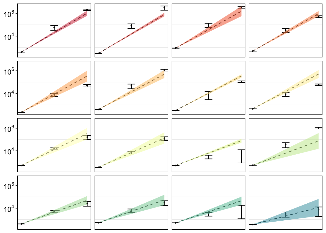

  # theme(strip.text=element_text(size=6,face="bold"),strip.background = element_rect(fill="white"))
# ggplotly(plotly)
# ggsave("bmes_abstract_51220.pdf",width=2,height=2,units="in",useDingbats=F)
ggsave("pooled_growth_fig_cifromrawic50_060420.pdf",width=3,height=3,units="in",useDingbats=F)

# a=twinstrand_merge_forplot%>%filter(mutant=="F359I")
# b=a%>%filter(mutant=="F359I",count_type=="totalmutant",time_point=="D6")

#Problem now is that there is a lot of variation across experiments because of the different spike-in frequencies used and because of the random differences in Depth. This means that it doesn't really make sense to do error bars unless you normalize all experiments to start at a relative count of 1. So I am having to normalize to get a relative count of 1. Or not use the errorbars at all. I eventually ended up using only counts from M3


ggplot(twinstrand_merge_forplot_means%>%filter(mutant%in%c("T315I","L248V","E355A","F317L"),count_type%in%"totalmutant"),aes(x=time/24,y=count_mean_obs,fill=factor(mutant)))+
  geom_point(size=.5)+
  # geom_point(aes(color=factor(mutant),size=.1))+
  geom_errorbar(aes(ymin=count_mean_obs-count_sd_obs,ymax=count_mean_obs+count_sd_obs),width=.7)+
  facet_wrap(~mutant)+
  cleanup+
  scale_y_continuous(trans="log10",name="Count",breaks=c(1e2,1e4,1e6),labels=parse(text=c("10^2","10^4","10^6")))+
  scale_x_discrete(name="Time (Days)",breaks=c(0,3,6),limits=c(1,1000000))+
  theme(legend.position = "none")+
  geom_line(aes(y=sd_mean_model),linetype="dashed")+
  geom_ribbon(aes(ymin=sd_ll_model,ymax=sd_ul_model,alpha=.3))+
  scale_fill_manual(values = getPalette(length(unique(twinstrand_merge_forplot$mutant))))+
  scale_color_manual(values = getPalette(length(unique(twinstrand_merge_forplot$mutant))))+
  theme(strip.text=element_blank(),
        axis.title.x = element_blank(),
        axis.title.y = element_blank())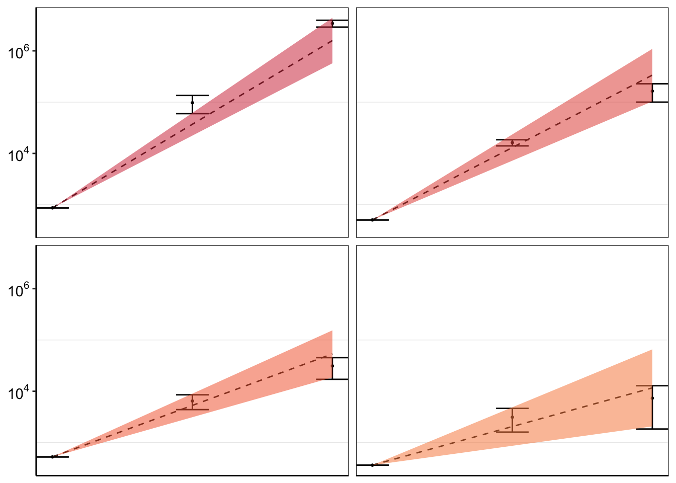

# ggplotly(plotly)

###########################Plotting Deviation from expectations for all mutants####################################

############D3############
deviations=twinstrand_merge_forplot_means%>%filter(time_point=="D3",count_type=="totalmutant")
ggplot(deviations,aes(x=mutant,y=(count_mean_obs-sd_mean_model)*100/sd_mean_model,color=mutant,label=mutant))+geom_text()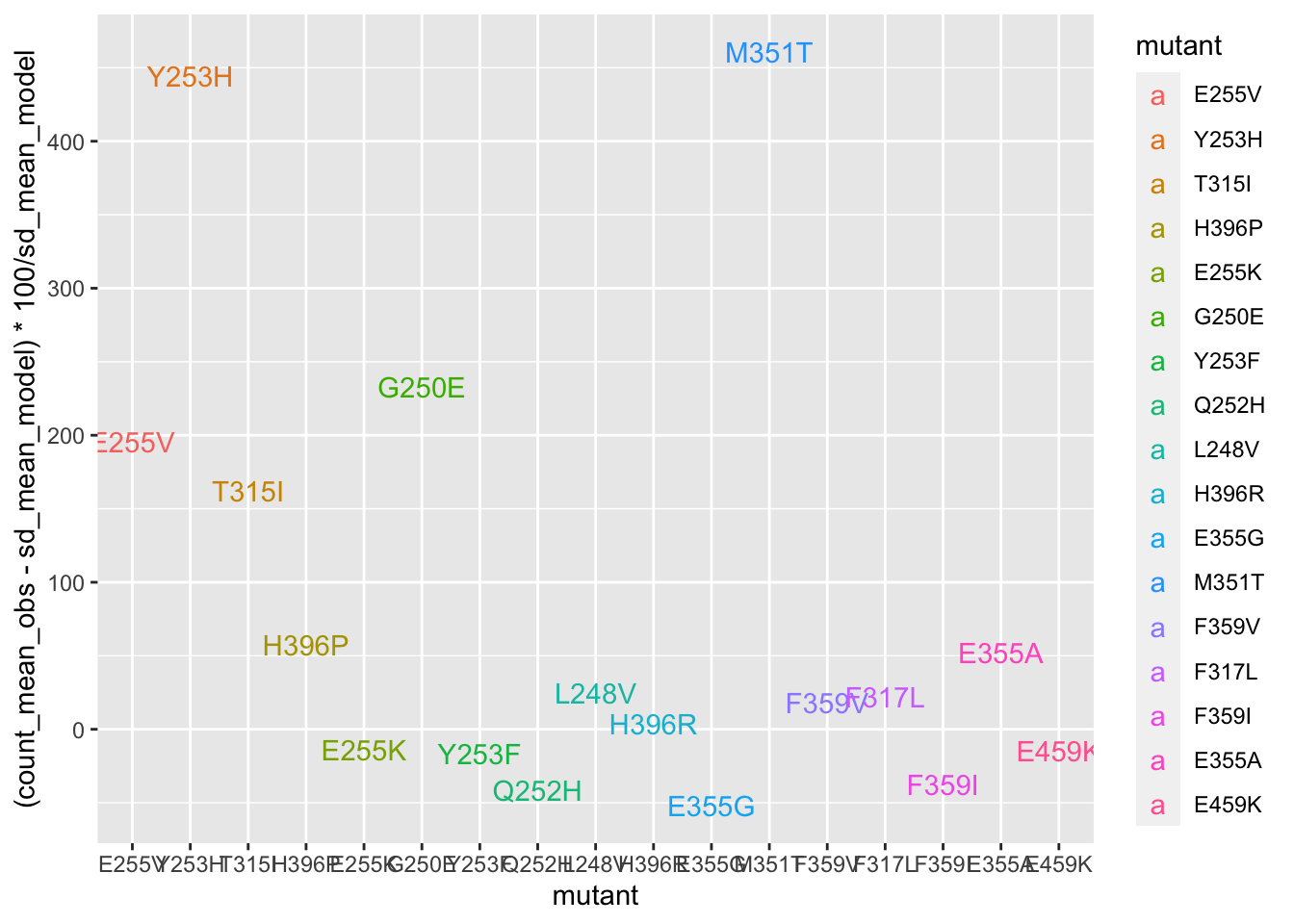

#####Plotting it in a hazard ratio fashion. Wheras the other plots show %increase in counts vs expectations, this hazard ratio plot also helps hone in on some of the mutants that got decreased by a lot. In a sense, it is a fairer plot.
ggplot(deviations,aes(y=mutant,x=(count_mean_obs/sd_mean_model),color=mutant,label=mutant))+geom_text()+scale_x_continuous(trans="log10")+geom_vline(aes(xintercept=1))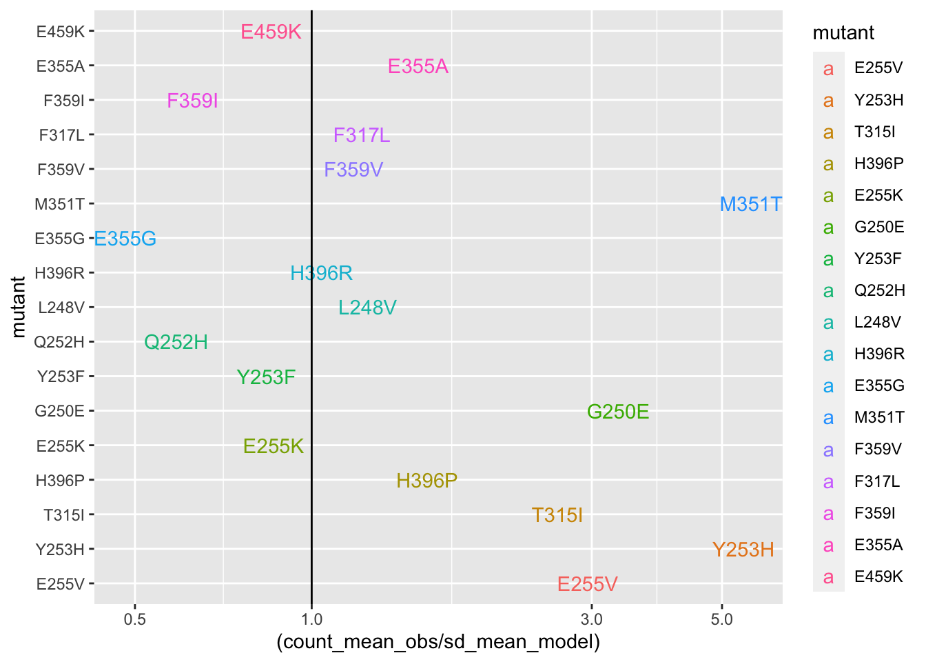

ggplot(deviations,aes(x=mutant,y=(count_mean_obs-sd_mean_model)*100/sd_mean_model,fill=mutant))+geom_col()+cleanup+theme(legend.position = "none")+scale_y_continuous(name=" % Difference between observed and expected cell counts")+scale_fill_manual(values = getPalette(length(unique(twinstrand_merge_forplot$mutant))))+
  scale_color_manual(values = getPalette(length(unique(twinstrand_merge_forplot$mutant))))+
  theme(axis.title.x = element_blank())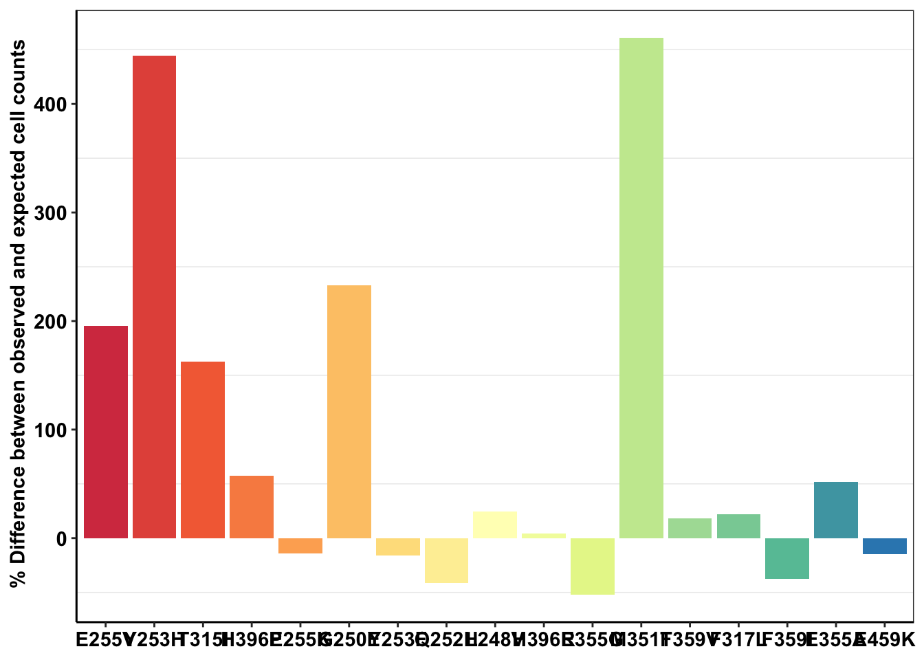

############D6############
deviations=twinstrand_merge_forplot_means%>%filter(time_point=="D6",count_type=="totalmutant")
ggplot(deviations,aes(x=mutant,y=(count_mean_obs-sd_mean_model)*100/sd_mean_model,color=mutant,label=mutant))+geom_text()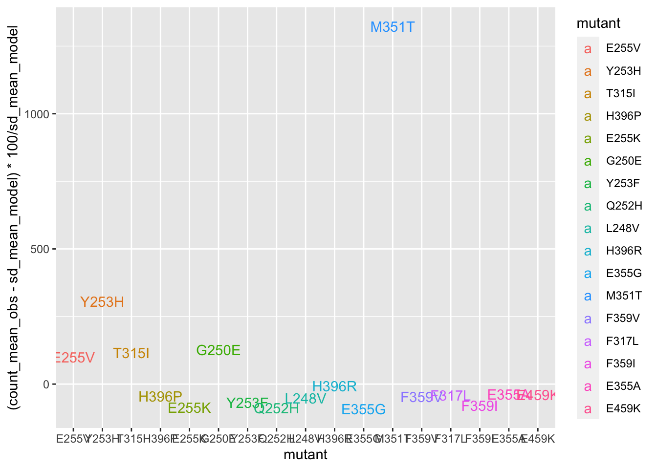

ggplot(deviations,aes(x=mutant,y=(count_mean_obs-sd_mean_model)*100/sd_mean_model,fill=mutant))+geom_col()+cleanup+theme(legend.position = "none")+scale_y_continuous(name=" % Difference between observed \n and expected cell counts")+scale_fill_manual(values = getPalette(length(unique(twinstrand_merge_forplot$mutant))))+
  scale_color_manual(values = getPalette(length(unique(twinstrand_merge_forplot$mutant))))+
  theme(axis.title.x = element_blank(),
        axis.text.x=element_text(angle=90,hjust=.5,vjust=.5))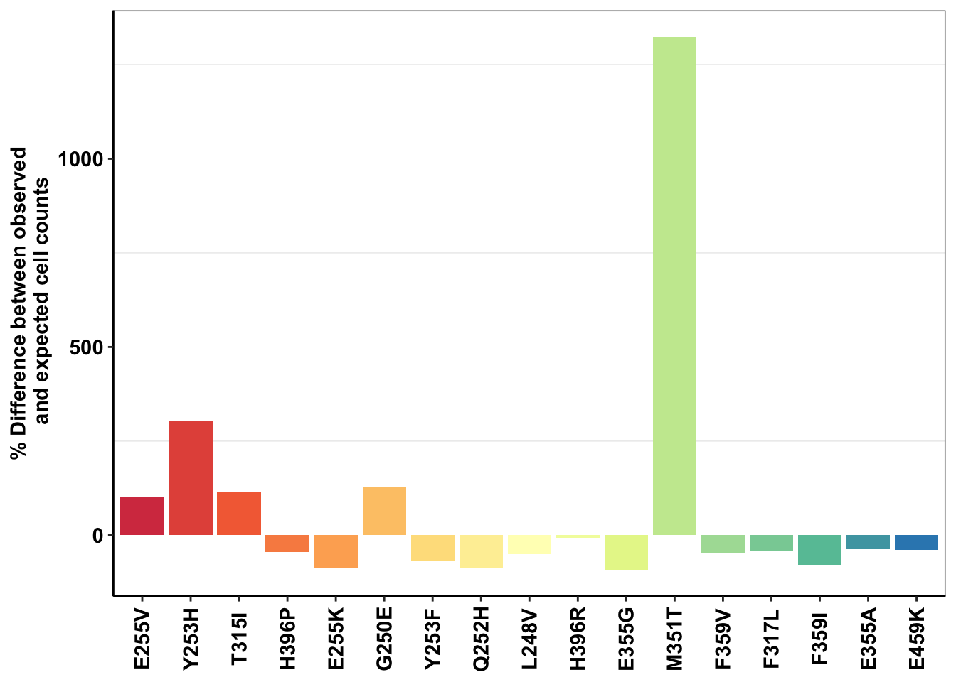

ggsave("m351t_deviation.pdf",width=4,height = 2,units="in",useDingbats=F)
 
###Things that I would like to do to see if this huge M351T deviation from expectations is real: 1) Right now, you were only looking at M3, M5, M7. Look at M4, M6 too. Maybe make a boxplot with errorbars. 2) You were only looking at the %age deviation of observed vs predicted counts at D3, D6 etc. Look at %age deviation in *netgrowthrate* between observed and predicted.

Plotting Shendure’s observed vs predicted plots

###Not evalutating this chunk because it's throwing an interesting error
a_sum=twinstrand_merge_forplot%>%group_by(mutant,count_type)%>%summarize(netgr_obs=log(count[time_point=="D6"]/count[time_point=="D3"])/72,netgr_pred=mean(netgr_pred_mean),netgr_pred_ul=mean(netgr_pred_sd_ul),netgr_pred_ll=mean(netgr_pred_sd_ll))
a_sum=merge(a_sum,ic50data_long%>%filter(conc==.8)%>%dplyr::select(mutant,conc,netgr_pred_model=netgr_pred),by = "mutant")

getPalette2 = colorRampPalette(brewer.pal(9, "Spectral"))

###Troubleshooting plotting colors
plotly=ggplot(a_sum%>%filter(count_type=="MAF"),aes(x=netgr_pred,y=netgr_obs,label=mutant,color=factor(mutant)))+geom_text()+geom_abline()+cleanup+scale_x_continuous(limits=c(-.02,.06))+scale_y_continuous(limits=c(-.02,.06))+scale_color_manual(values = getPalette2(length(unique(a_sum$mutant))))
ggplotly(plotly)
###

plotly=ggplot(a_sum%>%filter(count_type=="MAF"),aes(x=netgr_pred,y=netgr_obs,label=mutant,color=mutant))+geom_text()+geom_abline()+cleanup+scale_x_continuous(limits=c(-.02,.06))+scale_y_continuous(limits=c(-.02,.06))+scale_color_manual(values = getPalette(length(unique(a_sum$mutant))))
ggplotly(plotly)

plotly=ggplot(a_sum%>%filter(count_type=="totalmutant"),aes(x=netgr_pred,y=netgr_obs,label=mutant,color=mutant))+geom_text()+geom_abline()+cleanup+scale_x_continuous(limits=c(-.02,.06))+scale_y_continuous(limits=c(-.02,.06))+scale_color_manual(values = getPalette(length(unique(twinstrand_merge_forplot$mutant))))
ggplotly(plotly)

plotly=ggplot(a_sum%>%filter(count_type=="totalmutant"),aes(x=netgr_pred_model,y=netgr_obs,label=mutant,color=mutant))+geom_text()+geom_abline()+cleanup+scale_color_manual(values = getPalette(length(unique(twinstrand_merge_forplot$mutant))))
  # scale_x_continuous(limits=c(-.02,.06))+
  # scale_y_continuous(limits=c(-.02,.06))
ggplotly(plotly)

plotly=ggplot(a_sum%>%filter(count_type=="totalmutant"),aes(x=netgr_pred_model,y=netgr_pred,color=mutant))+geom_errorbar(aes(ymin=netgr_pred_ul,ymax=netgr_pred_ll))+geom_point()+geom_abline()+cleanup+
  scale_x_continuous(limits=c(0,.06))+
  scale_y_continuous(limits=c(0,.06))+scale_color_manual(values = getPalette(length(unique(twinstrand_merge_forplot$mutant))))
ggplotly(plotly)

plotly=ggplot(a_sum%>%filter(count_type=="totalmutant"),aes(x=netgr_pred,y=netgr_pred,color=mutant))+geom_errorbar(aes(ymin=netgr_pred_ul,ymax=netgr_pred_ll))+geom_point()+geom_abline()+cleanup+
  scale_x_continuous(limits=c(0,.06))+
  scale_y_continuous(limits=c(0,.06))+scale_color_manual(values = getPalette(length(unique(twinstrand_merge_forplot$mutant))))
ggplotly(plotly)

# a_sum=twinstrand_merge_forplot%>%group_by(mutant,count_type)%>%summarize(netgr_obs=log(count[time_point=="D3"]/count[time_point=="D0"])/72,netgr_pred=mean(netgr_pred_mean))
# ggplot(a_sum%>%filter(count_type=="MAF"),aes(x=netgr_pred,y=netgr_obs,label=mutant))+geom_text()+geom_abline()+cleanup+scale_x_continuous(limits=c(-.02,.06))+scale_y_continuous(limits=c(-.02,.06))
# ggplot(a_sum%>%filter(count_type=="totalmutant"),aes(x=netgr_pred,y=netgr_obs,label=mutant))+geom_text()+geom_abline()+cleanup+scale_x_continuous(limits=c(-.02,.06))+scale_y_continuous(limits=c(-.02,.06))

a=twinstrand_simple_melt_merge%>%
  mutate(netgr_obs=case_when(experiment=="M5"~netgr_obs+.015,
                                   experiment%in%c("M6","M3","M5","M4","M7")~netgr_obs))

plotly=ggplot(a%>%filter(experiment%in%c("M3","M4","M5","M6","M7"),duration=="d3d6"),aes(x=netgr_pred,y=netgr_obs,color=factor(experiment),label=factor(mutant)))+geom_text()+geom_abline()+cleanup+scale_x_continuous(trans="log10")+scale_y_continuous(trans="log10")
ggplotly(plotly)

Getting error bars a different way. Instead of calculating the 95% confidence intervals and standard deviations for IC50 datapoints, I’m going to calculate the sd and the 95% conf int for the 4-param fit off of the original data Therefore, this code combines the method of getting 4-parameter fits from the spike-ins-data-generation code (and updates it so that it retains information on multiple replicates) and adds a method of obtaining and plotting predicted confidence intervals.

# rm(list=ls())
twinstrand_maf_merge=read.csv("output/twinstrand_maf_merge.csv",header = T,stringsAsFactors = F)
# twinstrand_maf_merge=read.csv("../output/twinstrand_maf_merge.csv",header = T,stringsAsFactors = F)
ic50data_all=read.csv("data/IC50HeatMap.csv",header = T,stringsAsFactors = F)
# ic50data_all=read.csv("../data/IC50HeatMap.csv",header = T,stringsAsFactors = F)
net_gr_wodrug=0.055
conc_for_predictions=0.8

ic50data_all=ic50data_all%>%filter(species%in%c("Wt","V299L_H","E355A","D276G_maxi","H396R","F317L","F359I","E459K","G250E","F359C","F359V","M351T","L248V","E355G_maxi","Q252H_maxi","Y253F","F486S_maxi","H396P_maxi","E255K","Y253H","T315I","E255V"))


ic50data_all=ic50data_all%>%
  mutate(species=case_when(species=="F486S_maxi"~"F486S",
                          species=="H396P_maxi"~"H396P",
                          species=="Q252H_maxi"~"Q252H",
                          species=="E355G_maxi"~"E355G",
                          species=="D276G_maxi"~"D276G",
                          species=="V299L_H" ~ "V299L",
                          TRUE ~as.character(species)))

#Looking at how many replicates are there for each mutant in the data
nreplicates=ic50data_all%>%group_by(species)%>%arrange(species)%>%summarize(replicates=n())

#basically adding an identifier for replicate number.
ic50data_all=ic50data_all%>%arrange(species)%>%mutate(replicate=c(1:6,1:6,1:8,1:6,1:6,1:6,1:6,1:6,1:6,1:6,1:6,1:8,1:6,1:6,1:6,1:6,1:6,1:8,1:6,1:6))

ic50data_all_melt=melt(ic50data_all,id.vars = c("species","replicate"),measure.vars =c("X10","X5","X2.5","X1.25","X0.625","X0.3125","X0.15625","X0.078125","X0.0390625","X0.01953125") ,variable.name = "concentration",value.name = "y")
ic50data_all_melt$concentration=as.character(ic50data_all_melt$concentration)

ic50data_all_melt=ic50data_all_melt%>%rowwise()%>%mutate(concentration=as.numeric(strsplit(concentration,"X")[[1]][2]))

# a=ic50data_all_melt%>%filter(species=="T315I",replicate==1)
# ic50.ll4=drm(y~concentration,data=a,fct=LL.3(fixed=c(NA,1,NA)))
# b=coef(ic50.ll4)[1]
#   c=0
#   d=1
#   e=coef(ic50.ll4)[2]


########################Getting Confidence Intervals########################
###Calculating 4 parameter fits for all datapoints for a given mutant
#Changing 'species' column to 'mutant' column
ic50data_all_melt=ic50data_all_melt%>%mutate(mutant=species)%>%dplyr::select(!species)

ic50data_long=ic50data_all_melt%>%mutate(conc=concentration)
conc.list=c(10,5,2.5,1.25,.625,.3125,.15625,.078125,.0390625,.01953125)
ic50.model.pred=data.frame(matrix(NA,nrow=length(conc.list)*length(ic50data_all$species),ncol=0))

for(species_curr in sort(unique(ic50data_long$mutant))){
  # species_curr="T315I"
  ic50data_species_specific=ic50data_long%>%filter(mutant==species_curr)
  ic50.model.pred.species.specific=data.frame(matrix(NA,nrow=length(conc.list)*length(unique(ic50data_long$mutant)),ncol=0))
  for(rep_curr in sort(unique(ic50data_species_specific$replicate))){
  # rep_curr="1"
  ic50data_species_rep_specific=ic50data_species_specific%>%filter(mutant==species_curr,replicate==rep_curr)
  #Next: Appproximating Response from dose (inverse of the prediction)
  ic50.ll4=drm(y~conc,data=ic50data_species_rep_specific,fct=LL.3(fixed=c(NA,1,NA)))
  #Extracting coefficients
  b=coef(ic50.ll4)[1]
  c=0
  d=1
  e=coef(ic50.ll4)[2]
  # rm(ic50.model.pred.species.rep.specific)
  ic50.model.pred.species.rep.specific=data.frame(matrix(NA,nrow=length(conc.list),ncol=0))
  i=1
  ic50.model.pred.species.rep.specific$mutant=species_curr
  ic50.model.pred.species.rep.specific$replicate=rep_curr
  #For loop for the unique concentrations
  for(conc.curr in conc.list){
    ic50.model.pred.species.rep.specific$conc[i]=conc.curr
    ic50.model.pred.species.rep.specific$y_model[i]=c+((d-c)/(1+exp(b*(log(conc.curr)-log(e)))))
    i=i+1
  }
  ic50.model.pred.species.specific=rbind(ic50.model.pred.species.specific,ic50.model.pred.species.rep.specific)
}
  ic50.model.pred=rbind(ic50.model.pred,ic50.model.pred.species.specific)
}

###Plotting modeled and raw dose responses for T315I and Y253H 
plotly=ggplot(ic50.model.pred,aes(x=conc,y=y_model,color=factor(replicate)))+geom_point()+geom_line()+scale_x_continuous(trans="log10")+facet_wrap(~mutant)
ggplotly(plotly)

plotly=ggplot(ic50.model.pred%>%filter(mutant=="T315I"),aes(x=conc,y=y_model,color=factor(replicate)))+geom_point()+geom_line()+scale_x_continuous(trans="log10")
ggplotly(plotly)

plotly=ggplot(ic50data_long%>%filter(mutant=="T315I"),aes(x=conc,y=y,color=factor(replicate)))+geom_point()+geom_line()+scale_x_continuous(trans="log10")
ggplotly(plotly)

plotly=ggplot(ic50.model.pred%>%filter(mutant=="Y253H"),aes(x=conc,y=y_model,color=factor(replicate)))+geom_point()+geom_line()+scale_x_continuous(trans="log10")
ggplotly(plotly)

plotly=ggplot(ic50data_long%>%filter(mutant=="Y253H"),aes(x=conc,y=y,color=factor(replicate)))+geom_point()+geom_line()+scale_x_continuous(trans="log10")
ggplotly(plotly)

ic50data_all2=ic50.model.pred%>%filter(conc==1.25)%>%dplyr::select(species=mutant,y_model)
    #will just start of with one dose at 1.25uM
    # ic50data_all2=data.frame(cbind(ic50data_all$species,ic50data_all$X1.25))
    # ic50data_all2=data.frame(cbind(ic50data_all$species,ic50data_all$X0.625))
    colnames(ic50data_all2)=c("species","dose_response")
    ic50data_all2$dose_response=as.numeric(as.character(ic50data_all2$dose_response))

    #Calculating confidence limit and standard deviations
    ic50data_all_sum=ic50data_all2%>%group_by(species)%>%summarise(dr_mean=mean(dose_response),dr_ci_ul=dr_mean+1.96*sd(dose_response)*sqrt(n()),dr_ci_ll=dr_mean-1.96*sd(dose_response)*sqrt(n()),dr_sd_ul=dr_mean+sd(dose_response),dr_sd_ll=dr_mean-sd(dose_response))
  

#Since some mutants have 0% alive at the lower limit of the confidence interval, I'm converting those to 0
ic50data_all_sum=ic50data_all_sum%>%mutate(dr_ci_ll=case_when(dr_ci_ll<=0~0,
                                                              TRUE~dr_ci_ll),
                                           dr_sd_ll=case_when(dr_sd_ll<=0~0,
                                                              TRUE~dr_sd_ll))

#Dose response here is essentially y. aka %alive
#Converting y to drug effect on growth rate aka alpha value
ic50data_all_sum=ic50data_all_sum%>%mutate(netgr_pred_mean=net_gr_wodrug-(-log(dr_mean)/72),netgr_pred_ci_ul=net_gr_wodrug-(-log(dr_ci_ul)/72),netgr_pred_ci_ll=net_gr_wodrug-(-log(dr_ci_ll)/72),netgr_pred_sd_ul=net_gr_wodrug-(-log(dr_sd_ul)/72),netgr_pred_sd_ll=net_gr_wodrug-(-log(dr_sd_ll)/72))


#First, creating day 0 values for M4,M5,M7, and sp_enu_3. Whenever you see any of these experiments, add M3's or M6's or Sp_Enu4's D0 counts for its counts.
M3D0=twinstrand_maf_merge%>%filter(experiment=="M3",time_point=="D0")
M5D0=M3D0%>%mutate(experiment="M5")
M7D0=M3D0%>%mutate(experiment="M7")
M6D0=twinstrand_maf_merge%>%filter(experiment=="M6",time_point=="D0")
M4D0=M6D0%>%mutate(experiment="M4")
Enu3_D0=twinstrand_maf_merge%>%filter(experiment=="Enu_3",time_point=="D0")
Enu4_D0=Enu3_D0%>%mutate(experiment="Enu_4")
twinstrand_maf_merge=rbind(twinstrand_maf_merge,M5D0,M7D0,M4D0,Enu4_D0)
########################Plotting Count with CIs########################
twinstrand_maf_merge=twinstrand_maf_merge%>%filter(experiment%in%c("M3","M5","M7"))%>%mutate(MAF=AltDepth/Depth)
twinstrand_maf_merge=merge(twinstrand_maf_merge%>%
                                 filter(tki_resistant_mutation=="True",!mutant%in%c("D276G",NA)),ic50data_all_sum%>%
                                 dplyr::select(species,netgr_pred_mean,netgr_pred_ci_ul,netgr_pred_ci_ll,netgr_pred_sd_ul,netgr_pred_sd_ll),by.x="mutant",by.y="species")

twinstrand_simple=twinstrand_maf_merge%>%dplyr::select(AltDepth,Depth,tki_resistant_mutation,mutant,experiment,Spike_in_freq,time_point,totalcells,totalmutant,MAF,netgr_pred_mean,netgr_pred_ci_ul,netgr_pred_ci_ll,netgr_pred_sd_ul,netgr_pred_sd_ll)

twinstrand_merge_forplot=melt(twinstrand_simple,id.vars = c("AltDepth","Depth","tki_resistant_mutation","mutant","experiment","Spike_in_freq","time_point","totalcells","netgr_pred_mean","netgr_pred_ci_ul","netgr_pred_ci_ll","netgr_pred_sd_ul","netgr_pred_sd_ll"),variable.name = "count_type",value.name = "count")
# twinstrand_merge_forplot=merge(twinstrand_maf_merge%>%filter(experiment=="M3",tki_resistant_mutation=="True",!mutant%in%c("D276G",NA)),ic50data_all_sum%>%dplyr::select(species,netgr_pred_mean,netgr_pred_ci_ul,netgr_pred_ci_ll,netgr_pred_sd_ul,netgr_pred_sd_ll),by.x="mutant",by.y="species")

#Basically making an extra column with the D0 total mutant counts for each mutant

twinstrand_merge_forplot=merge(twinstrand_merge_forplot,twinstrand_merge_forplot%>%filter(time_point=="D0")%>%dplyr::select(mutant,count_type,experiment,count_D0=count),by=c("mutant","count_type","experiment"))
    #########Here, figure out why twinstrand_merge_forplot is having two rows for each mutant after being merged with a D0 version of itself. This is leading to weird plotting artifacts
    
# a=twinstrand_merge_forplot%>%filter(count_type=="totalmutant",mutant=="E255K",time_point=="D0")
    ############

twinstrand_merge_forplot=twinstrand_merge_forplot%>%mutate(time=case_when(time_point=="D0"~0,
                            time_point=="D3"~72,
                            time_point=="D6"~144),
                           ci_mean=count_D0*exp(netgr_pred_mean*time),
                           ci_ul=count_D0*exp(netgr_pred_ci_ul*time),
                           ci_ll=count_D0*exp(netgr_pred_ci_ll*time),
                           sd_ul=count_D0*exp(netgr_pred_sd_ul*time),
                           sd_ll=count_D0*exp(netgr_pred_sd_ll*time))
twinstrand_merge_forplot=twinstrand_merge_forplot%>%mutate(ci_ll=case_when(ci_ll=="NaN"~0,
                                           TRUE~ci_ll))

####Since the more sensitive mutants were appearing to grow fast if I take the raw IC50 predicted growth rates, I am going to instead take the predicted growth rates from the IC50s that were fit on a 4-parameter logistic. To get standard deviations, I will just add/subtract the standard deviations from the regular plots.

# ic50data_long=read.csv("../output/ic50data_all_conc.csv",header = T,stringsAsFactors = F)
ic50data_long=read.csv("output/ic50data_all_conc.csv",header = T,stringsAsFactors = F)
ic50data_long$netgr_pred=net_gr_wodrug-ic50data_long$drug_effect

twinstrand_merge_forplot=merge(twinstrand_merge_forplot,ic50data_long%>%filter(conc==conc_for_predictions)%>%dplyr::select(mutant,netgr_pred_model=netgr_pred),by = "mutant")
twinstrand_merge_forplot=twinstrand_merge_forplot%>%mutate(netgr_pred_model_sd_ul=netgr_pred_model+(netgr_pred_mean-netgr_pred_sd_ll),netgr_pred_model_sd_ll=netgr_pred_model-(netgr_pred_mean-netgr_pred_sd_ll))

twinstrand_merge_forplot=twinstrand_merge_forplot%>%mutate(
                           sd_mean_model=count_D0*exp(netgr_pred_model*time),
                           sd_ul_model=count_D0*exp(netgr_pred_model_sd_ul*time),
                           sd_ll_model=count_D0*exp(netgr_pred_model_sd_ll*time))
twinstrand_merge_forplot=twinstrand_merge_forplot%>%mutate(ci_ll=case_when(ci_ll=="NaN"~0,
                                           TRUE~ci_ll))
###########

#Factoring the mutants from more to less resistant
twinstrand_merge_forplot$mutant=factor(twinstrand_merge_forplot$mutant,levels = as.character(unique(twinstrand_merge_forplot$mutant[order((twinstrand_merge_forplot$netgr_pred_mean),decreasing = T)])))



getPalette = colorRampPalette(brewer.pal(9, "Spectral"))
####In the plots below, the dashed line is the mean prediction form the IC50s. Points are what we see in the spike-in experiment


#Plotting IC50s form 4 Parameter model
plotly=ggplot(twinstrand_merge_forplot%>%filter(count_type=="totalmutant"),aes(x=time/24,y=count,fill=factor(mutant),shape=factor(count_type)))+geom_point()+
  geom_line(aes(y=sd_mean_model),linetype="dashed")+
  geom_ribbon(aes(ymin=sd_ll_model,ymax=sd_ul_model,alpha=.3))+
  facet_wrap(~mutant,ncol=4)+
  scale_y_continuous(trans="log2")+
  # cleanup+
  scale_fill_manual(values = getPalette(length(unique(twinstrand_merge_forplot$mutant))))
ggplotly(plotly)

Warning: Transformation introduced infinite values in continuous y-axis

#Calculating errors in observed datapoints.
twinstrand_merge_forplot_means=twinstrand_merge_forplot%>%group_by(mutant,count_type,time_point)%>%summarize(time=mean(time),count_mean_obs=mean(count),count_sd_obs=sd(count),sd_mean_model=mean(sd_mean_model),sd_ll_model=mean(sd_ll_model),sd_ul_model=mean(sd_ul_model))

ggplot(twinstrand_merge_forplot_means%>%filter(!mutant%in%c("E459K"),count_type%in%"totalmutant"),aes(x=time/24,y=count_mean_obs,fill=factor(mutant)))+
  geom_point(size=.5)+
  # geom_point(aes(color=factor(mutant),size=.1))+
  geom_errorbar(aes(ymin=count_mean_obs-count_sd_obs,ymax=count_mean_obs+count_sd_obs),width=.7)+
  facet_wrap(~mutant,ncol=4)+
  cleanup+
  scale_y_continuous(trans="log10",name="Count",breaks=c(1e2,1e4,1e6),labels=parse(text=c("10^2","10^4","10^6")))+
  scale_x_discrete(name="Time (Days)",breaks=c(0,3,6),limits=c(1,1000000))+
  theme(legend.position = "none")+
  geom_line(aes(y=sd_mean_model),linetype="dashed")+
  geom_ribbon(aes(ymin=sd_ll_model,ymax=sd_ul_model,alpha=.3))+
  scale_fill_manual(values = getPalette(length(unique(twinstrand_merge_forplot$mutant))))+
  scale_color_manual(values = getPalette(length(unique(twinstrand_merge_forplot$mutant))))+
  theme(strip.text=element_blank(),
        axis.title.x = element_blank(),
        axis.title.y = element_blank())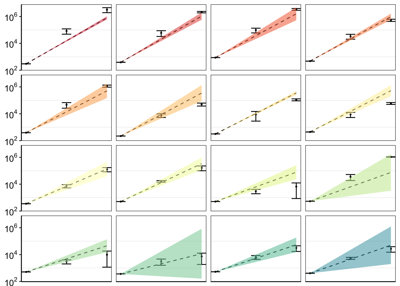

ggsave("pooled_growth_fig_cifrom4paramlogistic_060420.pdf",width=3,height=3,units="in",useDingbats=F)

1. Figure out why your less resistant mutants appear to be more resistant than the IC50 predictions in these plots. Especially because I don’t see that in the observed vs expected plots. Answer: IC50 values tend to underestimate the growth rate of the more sensitive variants. When I fix this with a 4-parameter logistic fit, it looks much better.

2. For Shendure, instead of plotting on the same plot, plot the fold change values over time. Where are you getting the predictions from? Would it be possible to make the predictions based off of the MAFs?

Next step: Is our method better than the Shendure method? 1. Can they make accurate predicitons? Can you use just mutant allele frequency, without count data? I.e. does that data match expected growth? 2. Does their method still work for measuring gain of funciton phenotypes? 3. Do they have enough coverage given a detection efficiency of 10,000? Assume you make 1,000 mutants Given a detection efficiency of 1 in 10,000, for mutants treated with drug for a specified amount of time, how many mutants will you get enough coverage for?

Session information

sessionInfo()

R version 4.0.0 (2020-04-24)
Platform: x86_64-apple-darwin17.0 (64-bit)
Running under: macOS Catalina 10.15.4

Matrix products: default
BLAS:   /Library/Frameworks/R.framework/Versions/4.0/Resources/lib/libRblas.dylib
LAPACK: /Library/Frameworks/R.framework/Versions/4.0/Resources/lib/libRlapack.dylib

locale:
[1] en_US.UTF-8/en_US.UTF-8/en_US.UTF-8/C/en_US.UTF-8/en_US.UTF-8

attached base packages:
[1] parallel  grid      stats     graphics  grDevices utils     datasets 
[8] methods   base     

other attached packages:
 [1] drc_3.0-1           MASS_7.3-51.5       BiocManager_1.30.10
 [4] plotly_4.9.2.1      ggsignif_0.6.0      devtools_2.3.0     
 [7] usethis_1.6.1       RColorBrewer_1.1-2  reshape2_1.4.4     
[10] ggplot2_3.3.0       doParallel_1.0.15   iterators_1.0.12   
[13] foreach_1.5.0       dplyr_0.8.5         VennDiagram_1.6.20 
[16] futile.logger_1.4.3 tictoc_1.0          knitr_1.28         
[19] workflowr_1.6.2    

loaded via a namespace (and not attached):
 [1] fs_1.4.1             httr_1.4.1           rprojroot_1.3-2     
 [4] tools_4.0.0          backports_1.1.7      R6_2.4.1            
 [7] lazyeval_0.2.2       colorspace_1.4-1     withr_2.2.0         
[10] tidyselect_1.1.0     prettyunits_1.1.1    processx_3.4.2      
[13] curl_4.3             compiler_4.0.0       git2r_0.27.1        
[16] cli_2.0.2            formatR_1.7          sandwich_2.5-1      
[19] desc_1.2.0           labeling_0.3         scales_1.1.1        
[22] mvtnorm_1.1-0        callr_3.4.3          stringr_1.4.0       
[25] digest_0.6.25        foreign_0.8-78       rmarkdown_2.1       
[28] rio_0.5.16           pkgconfig_2.0.3      htmltools_0.4.0     
[31] sessioninfo_1.1.1    plotrix_3.7-8        htmlwidgets_1.5.1   
[34] rlang_0.4.6          readxl_1.3.1         farver_2.0.3        
[37] zoo_1.8-8            jsonlite_1.6.1       crosstalk_1.1.0.1   
[40] gtools_3.8.2         zip_2.0.4            car_3.0-7           
[43] magrittr_1.5         Matrix_1.2-18        Rcpp_1.0.4.6        
[46] munsell_0.5.0        fansi_0.4.1          abind_1.4-5         
[49] lifecycle_0.2.0      stringi_1.4.6        multcomp_1.4-13     
[52] whisker_0.4          yaml_2.2.1           carData_3.0-3       
[55] pkgbuild_1.0.8       plyr_1.8.6           promises_1.1.0      
[58] forcats_0.5.0        crayon_1.3.4         lattice_0.20-41     
[61] splines_4.0.0        haven_2.2.0          hms_0.5.3           
[64] ps_1.3.3             pillar_1.4.4         codetools_0.2-16    
[67] pkgload_1.0.2        futile.options_1.0.1 glue_1.4.1          
[70] evaluate_0.14        lambda.r_1.2.4       data.table_1.12.8   
[73] remotes_2.1.1        vctrs_0.3.0          httpuv_1.5.2        
[76] testthat_2.3.2       cellranger_1.1.0     gtable_0.3.0        
[79] purrr_0.3.4          tidyr_1.0.3          assertthat_0.2.1    
[82] xfun_0.13            openxlsx_4.1.5       later_1.0.0         
[85] survival_3.1-12      viridisLite_0.3.0    tibble_3.0.1        
[88] memoise_1.1.0        TH.data_1.0-10       ellipsis_0.3.1