enrichment_simulations

Last updated: 2020-08-13

Checks: 6 1

Knit directory: duplex_sequencing_screen/

This reproducible R Markdown analysis was created with workflowr (version 1.6.2). The Checks tab describes the reproducibility checks that were applied when the results were created. The Past versions tab lists the development history.

R Markdown file: uncommitted changes

The R Markdown file has unstaged changes. To know which version of the R Markdown file created these results, you’ll want to first commit it to the Git repo. If you’re still working on the analysis, you can ignore this warning. When you’re finished, you can run wflow_publish to commit the R Markdown file and build the HTML.

Environment: empty

Great job! The global environment was empty. Objects defined in the global environment can affect the analysis in your R Markdown file in unknown ways. For reproduciblity it’s best to always run the code in an empty environment.

Seed: set.seed(20200402)

The command set.seed(20200402) was run prior to running the code in the R Markdown file. Setting a seed ensures that any results that rely on randomness, e.g. subsampling or permutations, are reproducible.

Session information: recorded

Great job! Recording the operating system, R version, and package versions is critical for reproducibility.

Cache: none

Nice! There were no cached chunks for this analysis, so you can be confident that you successfully produced the results during this run.

File paths: relative

Great job! Using relative paths to the files within your workflowr project makes it easier to run your code on other machines.

Repository version: c0b2ec0

Great! You are using Git for version control. Tracking code development and connecting the code version to the results is critical for reproducibility.

The results in this page were generated with repository version c0b2ec0. See the Past versions tab to see a history of the changes made to the R Markdown and HTML files.

Note that you need to be careful to ensure that all relevant files for the analysis have been committed to Git prior to generating the results (you can use wflow_publish or wflow_git_commit). workflowr only checks the R Markdown file, but you know if there are other scripts or data files that it depends on. Below is the status of the Git repository when the results were generated:


Ignored files:
    Ignored:    .Rhistory
    Ignored:    .Rproj.user/

Untracked files:
    Untracked:  10kmutants_nowt.csv
    Untracked:  10kmutants_wt_1_1.csv
    Untracked:  Rplot.png
    Untracked:  Rplot01.pdf
    Untracked:  allele_freq_enrichment_sim.pdf
    Untracked:  allmuts_dose_response.pdf
    Untracked:  analysis/bcrabl_hill_ic50s.csv
    Untracked:  analysis/column_definitions_for_twinstrand_data_06062020.csv
    Untracked:  analysis/dose_response_curve_fitting_with_errorbars.Rmd
    Untracked:  analysis/multinomial_sims.Rmd
    Untracked:  analysis/mutagenesis_radar_chart.Rmd
    Untracked:  analysis/simple_data_generation.Rmd
    Untracked:  analysis/twinstrand_growthrates_simple.csv
    Untracked:  analysis/twinstrand_maf_merge_simple.csv
    Untracked:  analysis/wildtype_growthrates_sequenced.csv
    Untracked:  bcrablwt_dose_response.pdf
    Untracked:  code/microvariation.normalizer.R
    Untracked:  count_enrichment_sim.pdf
    Untracked:  data/Combined_data_frame_IC_Mutprob_abundance.csv
    Untracked:  data/IC50HeatMap.csv
    Untracked:  data/Twinstrand/
    Untracked:  data/gfpenrichmentdata.csv
    Untracked:  data/heatmap_concat_data.csv
    Untracked:  data/mcmc_inferred_doses.csv
    Untracked:  dosing_error_doseresponse.pdf
    Untracked:  dosing_error_doseresponse_forgrant.pdf
    Untracked:  e255k_dose_response.pdf
    Untracked:  e255k_initial_spikins_figure.pdf
    Untracked:  enrichment_simulations_3mutant_MAF.pdf
    Untracked:  enrichment_simulations_3mutant_count.pdf
    Untracked:  figures_archive/
    Untracked:  inferred_doses_barplot_werrorbars.pdf
    Untracked:  inferred_doses_barplot_werrorbars_wt.pdf
    Untracked:  inferred_doses_caterpillar.pdf
    Untracked:  inferred_doses_caterpillar2.pdf
    Untracked:  inferred_doses_violin.pdf
    Untracked:  output/archive/
    Untracked:  output/bmes_abstract_51220.pdf
    Untracked:  output/clinicalabundancepredictions_BMES_abstract_51320.pdf
    Untracked:  output/clinicalabundancepredictions_BMES_abstract_52020.pdf
    Untracked:  output/enrichment_simulations_3mutants_52020.pdf
    Untracked:  output/grant_fig.pdf
    Untracked:  output/grant_fig_v2.pdf
    Untracked:  output/grant_fig_v2updated.pdf
    Untracked:  output/ic50data_all_conc.csv
    Untracked:  output/ic50data_all_confidence_intervals_individual_logistic_fits.csv
    Untracked:  output/ic50data_all_confidence_intervals_raw_data.csv
    Untracked:  output/ic50heatmap_sd_ci.csv
    Untracked:  output/twinstrand_microvariations_normalized.csv
    Untracked:  shinyapp/

Unstaged changes:
    Modified:   analysis/4_7_20_update.Rmd
    Modified:   analysis/E255K_alphas_figure.Rmd
    Modified:   analysis/clinical_abundance_predictions.Rmd
    Modified:   analysis/dose_response_curve_fitting.Rmd
    Modified:   analysis/enrichment_simulations.Rmd
    Modified:   analysis/misc.Rmd
    Modified:   analysis/nonlinear_growth_analysis.Rmd
    Modified:   analysis/spikeins_depthofcoverages.Rmd
    Modified:   analysis/twinstrand_spikeins_data_generation.Rmd
    Deleted:    data/README.md
    Modified:   output/twinstrand_maf_merge.csv
    Modified:   output/twinstrand_simple_melt_merge.csv

Note that any generated files, e.g. HTML, png, CSS, etc., are not included in this status report because it is ok for generated content to have uncommitted changes.

These are the previous versions of the repository in which changes were made to the R Markdown (analysis/enrichment_simulations.Rmd) and HTML (docs/enrichment_simulations.html) files. If you’ve configured a remote Git repository (see ?wflow_git_remote), click on the hyperlinks in the table below to view the files as they were in that past version.

File	Version	Author	Date	Message
html	d5c685e	haiderinam	2020-06-02	Build site.
Rmd	9af89d9	haiderinam	2020-06-02	wflow_publish(“analysis/enrichment_simulations.Rmd”)

# rm(list=ls())
library(knitr)
library(tictoc)
library(workflowr)

This is workflowr version 1.6.2
Run ?workflowr for help getting started

library(VennDiagram)

Loading required package: grid

Loading required package: futile.logger

library(dplyr)


Attaching package: 'dplyr'

The following objects are masked from 'package:stats':

    filter, lag

The following objects are masked from 'package:base':

    intersect, setdiff, setequal, union

library(foreach)
library(doParallel)

Loading required package: iterators

Loading required package: parallel

library(ggplot2)
library(reshape2)
library(RColorBrewer)
library(devtools)

Loading required package: usethis

library(ggsignif)
library(plotly)


Attaching package: 'plotly'

The following object is masked from 'package:ggplot2':

    last_plot

The following object is masked from 'package:stats':

    filter

The following object is masked from 'package:graphics':

    layout

library(BiocManager)

Bioconductor version 3.11 (BiocManager 1.30.10), ?BiocManager::install for help


Attaching package: 'BiocManager'

The following object is masked from 'package:devtools':

    install

library(drc)

Loading required package: MASS


Attaching package: 'MASS'

The following object is masked from 'package:plotly':

    select

The following object is masked from 'package:dplyr':

    select


'drc' has been loaded.

Please cite R and 'drc' if used for a publication,

for references type 'citation()' and 'citation('drc')'.


Attaching package: 'drc'

The following objects are masked from 'package:stats':

    gaussian, getInitial

library("lmtest")

Loading required package: zoo


Attaching package: 'zoo'

The following objects are masked from 'package:base':

    as.Date, as.Date.numeric

library("ggplot2")
library("MASS")
library("fitdistrplus")

Loading required package: survival

Loading required package: npsurv

Loading required package: lsei

library("lme4")

Loading required package: Matrix

Registered S3 methods overwritten by 'lme4':
  method                          from
  cooks.distance.influence.merMod car 
  influence.merMod                car 
  dfbeta.influence.merMod         car 
  dfbetas.influence.merMod        car

library("boot")


Attaching package: 'boot'

The following object is masked from 'package:survival':

    aml

library("dplyr")
library("plotly")
library(drc)
library(devtools)
library(deSolve)
library(RColorBrewer)
library(reshape2)
######################Cleanup for GGPlot2#########################################



net_gr_wodrug=1.4
# ic50data_long=read.csv("../output/ic50data_all_conc.csv",header = T,stringsAsFactors = F)
ic50data_long=read.csv("output/ic50data_all_conc.csv",header = T,stringsAsFactors = F)
ic50data_long$netgr_pred=net_gr_wodrug-ic50data_long$drug_effect


# twinstrand_simple_melt_merge=read.csv("../output/twinstrand_simple_melt_merge.csv",header = T,stringsAsFactors = F)
twinstrand_simple_melt_merge=read.csv("output/twinstrand_simple_melt_merge.csv",header = T,stringsAsFactors = F)

cleanup=theme_bw() +
  theme(plot.title = element_text(hjust=.5),
        panel.grid.major = element_blank(),
        panel.grid.major.y = element_blank(),
        panel.background = element_blank(),
        # axis.line = element_line(color = "black"),
        axis.text = element_text(face="bold",color="black",size="11"),
        text=element_text(size=11,face="bold"),
        axis.title=element_text(face="bold",size="11"))

1:1000 mixture in a total of 20M cells

ic50data_long=ic50data_long%>%filter(conc%in%c(.3,.6,1.2,2.4))
#In the next step, I'm ordering mutants by decreasing resposne to the 625nM dose. Then I use this to change the levels of the species factor from more to less resistant. This helps with ggplot because now I can color the mutants with decreasing resistance
ic50data_long_625=ic50data_long%>%filter(conc==.6)
ic50data_long$mutant=factor(ic50data_long$mutant,levels = as.character(ic50data_long_625$mutant[order((ic50data_long_625$y),decreasing = T)]))

# ic50data_long$mutant=factor(ic50data_long$mutant,levels = as.character(ic50data_long_625$mutant[order((ic50data_long_625$y),decreasing = T)]))

# rm(list=ls())
# growthrate_nodrug=1.1 ##1.1 means a 15 hour doubling time
growthrate_nodrug=1.4 ##1.4 means a 12 hour doubling time
t=0:6


# ic50data_long$mutant=factor(ic50data_long$mutant,ordered = T)
# ic50data=dcast(data = ic50data_long,conc~mutant)
#Ideally, we would fit a 4 parameter logistic to this and then get the predicted 625 values
# x0=c(15000000,15000,15000,15000,15000,15000,15000,15000,15000,15000,15000,15000,15000,15000,15000,15000,15000,15000,15000,39*15000,56*15000,15000)
# trying out 1:10,000
x0=c(15000,15000/2.5,15000,15000,15000,15000,15000,15000,15000,15000,15000,15000,15000,15000,15000,15000,15000,39*15000,15000,100*15000,15000,56*15000)
sum(x0)

[1] 3201000

sol_comb_doses=data.frame()
# for(j in 1:length(ic50data[,1])){
for(dose in sort(unique(ic50data_long$conc))){
  # dose=.8
  #Grabbing net growth rate at desired concentration
  ic50data_specificdose=ic50data_long%>%filter(conc==dose)
  # ic50data_specificdose$mutant
  ic50data_specificdose$drugeffect=-log(ic50data_specificdose$y_model)/3
  ic50data_specificdose$growthrate_net=growthrate_nodrug-ic50data_specificdose$drugeffect
  
##Differential equation function
cgrowth=function(times,y,params){
  dN.dt=ic50data_specificdose$growthrate_net[i]*y[1]
  return(list(dN.dt))
}
sol_comb=data.frame()
for(i in 1:length(ic50data_specificdose[,1])){
sol=ode(y=x0[i],times=t,func=cgrowth,parms=growthrate_net[i])
sol_df=data.frame(sol)
sol_df$mutant=ic50data_specificdose$mutant[i]
# ic50data_specificdose$mutant[2]
  # colnames(growthrate_net[i])
sol_comb=rbind(sol_comb,data.frame(sol_df))
}
colnames(sol_comb)[colnames(sol_comb)=="X1"]="count"
# sol_comb$dose=ic50data$conc[j]
sol_comb$dose=dose
sol_comb_doses=rbind(sol_comb_doses,sol_comb)
}

#Plotting total # of cells
getPalette = colorRampPalette(brewer.pal(9, "Spectral"))

#Wt grows unless the drug concentration is like 625nM
# ggplot(data=sol_comb_doses,aes(y=count,x=time,color=factor(mutant)))+geom_line()+facet_wrap(~dose)+cleanup+scale_color_manual(values = getPalette(length(unique(sol_comb_doses$mutant))))
# 
# ggplot(data=sol_comb_doses,aes(time,count))+
#   geom_col(aes(fill=mutant))+
#   facet_wrap(~dose)+
#   cleanup+
#   scale_fill_manual(values = getPalette(length(unique(sol_comb_doses$mutant))))
# 
# #Log scale shows that other mutants are actually growing too
# ggplot(data=sol_comb_doses,aes(y=log(count),x=time,color=factor(mutant)))+geom_line()+facet_wrap(~dose)+cleanup+scale_color_manual(values = getPalette(length(unique(sol_comb_doses$mutant))))


sol_comb_doses=sol_comb_doses%>%group_by(dose,time)%>%mutate(total=sum(count))%>%group_by(dose,time,mutant)%>%mutate(proportion=count/total)

###Looking at the proportion of mutants given various starting doses
ggplot(data=sol_comb_doses,aes(time,proportion))+geom_col(aes(fill=mutant))+geom_line(aes(y=total/max(sol_comb_doses$total)))+scale_y_continuous(sec.axis = sec_axis(~.*max(sol_comb_doses$total), name = "Total Count"))+facet_wrap(~dose)+cleanup+scale_fill_manual(values = getPalette(length(unique(sol_comb_doses$mutant))))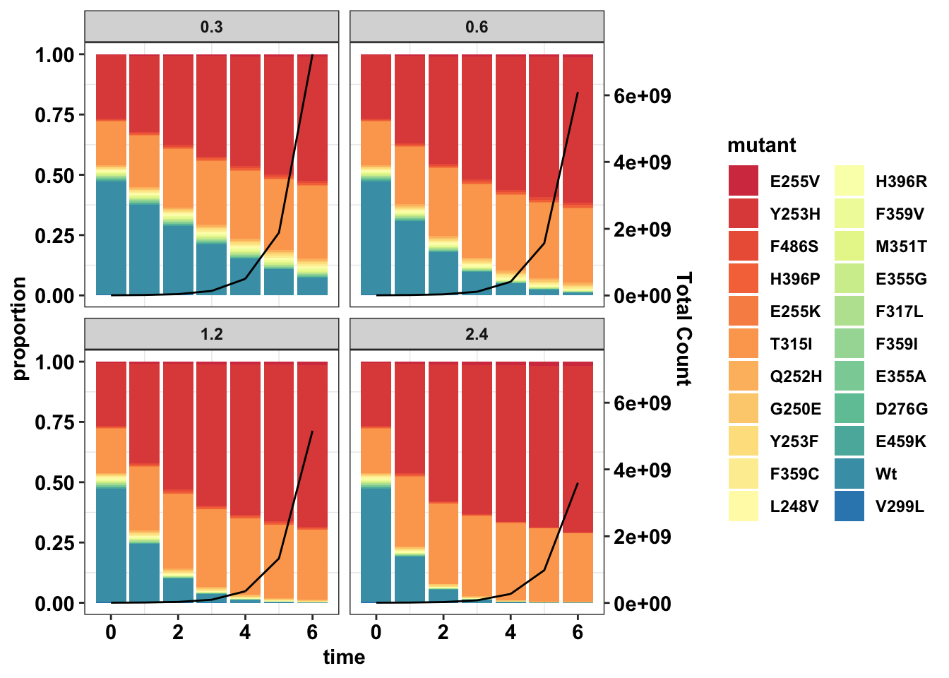

Version	Author	Date
d5c685e	haiderinam	2020-06-02

##Looking closely at just one plot
  x=ggplot(data=sol_comb_doses%>%filter(dose==0.6),aes(time,proportion))+
    geom_col(aes(fill=mutant))+
    geom_line(aes(y=total/max(sol_comb_doses$total)))+
    scale_y_continuous(sec.axis = sec_axis(~.*max(sol_comb_doses$total), name = "Total Count"))+facet_wrap(~dose)+
    cleanup+
    scale_fill_manual(values = getPalette(length(unique(sol_comb_doses$mutant))))
  ggplotly(x)

  #Can also use this for coloring (doesn't require counting the 22 mutants)
  # palette_Dark2 <- colorRampPalette(brewer.pal(14, "Set2"))
  # +discrete_scale("fill", "manual", palette_Dark2)

# a=sol_comb_doses%>%filter(!mutant%in%c("F359Lmini","M244V","F359Lmaxi","V299L_L","V299L_H","V299L_H","D276G"))%>%group_by(dose,time)%>%summarize(min_coverage=100/min(proportion),min_coverage_sp=mutant[proportion==min(proportion)][1])
#Check that D275G is resistant
a=sol_comb_doses%>%filter(time%in%c(0,3,6),dose==.6)
# write.csv(sol_comb_doses,"10kmutants_wt_1_1.csv")
b=ic50data_specificdose$mutant
aa=sol_comb_doses%>%filter(mutant%in%"E255K")%>%mutate(percent=proportion*100)
aa=sol_comb_doses%>%filter(time%in%4)%>%mutate(percent=proportion*100)

e255kdiagnostics=twinstrand_simple_melt_merge%>%filter(mutant%in%"E255K",experiment%in%"M6")
e255kdiagnostics=twinstrand_simple_melt_merge%>%filter(mutant%in%"E255K",experiment%in%"M5")

# ic50data_long2=ic50data_long
ic50data_long=ic50data_long%>%filter(mutant%in%c("T315I","L248V","E355A"))
# rm(list=ls())
# growthrate_nodrug=1.1 ##1.1 means a 15 hour doubling time
growthrate_nodrug=1.4 ##1.4 means a 12 hour doubling time
t=0:8


# ic50data_long$mutant=factor(ic50data_long$mutant,ordered = T)
# ic50data=dcast(data = ic50data_long,conc~mutant)
#Ideally, we would fit a 4 parameter logistic to this and then get the predicted 625 values
# x0=c(15000000,15000,15000,15000,15000,15000,15000,15000,15000,15000,15000,15000,15000,15000,15000,15000,15000,15000,15000,39*15000,56*15000,15000)
# trying out 1:10,000
x0=c(10000000,10000000,10000000)

sol_comb_doses=data.frame()
# for(j in 1:length(ic50data[,1])){
for(dose in sort(unique(ic50data_long$conc))){
  # dose=.8
  #Grabbing net growth rate at desired concentration
  ic50data_specificdose=ic50data_long%>%filter(conc==dose)
  ic50data_specificdose$drugeffect=-log(ic50data_specificdose$y_model)/3
  ic50data_specificdose$growthrate_net=growthrate_nodrug-ic50data_specificdose$drugeffect
  
##Differential equation function
cgrowth=function(times,y,params){
  dN.dt=ic50data_specificdose$growthrate_net[i]*y[1]
  return(list(dN.dt))
}
sol_comb=data.frame()
for(i in 1:length(ic50data_specificdose[,1])){
sol=ode(y=x0[i],times=t,func=cgrowth,parms=growthrate_net[i])
sol_df=data.frame(sol)
sol_df$mutant=ic50data_specificdose$mutant[i]
  # colnames(growthrate_net[i])
sol_comb=rbind(sol_comb,data.frame(sol_df))
}
colnames(sol_comb)[colnames(sol_comb)=="X1"]="count"
# sol_comb$dose=ic50data$conc[j]
sol_comb$dose=dose
sol_comb_doses=rbind(sol_comb_doses,sol_comb)
}

#Plotting total # of cells
getPalette = colorRampPalette(brewer.pal(9, "Spectral"))

ggplot(data=sol_comb_doses,aes(time,count))+
  geom_col(aes(fill=mutant))+
  facet_wrap(~dose)+
  cleanup+
  scale_fill_manual(values = getPalette(length(unique(sol_comb_doses$mutant))))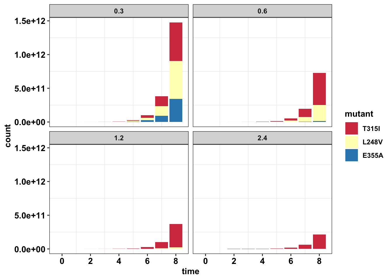

Version	Author	Date
d5c685e	haiderinam	2020-06-02

#Log scale shows that other mutants are actually growing too
ggplot(data=sol_comb_doses,aes(y=log(count),x=time,color=factor(mutant)))+geom_line()+facet_wrap(~dose)+cleanup+scale_color_manual(values = getPalette(length(unique(sol_comb_doses$mutant))))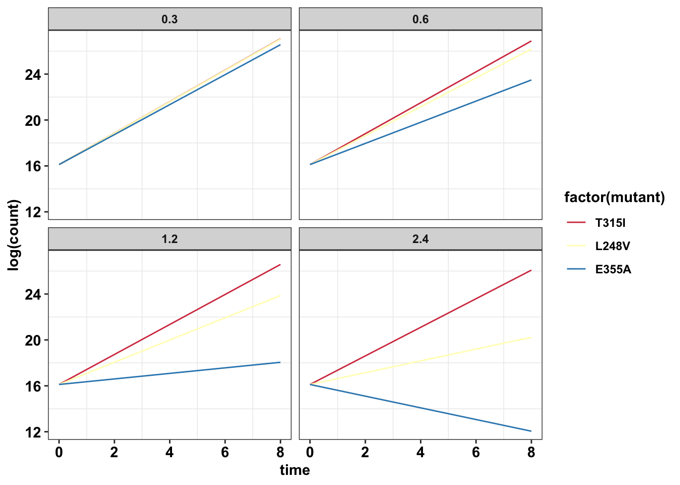

Version	Author	Date
d5c685e	haiderinam	2020-06-02

sol_comb_doses=sol_comb_doses%>%group_by(dose,time)%>%mutate(total=sum(count))%>%group_by(dose,time,mutant)%>%mutate(proportion=count/total)

###Looking at the proportion of mutants given various starting doses
ggplot(data=sol_comb_doses,aes(time,proportion))+geom_col(aes(fill=mutant))+geom_line(aes(y=total/max(sol_comb_doses$total)))+scale_y_continuous(sec.axis = sec_axis(~.*max(sol_comb_doses$total), name = "Total Count"))+facet_wrap(~dose)+cleanup+scale_fill_manual(values = getPalette(length(unique(sol_comb_doses$mutant))))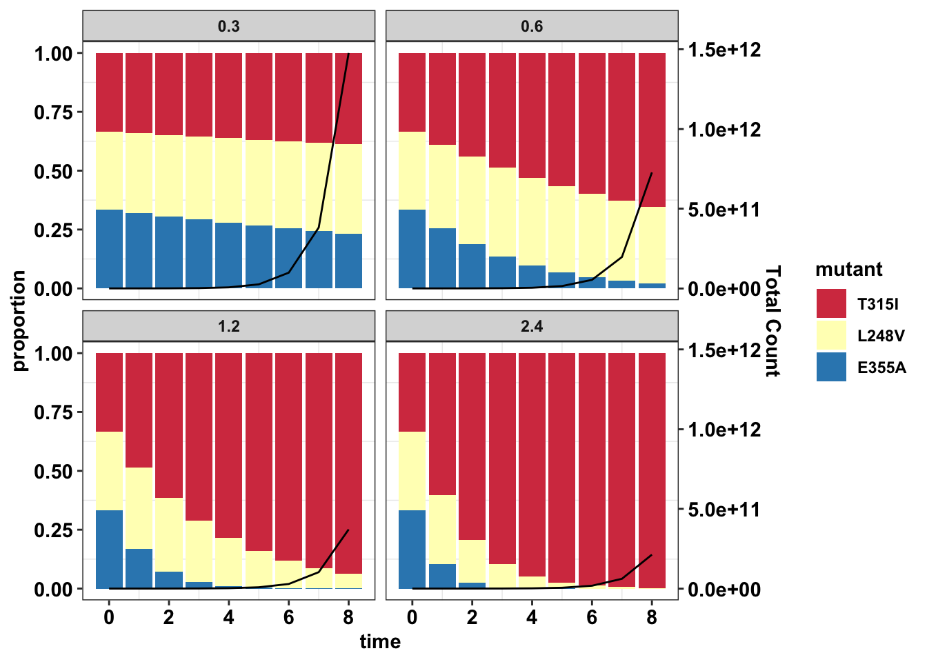

Version	Author	Date
d5c685e	haiderinam	2020-06-02

#Can also use this for coloring (doesn't require counting the 22 mutants)
  palette_Dark2 <- colorRampPalette(brewer.pal(14, "Set2"))

Warning in brewer.pal(14, "Set2"): n too large, allowed maximum for palette Set2 is 8
Returning the palette you asked for with that many colors

  # +discrete_scale("fill", "manual", palette_Dark2)
  
##Looking closely at just one plot
  sol_comb_doses$mutant=factor(sol_comb_doses$mutant,levels=c("E355A","L248V","T315I"))
  x=ggplot(data=sol_comb_doses%>%filter(dose==1.2),aes(time,proportion))+
    geom_col(aes(fill=mutant))+
    # geom_line(aes(y=total/max(sol_comb_doses$total)))+
    # scale_y_continuous(sec.axis = sec_axis(~.*max(sol_comb_doses$total), name = "Total Count"))+
    # facet_wrap(~dose)+
    cleanup+
    discrete_scale("fill", "manual", palette_Dark2)+
    scale_x_continuous(expand = c(0,0),name = "Time (Days)")+
    scale_y_continuous(expand = c(0,0),name = "Mutant Allele Fraction")+
    theme(panel.grid.major = element_blank(),
            panel.grid.minor = element_blank(),
            panel.background = element_blank(),
            axis.line = element_line(colour = "black"))
    # theme(plot.title = element_text(hjust=.5),text = element_text(size=30,face="bold"),axis.title = element_text(face="bold",size="26"),axis.text=element_text(face="bold",color="black",size="26"))
    # scale_fill_manual(values = getPalette(length(unique(sol_comb_doses$mutant))))
ggplotly(x)

# ggsave("enrichment_simulations_3mutants.pdf",width = 4,height = 3,units = "in",useDingbats=F)  

########Analysis trying to show that there is a real depletion effecf:
ggplot(sol_comb_doses%>%filter(time<=6,dose%in%1.2),aes(x=time,y=proportion,group=mutant))+
  geom_line()+
  geom_point(color="black",shape=21,size=2,aes(fill=factor(mutant)))+
  cleanup+
  discrete_scale("fill", "manual", palette_Dark2)+
  discrete_scale("color", "manual", palette_Dark2)+
  scale_y_continuous(name="Mutant Allele Fraction")+
  scale_x_continuous(name="Time (Days)")+
  theme(legend.position = "none",
        axis.title = element_text(face="bold",size=10),
        axis.text = element_text(face="plain",size=9))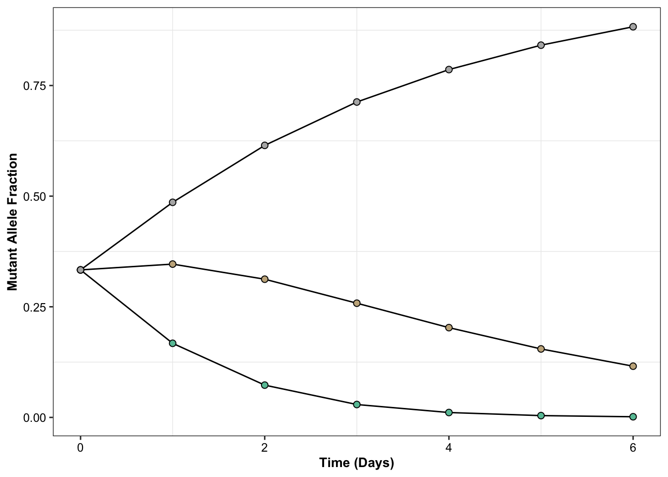

# ggsave("enrichment_simulations_3mutant_MAF.pdf",width=2,height=2,units="in",useDingbats=F)

ggplot(sol_comb_doses%>%filter(time<=6,dose%in%1.2),aes(x=time,y=count,group=mutant))+
  geom_line()+
  geom_point(color="black",shape=21,size=2,aes(fill=factor(mutant)))+
  cleanup+
  discrete_scale("fill", "manual", palette_Dark2)+
  discrete_scale("color", "manual", palette_Dark2)+
  scale_y_continuous(name="Mutant Count",trans="log10",breaks=c(1e7,1e8,1e9,1e10),labels=parse(text=c("10^7","10^8","10^9","10^10")))+
  # scale_y_continuous(name="Mutant Count",breaks=c(0,1e10,2e10),labels=parse(text=c("0","10^10","2*10^10")))+
  scale_x_continuous(name="Time (Days)")+
  theme(legend.position = "none",
        axis.title = element_text(face="bold",size=10),
        axis.text = element_text(face="plain",size=9))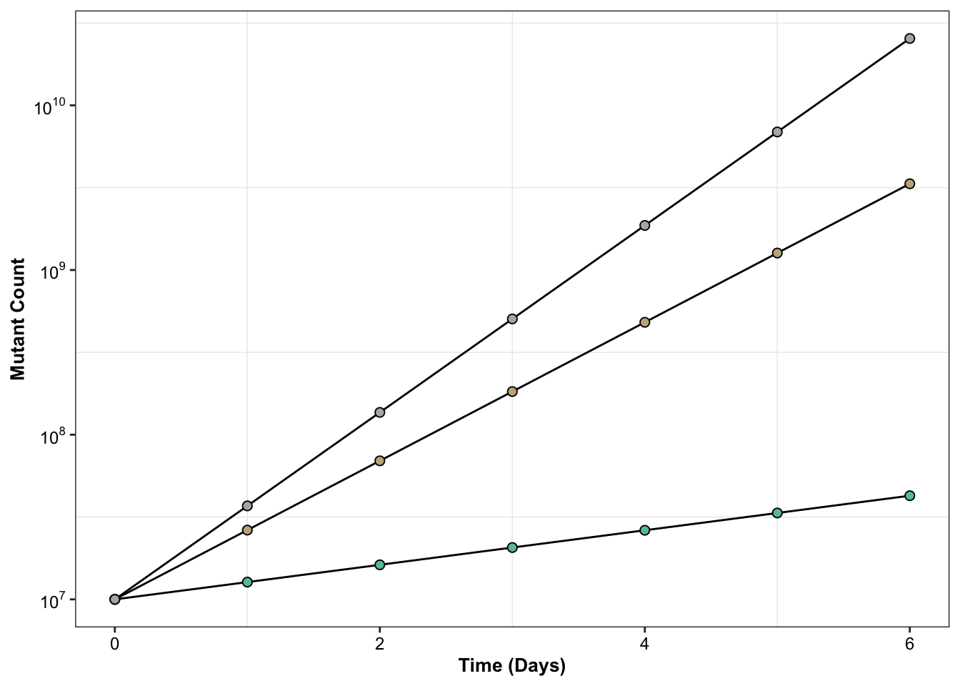

# ggsave("enrichment_simulations_3mutant_count.pdf",width=2,height=2,units="in",useDingbats=F)

ggplot(sol_comb_doses%>%filter(dose%in%1.2)%>%filter(time%in%c(0,3)),aes(x=(factor(time)),y=proportion,fill=factor(mutant)))+geom_col(color="black")+facet_wrap(~mutant)+cleanup+discrete_scale("fill", "manual", palette_Dark2)+
  scale_y_continuous(name="Mutant Allele Fraction",expand = c(0.01,0))+
  scale_x_discrete(name="Time (Days)")+
  theme(strip.text = element_blank(),
        legend.position = "none",
        axis.title = element_text(face="bold",size=10),
        axis.text = element_text(face="plain",size=9))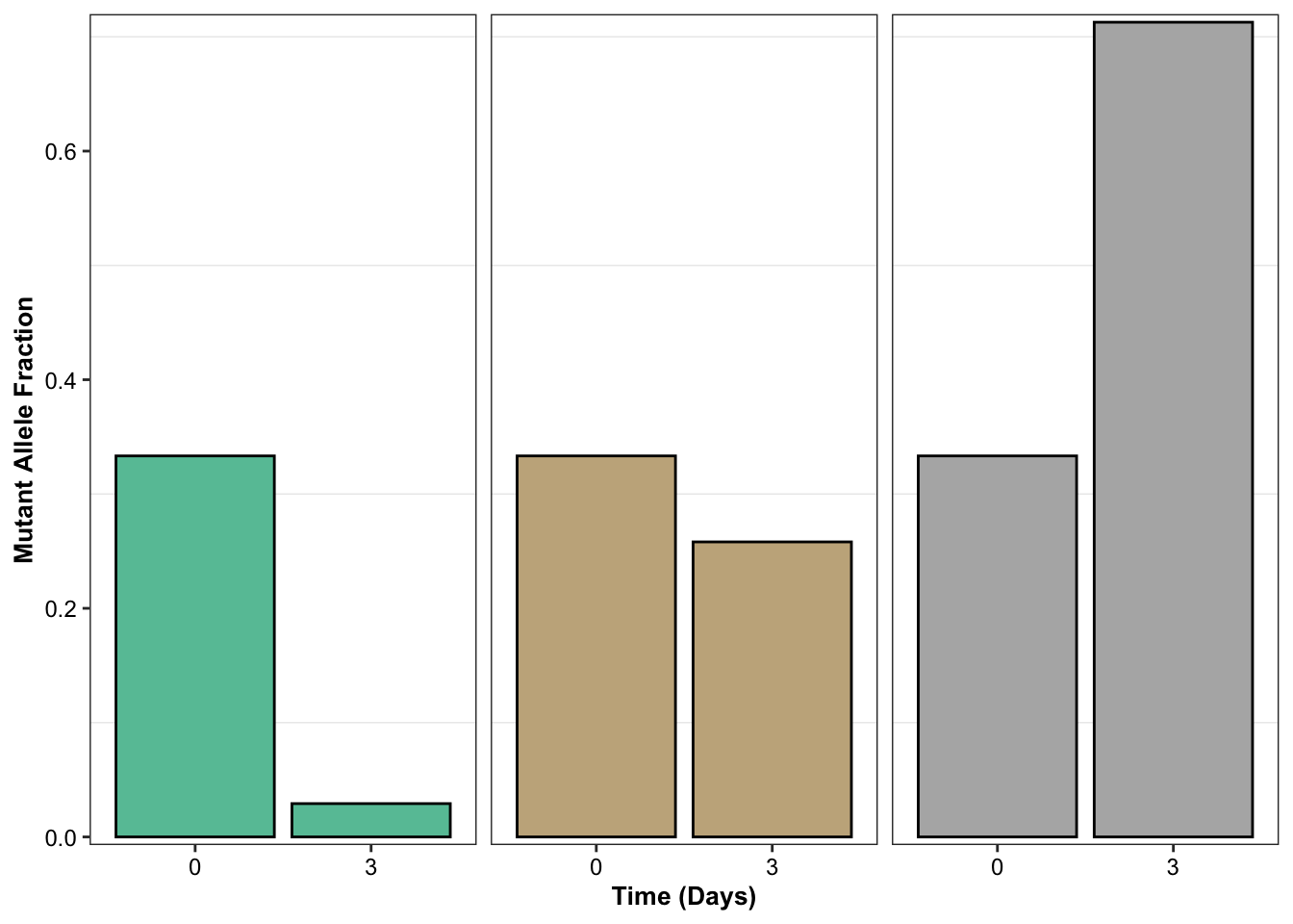

# ggsave("allele_freq_enrichment_sim.pdf",width=3,height=2,units="in",useDingbats=F)

ggplot(sol_comb_doses%>%filter(dose%in%1.2)%>%filter(time%in%c(0,3)),aes(x=(factor(time)),y=count,fill=factor(mutant)))+geom_col(color="black")+facet_wrap(~mutant)+cleanup+discrete_scale("fill", "manual", palette_Dark2)+
  scale_y_continuous(name="Estimated Counts",
                     expand = c(0.01,0),
                     trans="log10",
                     # limits=c(10^5,10^11),
                     breaks=c(1e6,1e7,1e8,1e9,1e10),
                     labels=parse(text=c("10^6","10^7","10^8","10^9","10^10")))+
  scale_x_discrete(name="Time (Days)")+
  theme(strip.text = element_blank(),
        legend.position = "none",
        axis.title = element_text(face="bold",size=10),
        axis.text = element_text(face="plain",size=9))+
  coord_cartesian(ylim = c(10^6, 10^9))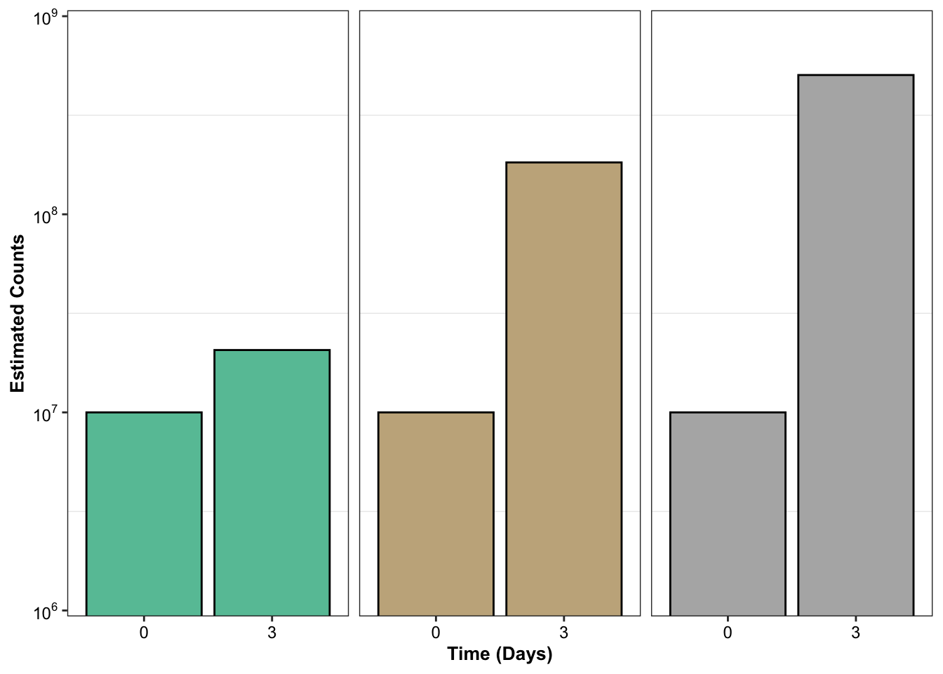

# ggsave("count_enrichment_sim.pdf",width=3,height=2,units="in",useDingbats=F)

sessionInfo()

R version 4.0.0 (2020-04-24)
Platform: x86_64-apple-darwin17.0 (64-bit)
Running under: macOS Catalina 10.15.6

Matrix products: default
BLAS:   /Library/Frameworks/R.framework/Versions/4.0/Resources/lib/libRblas.dylib
LAPACK: /Library/Frameworks/R.framework/Versions/4.0/Resources/lib/libRlapack.dylib

locale:
[1] en_US.UTF-8/en_US.UTF-8/en_US.UTF-8/C/en_US.UTF-8/en_US.UTF-8

attached base packages:
[1] parallel  grid      stats     graphics  grDevices utils     datasets 
[8] methods   base     

other attached packages:
 [1] deSolve_1.28        boot_1.3-24         lme4_1.1-23        
 [4] Matrix_1.2-18       fitdistrplus_1.0-14 npsurv_0.4-0.1     
 [7] lsei_1.2-0.1        survival_3.1-12     lmtest_0.9-37      
[10] zoo_1.8-8           drc_3.0-1           MASS_7.3-51.5      
[13] BiocManager_1.30.10 plotly_4.9.2.1      ggsignif_0.6.0     
[16] devtools_2.3.0      usethis_1.6.1       RColorBrewer_1.1-2 
[19] reshape2_1.4.4      ggplot2_3.3.0       doParallel_1.0.15  
[22] iterators_1.0.12    foreach_1.5.0       dplyr_0.8.5        
[25] VennDiagram_1.6.20  futile.logger_1.4.3 workflowr_1.6.2    
[28] tictoc_1.0          knitr_1.28         

loaded via a namespace (and not attached):
 [1] TH.data_1.0-10       minqa_1.2.4          colorspace_1.4-1    
 [4] ellipsis_0.3.1       rio_0.5.16           rprojroot_1.3-2     
 [7] fs_1.4.1             farver_2.0.3         remotes_2.1.1       
[10] fansi_0.4.1          mvtnorm_1.1-0        codetools_0.2-16    
[13] splines_4.0.0        pkgload_1.0.2        jsonlite_1.6.1      
[16] nloptr_1.2.2.1       compiler_4.0.0       httr_1.4.1          
[19] backports_1.1.7      assertthat_0.2.1     lazyeval_0.2.2      
[22] cli_2.0.2            later_1.0.0          formatR_1.7         
[25] htmltools_0.4.0      prettyunits_1.1.1    tools_4.0.0         
[28] gtable_0.3.0         glue_1.4.1           Rcpp_1.0.4.6        
[31] carData_3.0-3        cellranger_1.1.0     vctrs_0.3.0         
[34] nlme_3.1-147         crosstalk_1.1.0.1    xfun_0.13           
[37] stringr_1.4.0        ps_1.3.3             openxlsx_4.1.5      
[40] testthat_2.3.2       lifecycle_0.2.0      gtools_3.8.2        
[43] statmod_1.4.34       scales_1.1.1         hms_0.5.3           
[46] promises_1.1.0       sandwich_2.5-1       lambda.r_1.2.4      
[49] yaml_2.2.1           curl_4.3             memoise_1.1.0       
[52] stringi_1.4.6        desc_1.2.0           plotrix_3.7-8       
[55] pkgbuild_1.0.8       zip_2.0.4            rlang_0.4.6         
[58] pkgconfig_2.0.3      evaluate_0.14        lattice_0.20-41     
[61] purrr_0.3.4          labeling_0.3         htmlwidgets_1.5.1   
[64] processx_3.4.2       tidyselect_1.1.0     plyr_1.8.6          
[67] magrittr_1.5         R6_2.4.1             multcomp_1.4-13     
[70] pillar_1.4.4         haven_2.2.0          whisker_0.4         
[73] foreign_0.8-78       withr_2.2.0          abind_1.4-5         
[76] tibble_3.0.1         crayon_1.3.4         car_3.0-7           
[79] futile.options_1.0.1 rmarkdown_2.1        readxl_1.3.1        
[82] data.table_1.12.8    callr_3.4.3          git2r_0.27.1        
[85] forcats_0.5.0        digest_0.6.25        tidyr_1.0.3         
[88] httpuv_1.5.2         munsell_0.5.0        viridisLite_0.3.0   
[91] sessioninfo_1.1.1

enrichment_simulations

Haider Inam

5/21/2020