Peak Analysis

Last updated: 2025-07-29

Checks: 7 0

Knit directory: WardLab/

This reproducible R Markdown analysis was created with workflowr (version 1.7.1). The Checks tab describes the reproducibility checks that were applied when the results were created. The Past versions tab lists the development history.

R Markdown file: up-to-date

Great! Since the R Markdown file has been committed to the Git repository, you know the exact version of the code that produced these results.

Environment: empty

Great job! The global environment was empty. Objects defined in the global environment can affect the analysis in your R Markdown file in unknown ways. For reproduciblity it’s best to always run the code in an empty environment.

Seed: set.seed(20250701)

The command set.seed(20250701) was run prior to running the code in the R Markdown file. Setting a seed ensures that any results that rely on randomness, e.g. subsampling or permutations, are reproducible.

Session information: recorded

Great job! Recording the operating system, R version, and package versions is critical for reproducibility.

Cache: none

Nice! There were no cached chunks for this analysis, so you can be confident that you successfully produced the results during this run.

File paths: relative

Great job! Using relative paths to the files within your workflowr project makes it easier to run your code on other machines.

Repository version: 63f0b60

Great! You are using Git for version control. Tracking code development and connecting the code version to the results is critical for reproducibility.

The results in this page were generated with repository version 63f0b60. See the Past versions tab to see a history of the changes made to the R Markdown and HTML files.

Note that you need to be careful to ensure that all relevant files for the analysis have been committed to Git prior to generating the results (you can use wflow_publish or wflow_git_commit). workflowr only checks the R Markdown file, but you know if there are other scripts or data files that it depends on. Below is the status of the Git repository when the results were generated:


Ignored files:
    Ignored:    .Rhistory
    Ignored:    .Rproj.user/

Untracked files:
    Untracked:  data/RUVs_DEG.tsv
    Untracked:  data/bam_final/
    Untracked:  data/bam_no_multi/
    Untracked:  data/cutoff_narrow.tsv
    Untracked:  data/cutoff_narrow.tsv.txt
    Untracked:  data/cutoffs.tsv
    Untracked:  data/metadata.txt
    Untracked:  data/multiqc_data_trim/
    Untracked:  data/peaks/
    Untracked:  data/sample_info.tsv
    Untracked:  data/sams/

Unstaged changes:
    Modified:   README.md

Note that any generated files, e.g. HTML, png, CSS, etc., are not included in this status report because it is ok for generated content to have uncommitted changes.

These are the previous versions of the repository in which changes were made to the R Markdown (analysis/peak_analysis.Rmd) and HTML (docs/peak_analysis.html) files. If you’ve configured a remote Git repository (see ?wflow_git_remote), click on the hyperlinks in the table below to view the files as they were in that past version.

File	Version	Author	Date	Message
Rmd	63f0b60	infurnoheat	2025-07-29	wflow_publish("analysis/peak_analysis.Rmd")
html	1160ce2	infurnoheat	2025-07-24	Build site.
Rmd	876d279	infurnoheat	2025-07-24	wflow_publish("analysis/peak_analysis.Rmd")
html	9f8e509	infurnoheat	2025-07-24	Build site.
Rmd	3c31bea	infurnoheat	2025-07-24	wflow_publish("analysis/peak_analysis.Rmd")
html	66c1fa7	infurnoheat	2025-07-24	Build site.
Rmd	5fae1b0	infurnoheat	2025-07-24	wflow_publish("analysis/peak_analysis.Rmd")
html	389b998	infurnoheat	2025-07-23	Build site.
Rmd	1295ae0	infurnoheat	2025-07-23	wflow_publish("analysis/peak_analysis.Rmd")
html	d927f5c	infurnoheat	2025-07-23	Build site.
Rmd	d2f7f9a	infurnoheat	2025-07-23	wflow_publish("analysis/peak_analysis.Rmd")
html	3c5800a	infurnoheat	2025-07-22	Build site.
Rmd	0edadf3	infurnoheat	2025-07-22	wflow_publish("analysis/peak_analysis.Rmd")
html	29d666e	infurnoheat	2025-07-15	Build site.
Rmd	dd8be1d	infurnoheat	2025-07-15	wflow_publish("analysis/peak_analysis.Rmd")
html	1d53459	infurnoheat	2025-07-14	Build site.
Rmd	7067e5d	infurnoheat	2025-07-14	wflow_publish("analysis/peak_analysis.Rmd")

Peak Anaylsis

Loading Packages

library(tidyverse)
library(readr)
library(edgeR)
library(ComplexHeatmap)
library(data.table)
library(dplyr)
library(stringr)
library(ggplot2)
library(viridis)
library(DT)
library(kableExtra)
library(genomation)
library(GenomicRanges)
library(chromVAR) ## For FRiP analysis and differential analysis
library(DESeq2) ## For differential analysis section
library(ggpubr) ## For customizing figures
library(corrplot) ## For correlation plot
library(ggpmisc)
library(gcplyr)
library(Rsubread)

Data Initialization

sampleinfo <- read_delim("data/sample_info.tsv", delim = "\t")
multiqc_gene_stats_trim <- read_delim("data/multiqc_data_trim/multiqc_general_stats.txt",delim = "\t")
multiqc_fastqc_trim <- read_delim("data/multiqc_data_trim/multiqc_fastqc.txt",delim = "\t")

Functions

drug_pal <- c("#8B006D","#DF707E","#F1B72B", "#3386DD","#707031","#41B333")
pca_plot <-
  function(df,
           col_var = NULL,
           shape_var = NULL,
           title = "") {
    ggplot(df) + geom_point(aes_string(
      x = "PC1",
      y = "PC2",
      color = col_var,
      shape = shape_var
    ),
    size = 5) +
      labs(title = title, x = "PC 1", y = "PC 2") +
      scale_color_manual(values = c(
        "#8B006D",
        "#DF707E",
        "#F1B72B",
        "#3386DD",
        "#707031",
        "#41B333"
      ))
  }
pca_var_plot <- function(pca) {
  # x: class == prcomp
  pca.var <- pca$sdev ^ 2
  pca.prop <- pca.var / sum(pca.var)
  var.plot <-
    qplot(PC, prop, data = data.frame(PC = 1:length(pca.prop),
                                      prop = pca.prop)) +
    labs(title = 'Variance contributed by each PC',
         x = 'PC', y = 'Proportion of variance')
  plot(var.plot)
}

calc_pca <- function(x) {
  # Performs principal components analysis with prcomp
  # x: a sample-by-gene numeric matrix
  prcomp(x, scale. = TRUE, retx = TRUE)
}

get_regr_pval <- function(mod) {
  # Returns the p-value for the Fstatistic of a linear model
  # mod: class lm
  stopifnot(class(mod) == "lm")
  fstat <- summary(mod)$fstatistic
  pval <- 1 - pf(fstat[1], fstat[2], fstat[3])
  return(pval)
}

plot_versus_pc <- function(df, pc_num, fac) {
  # df: data.frame
  # pc_num: numeric, specific PC for plotting
  # fac: column name of df for plotting against PC
  pc_char <- paste0("PC", pc_num)
  # Calculate F-statistic p-value for linear model
  pval <- get_regr_pval(lm(df[, pc_char] ~ df[, fac]))
  if (is.numeric(df[, f])) {
    ggplot(df, aes_string(x = f, y = pc_char)) + geom_point() +
      geom_smooth(method = "lm") + labs(title = sprintf("p-val: %.2f", pval))
  } else {
    ggplot(df, aes_string(x = f, y = pc_char)) + geom_boxplot() +
      labs(title = sprintf("p-val: %.2f", pval))
  }
}
x_axis_labels = function(labels, every_nth = 1, ...) {
  axis(side = 1,
       at = seq_along(labels),
       labels = F)
  text(
    x = (seq_along(labels))[seq_len(every_nth) == 1],
    y = par("usr")[3] - 0.075 * (par("usr")[4] - par("usr")[3]),
    labels = labels[seq_len(every_nth) == 1],
    xpd = TRUE,
    ...
  )
}

Peak Calling for Q=0.01 and Broad=0.1 with No Lambda

Data Initialization

peak_ct <- read_delim("data/peaks/peaks_cts.txt", delim = "\t")
H3K27ac_peaks <- read_delim("data/peaks/H3K27ac_final_results.tsv",delim = "\t")
H3K27me3_peaks <- read_delim("data/peaks/H3K27me3_final_results.tsv",delim = "\t")
H3K36me3_peaks <- read_delim("data/peaks/H3K36me3_final_results.tsv",delim = "\t")
H3K9me3_peaks <- read_delim("data/peaks/H3K9me3_final_results.tsv",delim = "\t")

all_peak <- rbind(H3K27ac_peaks, H3K27me3_peaks, H3K36me3_peaks, H3K9me3_peaks)

all_peak <- all_peak %>%
  dplyr::select(Sample, Total_Reads, Fragments, Reads_in_Peaks, FRiP) %>%
  left_join(.,sampleinfo, by=c("Sample"="Library ID")) %>%
  left_join(.,peak_ct, by=c("Sample"="Sample"))
all_peak <- all_peak[(!all_peak$Treatment %in% "5FU"),]

Peak Visualization

all_peak %>% 
   ggplot(.,aes(x=Sample, y=Count,fill=Histone_Mark))+
   geom_col()+
   ylab("Count")+
   theme_classic()+
  # facet_wrap(~histone)+
  ggtitle("Peak number for all samples")+ 
  theme(axis.text.x=element_text(vjust = .2,angle=90))+
  scale_y_continuous( expand = expansion(mult = c(0, .1)))

Version	Author	Date
3c5800a	infurnoheat	2025-07-22
1d53459	infurnoheat	2025-07-14

all_peak %>% 
  ggplot(., aes (x=Histone_Mark, y = Count, fill = Histone_Mark))+
  geom_boxplot()+
   ylab("Count")+
   theme_classic()+
  # facet_wrap(~histone)+
  ggtitle("Peak count across histones")

Version	Author	Date
3c5800a	infurnoheat	2025-07-22
1d53459	infurnoheat	2025-07-14

all_peak %>% 
  ggplot(., aes (x=Treatment, y = Count, fill = Histone_Mark))+
  geom_boxplot()+
   ylab("Count")+
   theme_classic()+
  # facet_wrap(~histone)+
  ggtitle("Peak count across histones")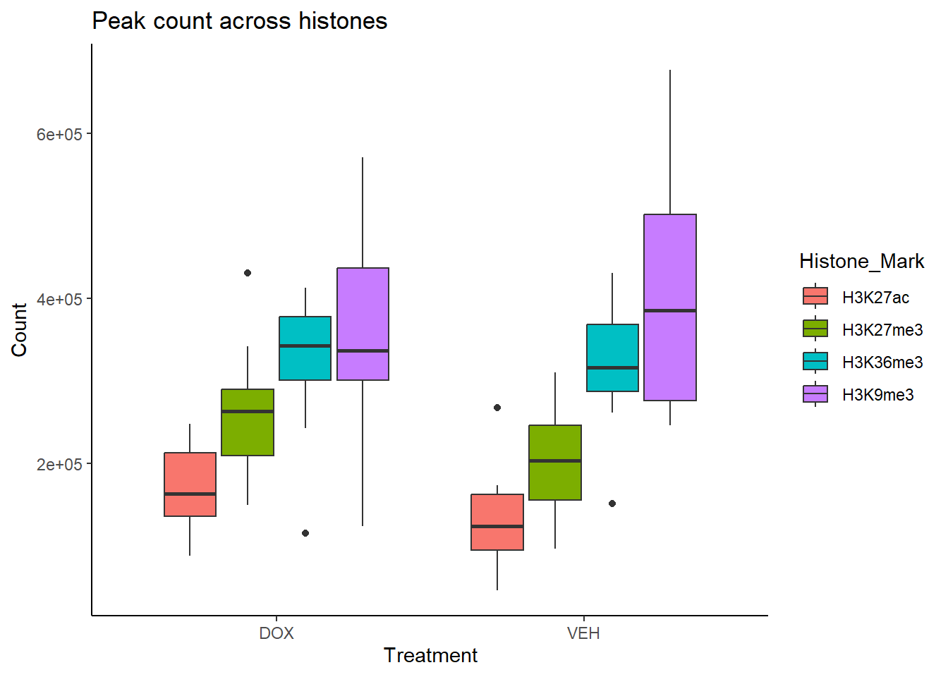

Version	Author	Date
3c5800a	infurnoheat	2025-07-22
1d53459	infurnoheat	2025-07-14

all_peak %>% 
  ggplot(., aes (x=Timepoint, y = Count, fill = Histone_Mark))+
  geom_boxplot()+
   ylab("Count")+
   theme_classic()+
  # facet_wrap(~histone)+
  ggtitle("Peak count across histones")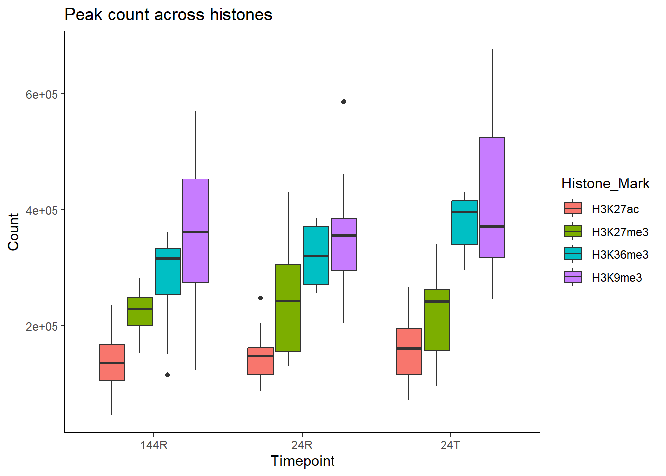

Version	Author	Date
3c5800a	infurnoheat	2025-07-22
1d53459	infurnoheat	2025-07-14

Peak Calling for Q=0.01 and Broad=0.1 with Lambda

Data Initialization

peak_ct <- read_delim("data/peaks/peaks_cts_lq1e2b1e1.txt", delim = "\t")
H3K27ac_peaks <- read_delim("data/peaks/H3K27ac_final_results.tsv",delim = "\t")
H3K27me3_peaks <- read_delim("data/peaks/H3K27me3_lq1e2b1e1_results.tsv",delim = "\t")
H3K36me3_peaks <- read_delim("data/peaks/H3K36me3_lq1e2b1e1_results.tsv",delim = "\t")
H3K9me3_peaks <- read_delim("data/peaks/H3K9me3_lq1e2b1e1_results.tsv",delim = "\t")

all_peak_var <- rbind(H3K27ac_peaks, H3K27me3_peaks, H3K36me3_peaks, H3K9me3_peaks)

all_peak_var <- all_peak_var %>%
  dplyr::select(Sample, Total_Reads, Fragments, Reads_in_Peaks, FRiP) %>%
  left_join(.,sampleinfo, by=c("Sample"="Library ID")) %>%
  left_join(.,peak_ct, by=c("Sample"="Sample"))
all_peak_var <- all_peak_var[(!all_peak_var$Treatment %in% "5FU"),]
all_peak_var <- all_peak_var[(!all_peak_var$Histone_Mark %in% "H3K27ac"),]

Peak Visualization

all_peak_var %>% 
   ggplot(.,aes(x=Sample, y=Count,fill=Histone_Mark))+
   geom_col()+
   ylab("Count")+
   theme_classic()+
  # facet_wrap(~histone)+
  ggtitle("Peak number for all samples")+ 
  theme(axis.text.x=element_text(vjust = .2,angle=90))+
  scale_y_continuous( expand = expansion(mult = c(0, .1)))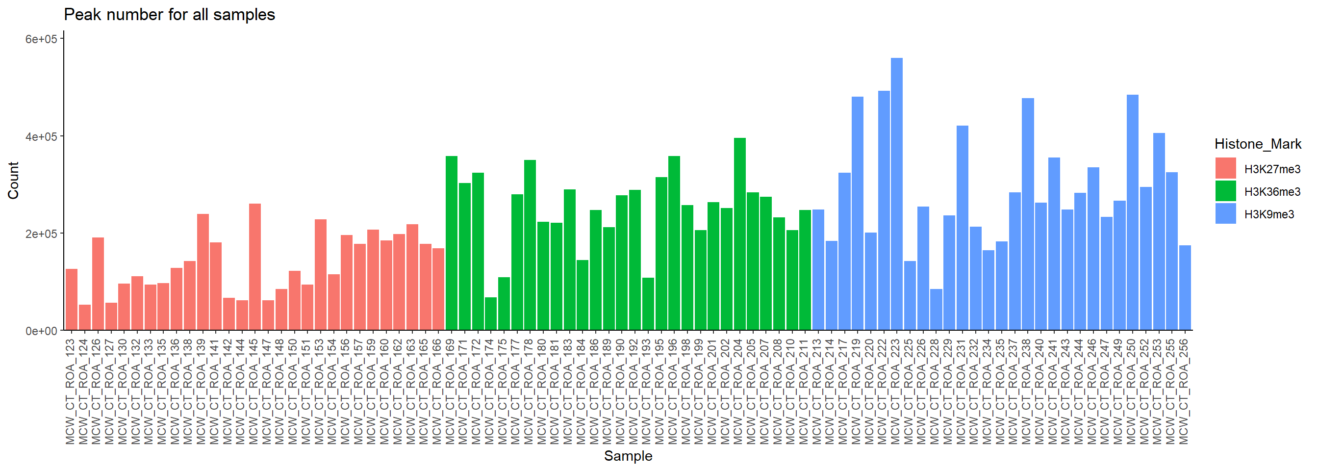

Version	Author	Date
3c5800a	infurnoheat	2025-07-22

all_peak_var %>% 
  ggplot(., aes (x=Histone_Mark, y = Count, fill = Histone_Mark))+
  geom_boxplot()+
   ylab("Count")+
   theme_classic()+
  # facet_wrap(~histone)+
  ggtitle("Peak count across histones")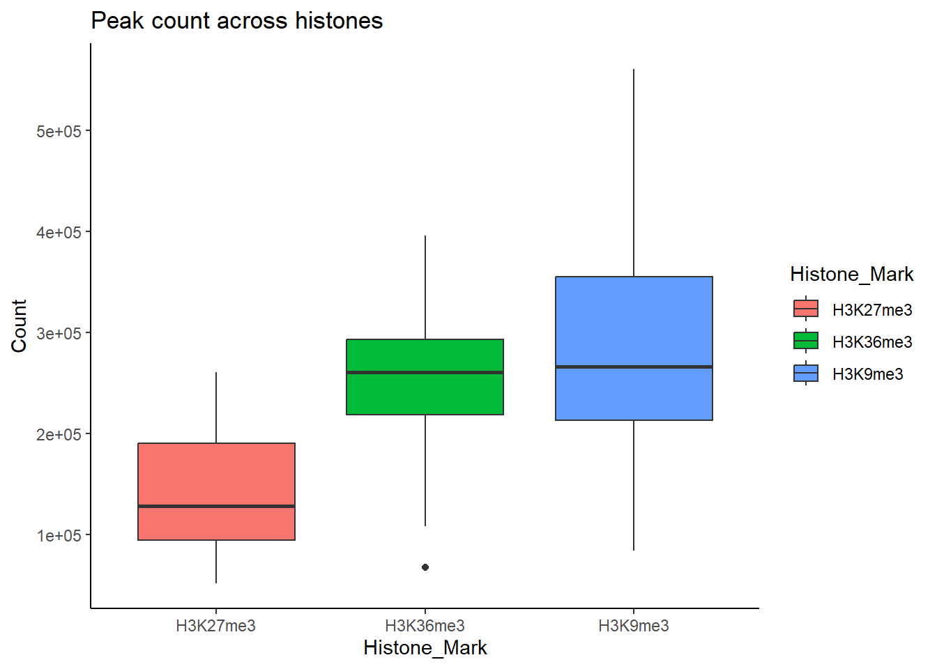

Version	Author	Date
3c5800a	infurnoheat	2025-07-22

all_peak_var %>% 
  ggplot(., aes (x=Treatment, y = Count, fill = Histone_Mark))+
  geom_boxplot()+
   ylab("Count")+
   theme_classic()+
  # facet_wrap(~histone)+
  ggtitle("Peak count across histones")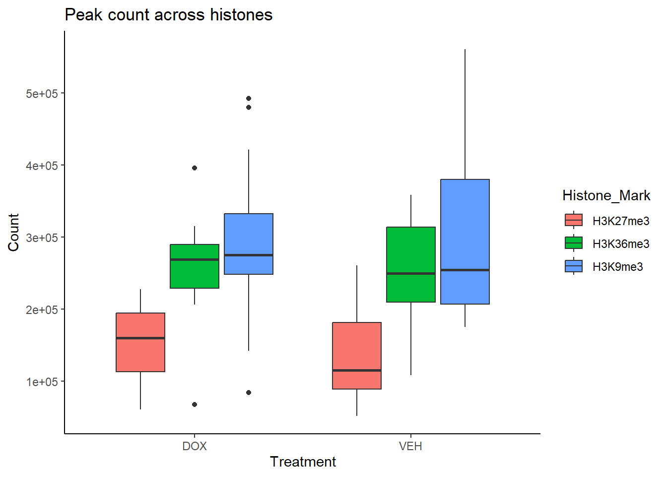

Version	Author	Date
3c5800a	infurnoheat	2025-07-22

all_peak_var %>% 
  ggplot(., aes (x=Timepoint, y = Count, fill = Histone_Mark))+
  geom_boxplot()+
   ylab("Count")+
   theme_classic()+
  # facet_wrap(~histone)+
  ggtitle("Peak count across histones")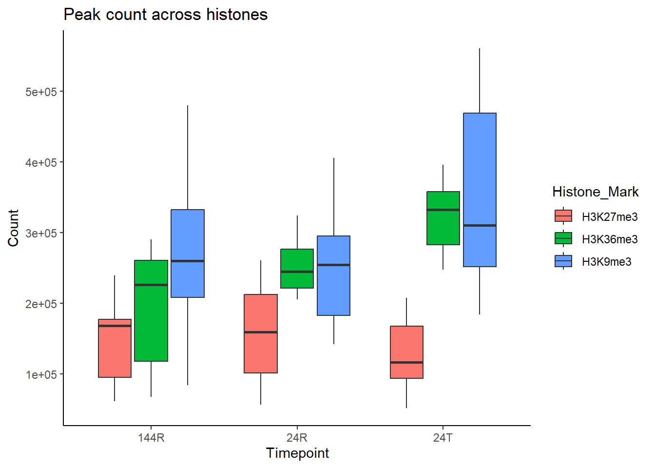

Version	Author	Date
3c5800a	infurnoheat	2025-07-22

Peak Calling for Q=0.01 and Broad=0.5 with No Lambda

Data Initialization

peak_ct <- read_delim("data/peaks/peaks_cts_nlq1e2b5e1.txt", delim = "\t")
H3K27ac_peaks <- read_delim("data/peaks/H3K27ac_final_results.tsv",delim = "\t")
H3K27me3_peaks <- read_delim("data/peaks/H3K27me3_nlq1e2b5e1_results.tsv",delim = "\t")
H3K36me3_peaks <- read_delim("data/peaks/H3K36me3_nlq1e2b5e1_results.tsv",delim = "\t")
H3K9me3_peaks <- read_delim("data/peaks/H3K9me3_nlq1e2b5e1_results.tsv",delim = "\t")

all_peak_var <- rbind(H3K27ac_peaks, H3K27me3_peaks, H3K36me3_peaks, H3K9me3_peaks)

all_peak_var <- all_peak_var %>%
  dplyr::select(Sample, Total_Reads, Fragments, Reads_in_Peaks, FRiP) %>%
  left_join(.,sampleinfo, by=c("Sample"="Library ID")) %>%
  left_join(.,peak_ct, by=c("Sample"="Sample"))
all_peak_var <- all_peak[(!all_peak$Treatment %in% "5FU"),]
all_peak_var <- all_peak_var[(!all_peak_var$Histone_Mark %in% "H3K27ac"),]

Peak Visualization

all_peak_var %>% 
   ggplot(.,aes(x=Sample, y=Count,fill=Histone_Mark))+
   geom_col()+
   ylab("Counts")+
   theme_classic()+
  # facet_wrap(~histone)+
  ggtitle("Peak number for all samples")+ 
  theme(axis.text.x=element_text(vjust = .2,angle=90))+
  scale_y_continuous( expand = expansion(mult = c(0, .1)))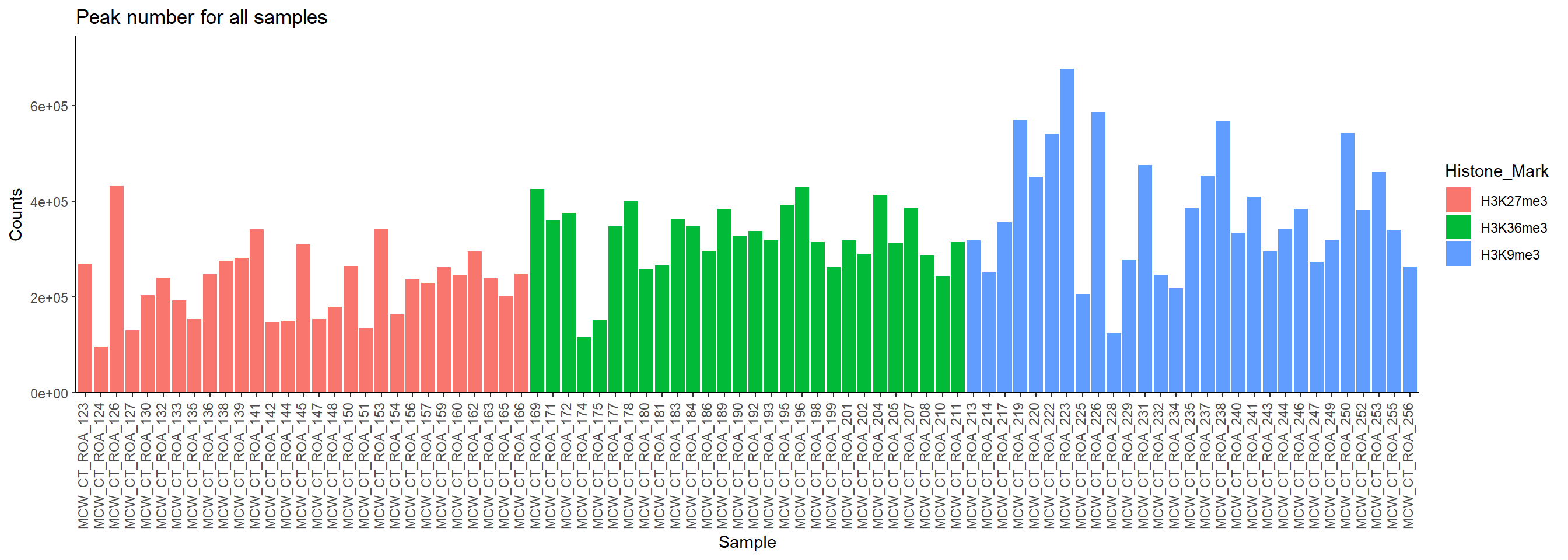

Version	Author	Date
3c5800a	infurnoheat	2025-07-22

all_peak_var %>% 
  ggplot(., aes (x=Histone_Mark, y = Count, fill = Histone_Mark))+
  geom_boxplot()+
   ylab("Count")+
   theme_classic()+
  # facet_wrap(~histone)+
  ggtitle("Peak count across histones")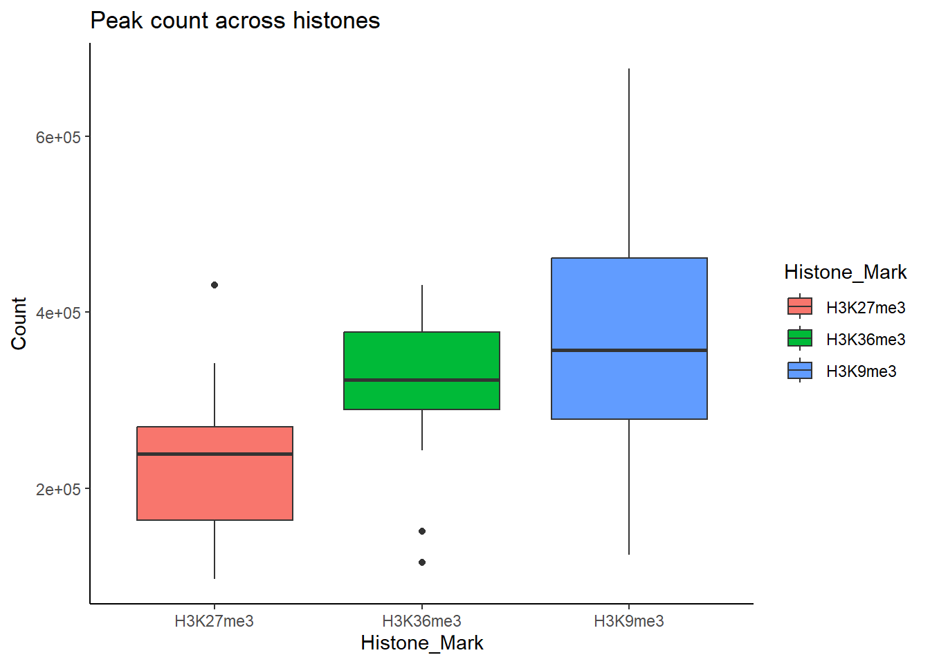

Version	Author	Date
3c5800a	infurnoheat	2025-07-22

all_peak_var %>% 
  ggplot(., aes (x=Treatment, y = Count, fill = Histone_Mark))+
  geom_boxplot()+
   ylab("Count")+
   theme_classic()+
  # facet_wrap(~histone)+
  ggtitle("Peak count across histones")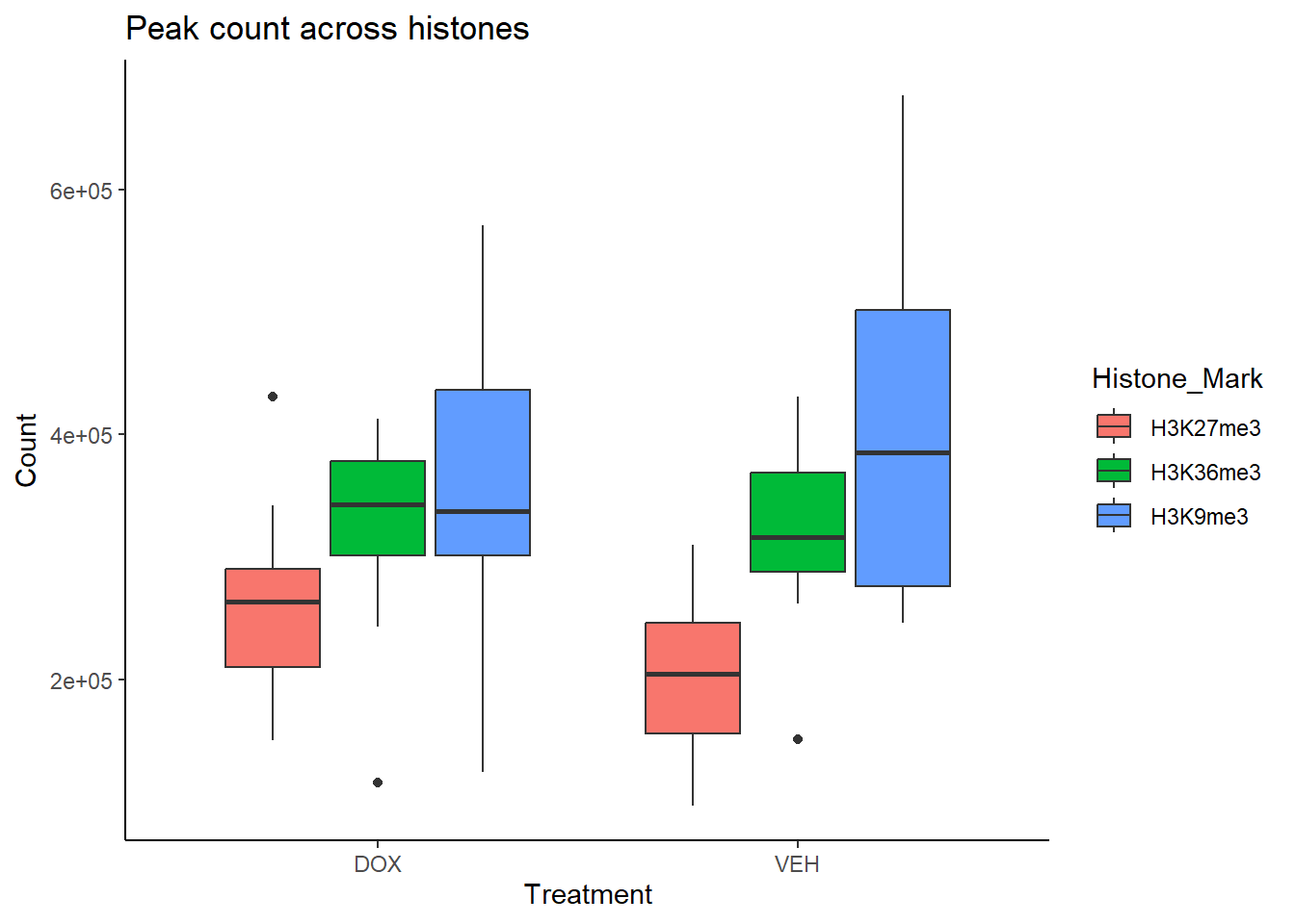

Version	Author	Date
3c5800a	infurnoheat	2025-07-22

all_peak_var %>% 
  ggplot(., aes (x=Timepoint, y = Count, fill = Histone_Mark))+
  geom_boxplot()+
   ylab("Count")+
   theme_classic()+
  # facet_wrap(~histone)+
  ggtitle("Peak count across histones")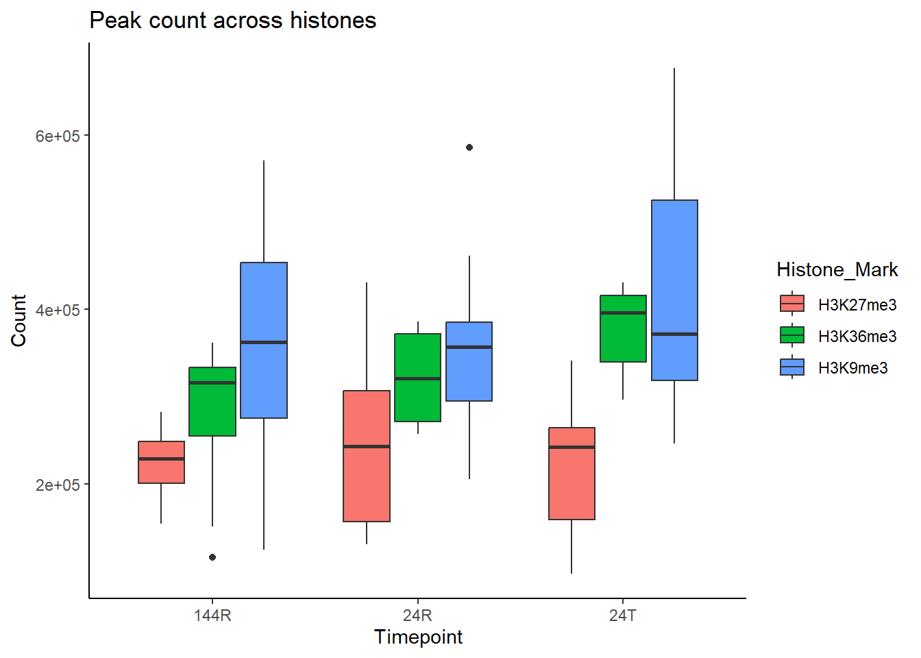

Version	Author	Date
3c5800a	infurnoheat	2025-07-22

Peak Calling for Q=0.01 and Broad=0.5 with Lambda

Data Initialization

peak_ct_var <- read_delim("data/peaks/peaks_cts_lq1e2b5e1.txt", delim = "\t")
H3K27ac_peaks <- read_delim("data/peaks/H3K27ac_final_results.tsv",delim = "\t")
H3K27me3_peaks <- read_delim("data/peaks/H3K27me3_lq1e2b5e1_results.tsv",delim = "\t")
H3K36me3_peaks <- read_delim("data/peaks/H3K36me3_lq1e2b5e1_results.tsv",delim = "\t")
H3K9me3_peaks <- read_delim("data/peaks/H3K9me3_lq1e2b5e1_results.tsv",delim = "\t")

all_peak_var <- rbind(H3K27ac_peaks, H3K27me3_peaks, H3K36me3_peaks, H3K9me3_peaks)

all_peak_var <- all_peak_var %>%
  dplyr::select(Sample, Total_Reads, Fragments, Reads_in_Peaks, FRiP) %>%
  left_join(.,sampleinfo, by=c("Sample"="Library ID")) %>%
  left_join(.,peak_ct, by=c("Sample"="Sample"))
all_peak_var <- all_peak_var[(!all_peak_var$Treatment %in% "5FU"),]
all_peak_var <- all_peak_var[(!all_peak_var$Histone_Mark %in% "H3K27ac"),]

Peak Visualization

all_peak_var %>% 
   ggplot(.,aes(x=Sample, y=Count,fill=Histone_Mark))+
   geom_col()+
   ylab("Count")+
   theme_classic()+
  # facet_wrap(~histone)+
  ggtitle("Peak number for all samples")+ 
  theme(axis.text.x=element_text(vjust = .2,angle=90))+
  scale_y_continuous( expand = expansion(mult = c(0, .1)))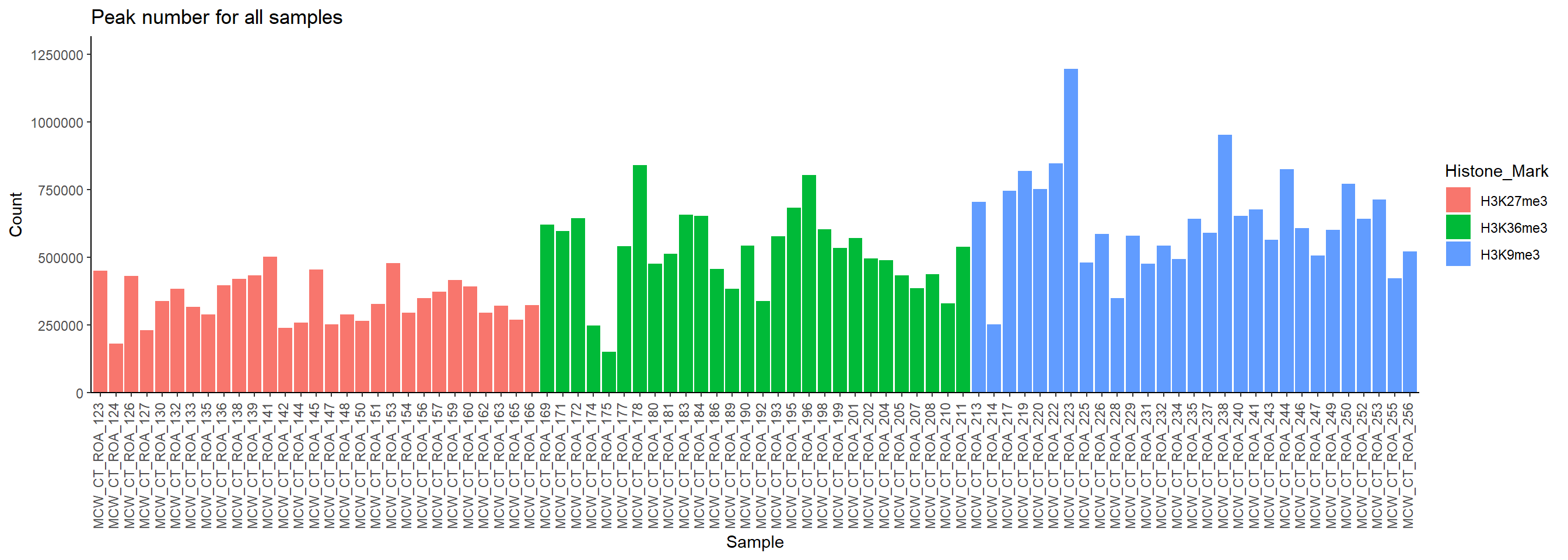

Version	Author	Date
3c5800a	infurnoheat	2025-07-22

all_peak_var %>% 
  ggplot(., aes (x=Histone_Mark, y = Count, fill = Histone_Mark))+
  geom_boxplot()+
   ylab("Count")+
   theme_classic()+
  # facet_wrap(~histone)+
  ggtitle("Peak count across histones")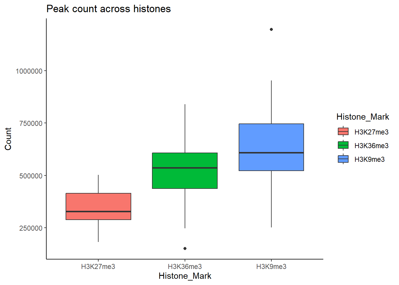

Version	Author	Date
3c5800a	infurnoheat	2025-07-22

all_peak_var %>% 
  ggplot(., aes (x=Treatment, y = Count, fill = Histone_Mark))+
  geom_boxplot()+
   ylab("Count")+
   theme_classic()+
  # facet_wrap(~histone)+
  ggtitle("Peak count across histones")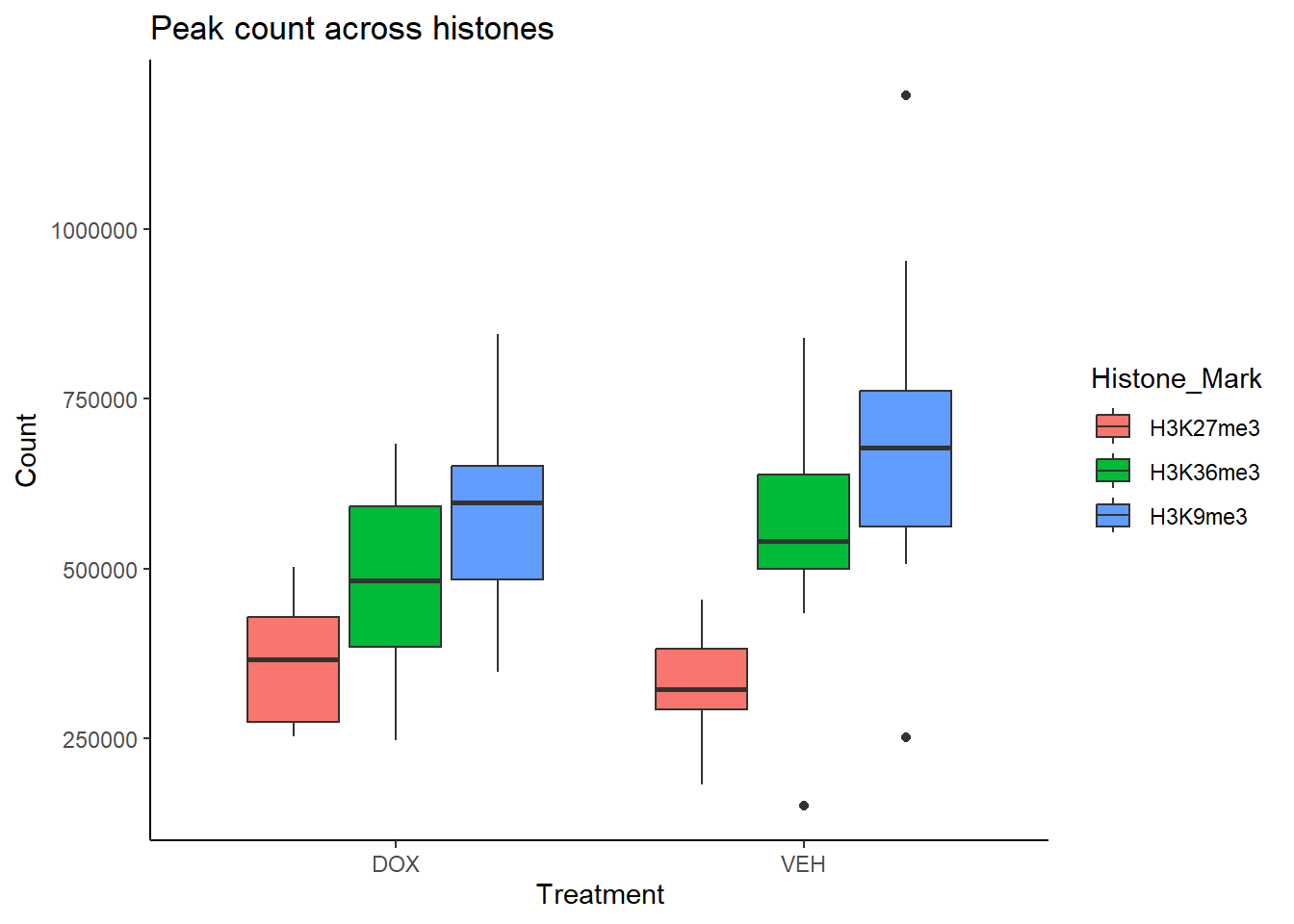

Version	Author	Date
3c5800a	infurnoheat	2025-07-22

all_peak_var %>% 
  ggplot(., aes (x=Timepoint, y = Count, fill = Histone_Mark))+
  geom_boxplot()+
   ylab("Count")+
   theme_classic()+
  # facet_wrap(~histone)+
  ggtitle("Peak count across histones")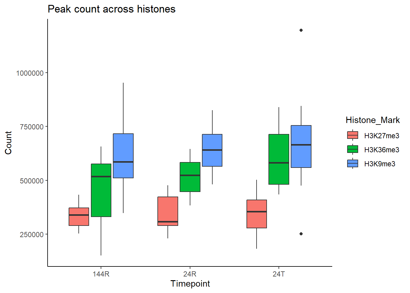

Version	Author	Date
3c5800a	infurnoheat	2025-07-22

Peak Calling for Q=0.005 and Broad=0.01 with No Lambda

Data Initialization

peak_ct <- read_delim("data/peaks/peaks_cts_nlq5e3b1e2.txt", delim = "\t")
H3K27ac_peaks <- read_delim("data/peaks/H3K27ac_final_results.tsv",delim = "\t")
H3K27me3_peaks <- read_delim("data/peaks/H3K27me3_nlq5e3b1e2_results.tsv",delim = "\t")
H3K36me3_peaks <- read_delim("data/peaks/H3K36me3_nlq5e3b1e2_results.tsv",delim = "\t")
H3K9me3_peaks <- read_delim("data/peaks/H3K9me3_nlq5e3b1e2_results.tsv",delim = "\t")

all_peak_var <- rbind(H3K27ac_peaks, H3K27me3_peaks, H3K36me3_peaks, H3K9me3_peaks)

all_peak_var <- all_peak_var %>%
  dplyr::select(Sample, Total_Reads, Fragments, Reads_in_Peaks, FRiP) %>%
  left_join(.,sampleinfo, by=c("Sample"="Library ID")) %>%
  left_join(.,peak_ct, by=c("Sample"="Sample"))
all_peak_var <- all_peak_var[(!all_peak_var$Treatment %in% "5FU"),]
all_peak_var <- all_peak_var[(!all_peak_var$Histone_Mark %in% "H3K27ac"),]

Peak Visualization

all_peak_var %>% 
   ggplot(.,aes(x=Sample, y=Count,fill=Histone_Mark))+
   geom_col()+
   ylab("Count")+
   theme_classic()+
  # facet_wrap(~histone)+
  ggtitle("Peak number for all samples")+ 
  theme(axis.text.x=element_text(vjust = .2,angle=90))+
  scale_y_continuous( expand = expansion(mult = c(0, .1)))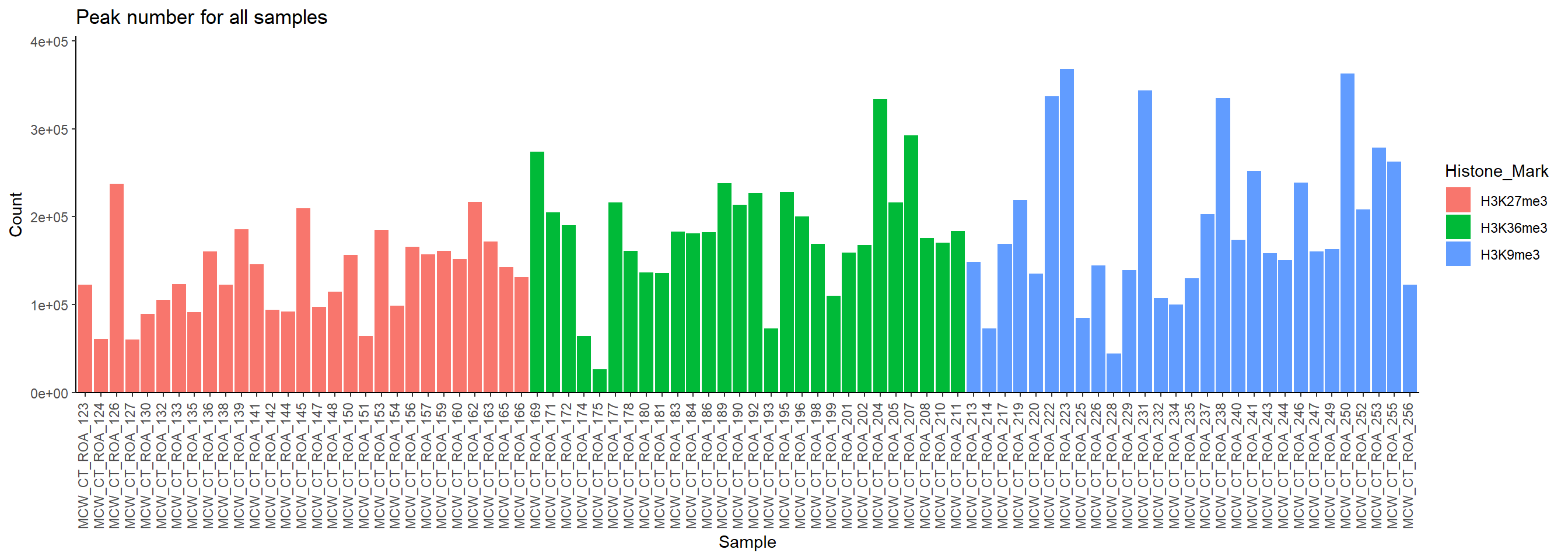

Version	Author	Date
3c5800a	infurnoheat	2025-07-22

all_peak_var %>% 
  ggplot(., aes (x=Histone_Mark, y = Count, fill = Histone_Mark))+
  geom_boxplot()+
   ylab("Count")+
   theme_classic()+
  # facet_wrap(~histone)+
  ggtitle("Peak count across histones")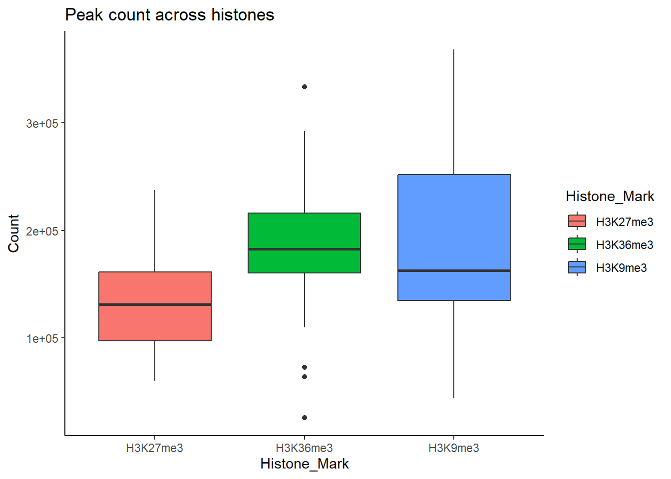

Version	Author	Date
3c5800a	infurnoheat	2025-07-22

all_peak_var %>% 
  ggplot(., aes (x=Treatment, y = Count, fill = Histone_Mark))+
  geom_boxplot()+
   ylab("Count")+
   theme_classic()+
  # facet_wrap(~histone)+
  ggtitle("Peak count across histones")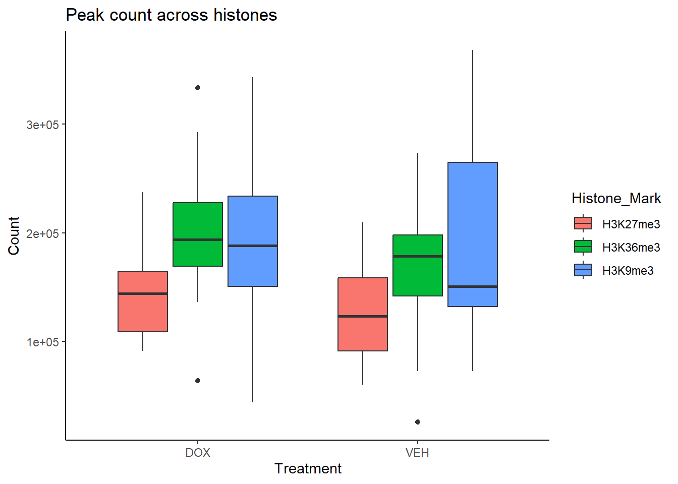

Version	Author	Date
3c5800a	infurnoheat	2025-07-22

all_peak_var %>% 
  ggplot(., aes (x=Timepoint, y = Count, fill = Histone_Mark))+
  geom_boxplot()+
   ylab("Count")+
   theme_classic()+
  # facet_wrap(~histone)+
  ggtitle("Peak count across histones")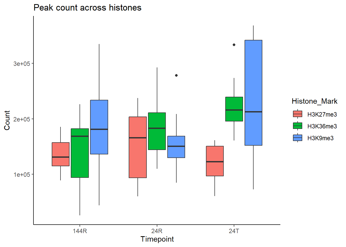

Version	Author	Date
3c5800a	infurnoheat	2025-07-22

Peak Calling for Q=0.005 and Broad=0.01 with Lambda

Data Initialization

peak_ct <- read_delim("data/peaks/peaks_cts_lq5e3b1e2.txt", delim = "\t")
H3K27ac_peaks <- read_delim("data/peaks/H3K27ac_final_results.tsv",delim = "\t")
H3K27me3_peaks <- read_delim("data/peaks/H3K27me3_lq5e3b1e2_results.tsv",delim = "\t")
H3K36me3_peaks <- read_delim("data/peaks/H3K36me3_lq5e3b1e2_results.tsv",delim = "\t")
H3K9me3_peaks <- read_delim("data/peaks/H3K9me3_lq5e3b1e2_results.tsv",delim = "\t")

all_peak_var <- rbind(H3K27ac_peaks, H3K27me3_peaks, H3K36me3_peaks, H3K9me3_peaks)

all_peak_var <- all_peak_var %>%
  dplyr::select(Sample, Total_Reads, Fragments, Reads_in_Peaks, FRiP) %>%
  left_join(.,sampleinfo, by=c("Sample"="Library ID")) %>%
  left_join(.,peak_ct, by=c("Sample"="Sample"))
all_peak_var <- all_peak_var[(!all_peak_var$Treatment %in% "5FU"),]
all_peak_var <- all_peak_var[(!all_peak_var$Histone_Mark %in% "H3K27ac"),]

Peak Visualization

all_peak_var %>% 
   ggplot(.,aes(x=Sample, y=Count,fill=Histone_Mark))+
   geom_col()+
   ylab("Count")+
   theme_classic()+
  # facet_wrap(~histone)+
  ggtitle("Peak number for all samples")+ 
  theme(axis.text.x=element_text(vjust = .2,angle=90))+
  scale_y_continuous( expand = expansion(mult = c(0, .1)))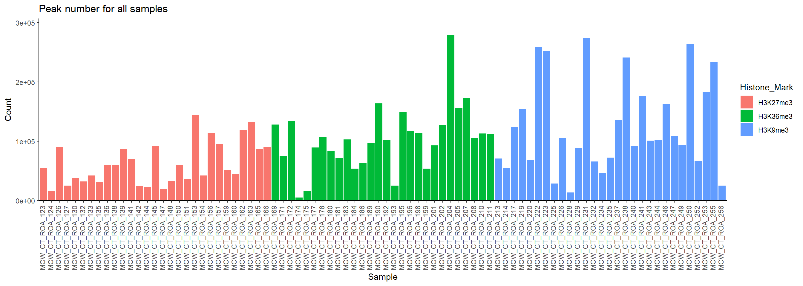

Version	Author	Date
3c5800a	infurnoheat	2025-07-22

all_peak_var %>% 
  ggplot(., aes (x=Histone_Mark, y = Count, fill = Histone_Mark))+
  geom_boxplot()+
   ylab("Count")+
   theme_classic()+
  # facet_wrap(~histone)+
  ggtitle("Peak count across histones")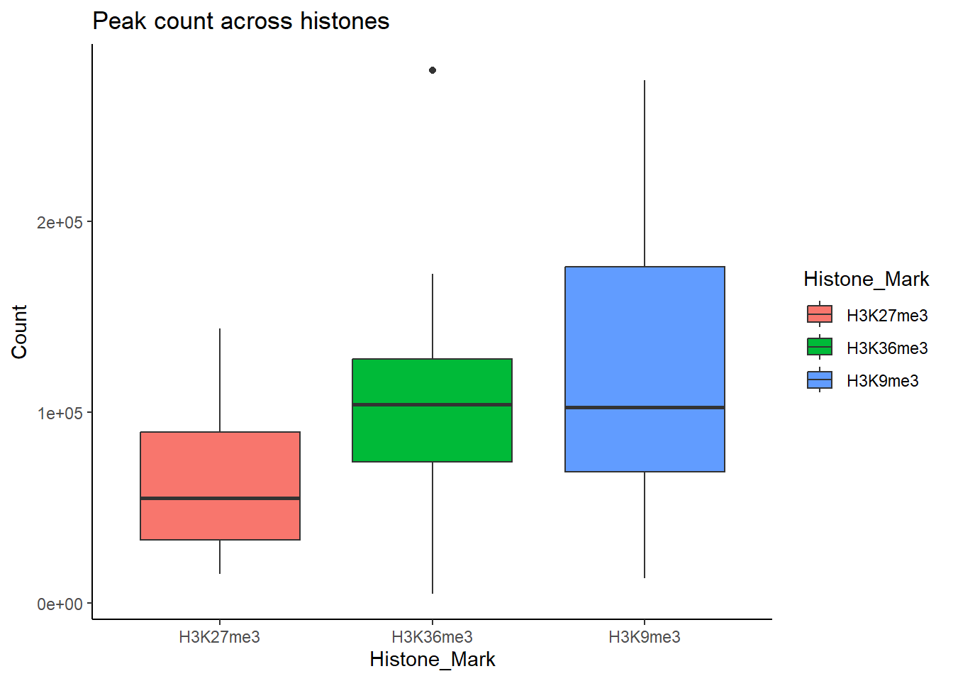

Version	Author	Date
3c5800a	infurnoheat	2025-07-22

all_peak_var %>% 
  ggplot(., aes (x=Treatment, y = Count, fill = Histone_Mark))+
  geom_boxplot()+
   ylab("Count")+
   theme_classic()+
  # facet_wrap(~histone)+
  ggtitle("Peak count across histones")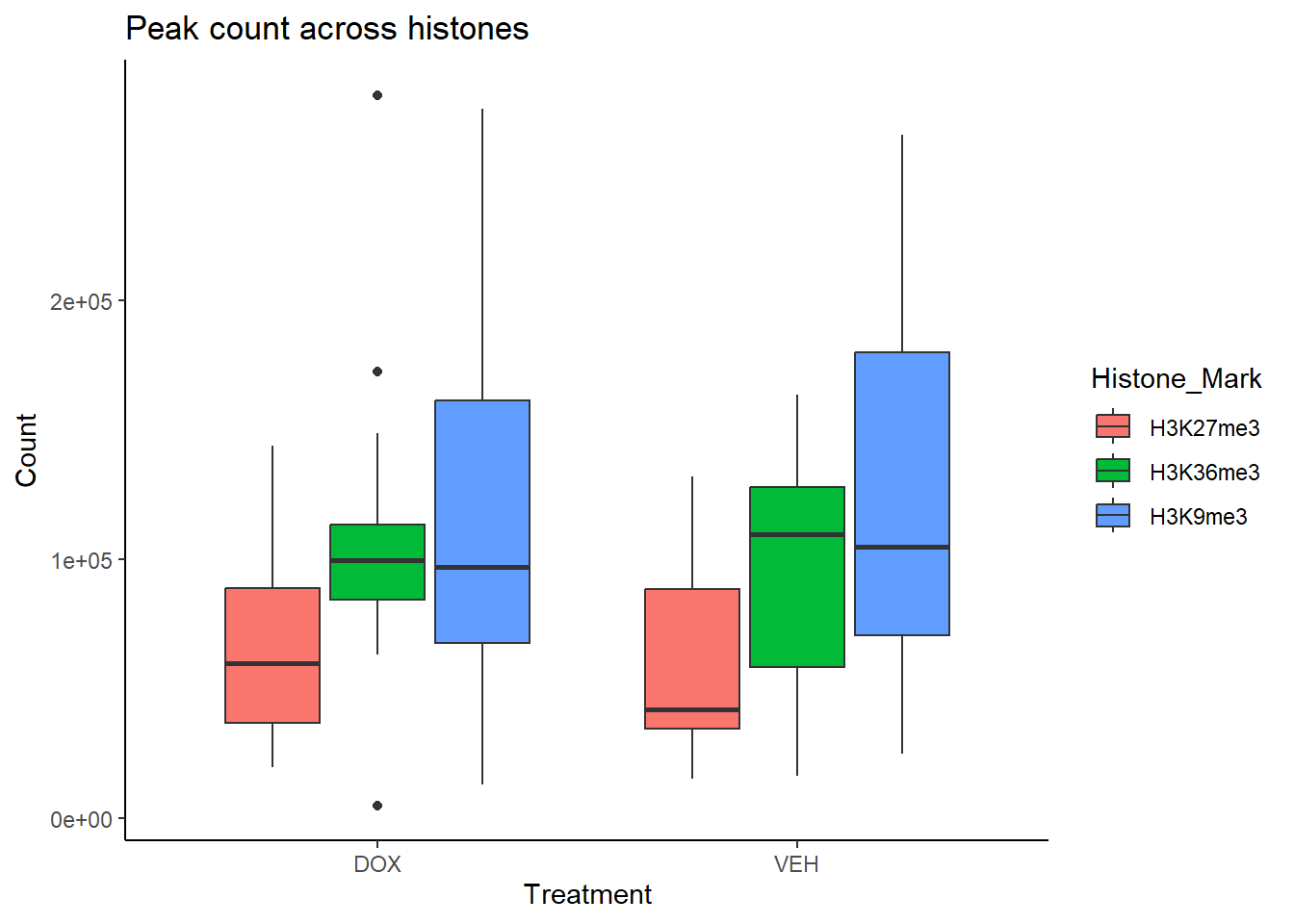

Version	Author	Date
3c5800a	infurnoheat	2025-07-22

all_peak_var %>% 
  ggplot(., aes (x=Timepoint, y = Count, fill = Histone_Mark))+
  geom_boxplot()+
   ylab("Count")+
   theme_classic()+
  # facet_wrap(~histone)+
  ggtitle("Peak count across histones")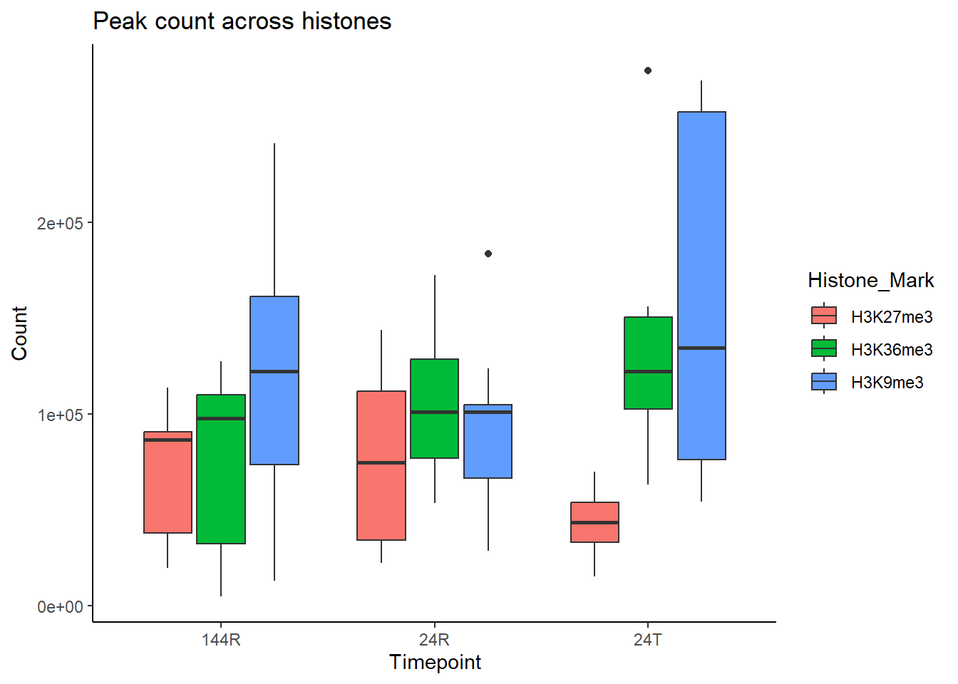

Version	Author	Date
3c5800a	infurnoheat	2025-07-22

Picard with Broad Peaks

peak_ct <- read_delim("data/peaks/peaks_cts_picard_broad.txt", delim = "\t")
H3K27ac_peaks <- read_delim("data/peaks/H3K27ac_picard_results.tsv",delim = "\t")
H3K27me3_peaks <- read_delim("data/peaks/H3K27me3_picard_broad_results.tsv",delim = "\t")
H3K36me3_peaks <- read_delim("data/peaks/H3K36me3_picard_broad_results.tsv",delim = "\t")
H3K9me3_peaks <- read_delim("data/peaks/H3K9me3_picard_broad_results.tsv",delim = "\t")

all_peak_pb <- rbind(H3K27ac_peaks, H3K27me3_peaks, H3K36me3_peaks, H3K9me3_peaks)

all_peak_pb <- all_peak_pb %>%
  dplyr::select(Sample, Total_Reads, Fragments, Reads_in_Peaks, FRiP) %>%
  left_join(.,sampleinfo, by=c("Sample"="Library ID")) %>%
  left_join(.,peak_ct, by=c("Sample"="Sample"))
all_peak_pb <- all_peak_pb[(!all_peak_pb$Treatment %in% "5FU"),]

all_peak_pb %>% 
   ggplot(.,aes(x=Sample, y=Count,fill=Histone_Mark))+
   geom_col()+
   ylab("Count")+
   theme_classic()+
  # facet_wrap(~histone)+
  ggtitle("Peak number for all samples")+ 
  theme(axis.text.x=element_text(vjust = .2,angle=90))+
  scale_y_continuous( expand = expansion(mult = c(0, .1)))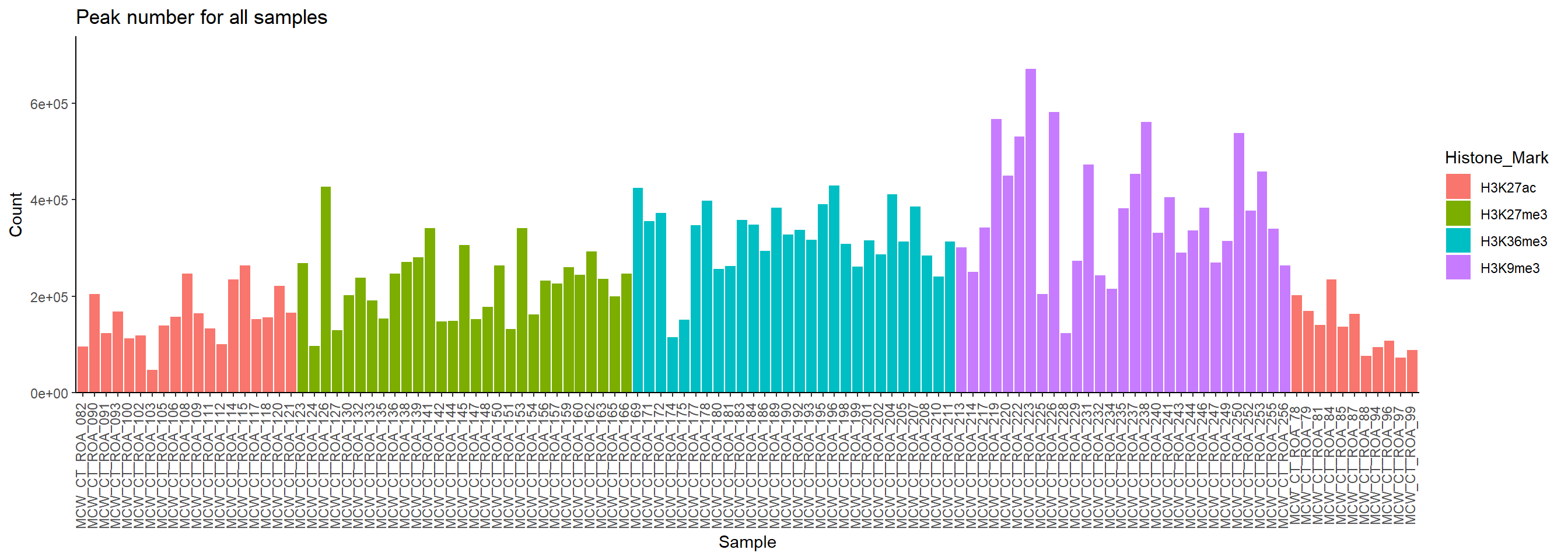

all_peak_pb %>% 
  ggplot(., aes (x=Histone_Mark, y = Count, fill = Histone_Mark))+
  geom_boxplot()+
   ylab("Count")+
   theme_classic()+
  # facet_wrap(~histone)+
  ggtitle("Peak count across histones")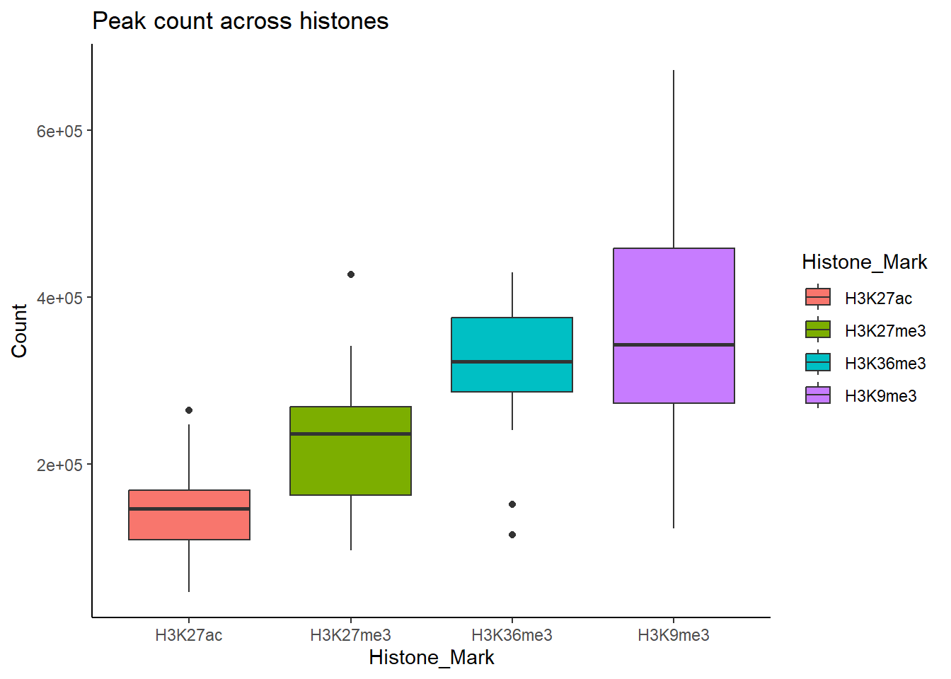

all_peak_pb %>% 
  ggplot(., aes (x=Treatment, y = Count, fill = Histone_Mark))+
  geom_boxplot()+
   ylab("Count")+
   theme_classic()+
  # facet_wrap(~histone)+
  ggtitle("Peak count across histones")

all_peak_pb %>% 
  ggplot(., aes (x=Timepoint, y = Count, fill = Histone_Mark))+
  geom_boxplot()+
   ylab("Count")+
   theme_classic()+
  # facet_wrap(~histone)+
  ggtitle("Peak count across histones")

Picard with Broad as Narrow Peaks

peak_ct <- read_delim("data/peaks/peaks_cts_picard_narrow.txt", delim = "\t")
H3K27ac_peaks <- read_delim("data/peaks/H3K27ac_picard_results.tsv",delim = "\t")
H3K27me3_peaks <- read_delim("data/peaks/H3K27me3_picard_narrow_results.tsv",delim = "\t")
H3K36me3_peaks <- read_delim("data/peaks/H3K36me3_picard_narrow_results.tsv",delim = "\t")
H3K9me3_peaks <- read_delim("data/peaks/H3K9me3_picard_narrow_results.tsv",delim = "\t")

all_peak_pn <- rbind(H3K27ac_peaks, H3K27me3_peaks, H3K36me3_peaks, H3K9me3_peaks)

all_peak_pn <- all_peak_pn %>%
  dplyr::select(Sample, Total_Reads, Fragments, Reads_in_Peaks, FRiP) %>%
  left_join(.,sampleinfo, by=c("Sample"="Library ID")) %>%
  left_join(.,peak_ct, by=c("Sample"="Sample"))
all_peak_pn <- all_peak_pn[(!all_peak_pn$Treatment %in% "5FU"),]

all_peak_pn %>% 
   ggplot(.,aes(x=Sample, y=Count,fill=Histone_Mark))+
   geom_col()+
   ylab("Count")+
   theme_classic()+
  # facet_wrap(~histone)+
  ggtitle("Peak number for all samples")+ 
  theme(axis.text.x=element_text(vjust = .2,angle=90))+
  scale_y_continuous( expand = expansion(mult = c(0, .1)))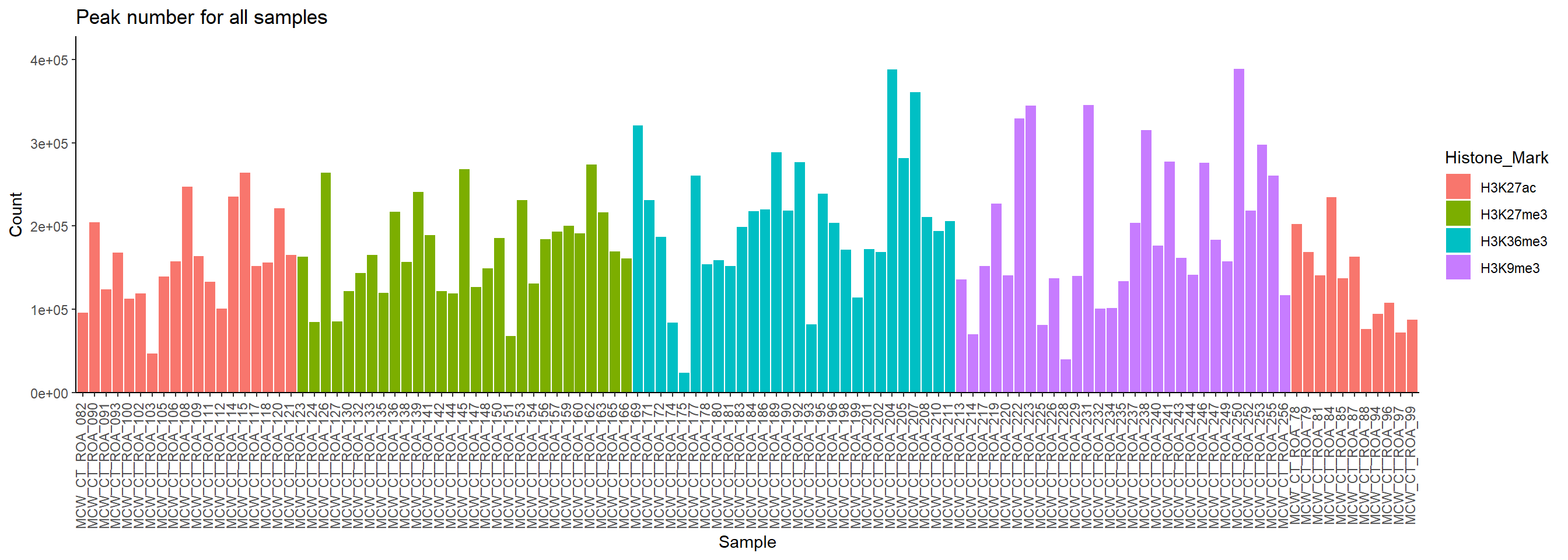

all_peak_pn %>% 
  ggplot(., aes (x=Histone_Mark, y = Count, fill = Histone_Mark))+
  geom_boxplot()+
   ylab("Count")+
   theme_classic()+
  # facet_wrap(~histone)+
  ggtitle("Peak count across histones")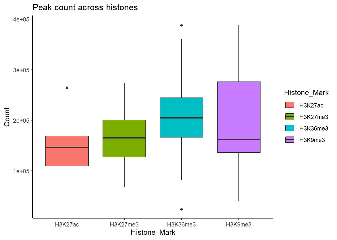

all_peak_pn %>% 
  ggplot(., aes (x=Treatment, y = Count, fill = Histone_Mark))+
  geom_boxplot()+
   ylab("Count")+
   theme_classic()+
  # facet_wrap(~histone)+
  ggtitle("Peak count across histones")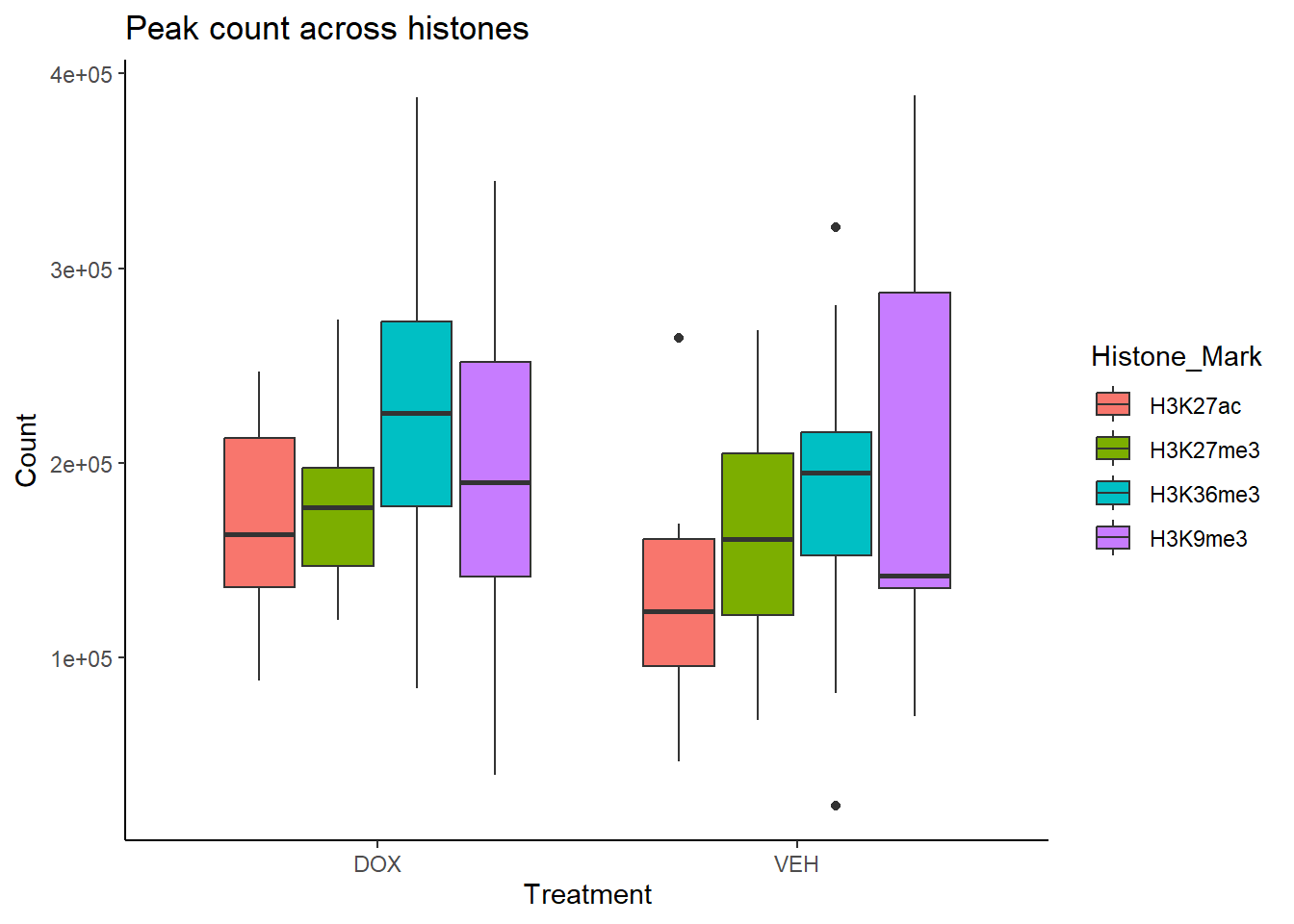

all_peak_pn %>% 
  ggplot(., aes (x=Timepoint, y = Count, fill = Histone_Mark))+
  geom_boxplot()+
   ylab("Count")+
   theme_classic()+
  # facet_wrap(~histone)+
  ggtitle("Peak count across histones")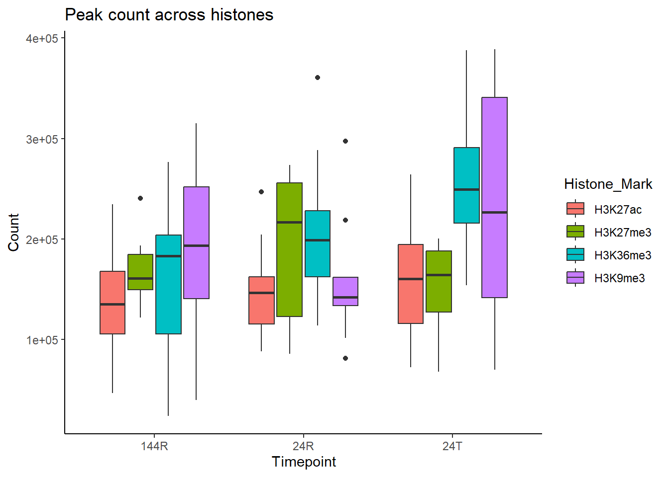

Picard with Broad as Stringent Narrow Peaks

peak_ct <- read_delim("data/peaks/peaks_cts_1e3_narrow.txt", delim = "\t")
H3K27ac_peaks <- read_delim("data/peaks/H3K27ac_picard_results.tsv",delim = "\t")
H3K27me3_peaks <- read_delim("data/peaks/H3K27me3_1e3_narrow_results.tsv",delim = "\t")
H3K36me3_peaks <- read_delim("data/peaks/H3K36me3_1e3_narrow_results.tsv",delim = "\t")
H3K9me3_peaks <- read_delim("data/peaks/H3K9me3_1e3_narrow_results.tsv",delim = "\t")

all_peak_sn <- rbind(H3K27ac_peaks, H3K27me3_peaks, H3K36me3_peaks, H3K9me3_peaks)

all_peak_sn <- all_peak_sn %>%
  dplyr::select(Sample, Total_Reads, Fragments, Reads_in_Peaks, FRiP) %>%
  left_join(.,sampleinfo, by=c("Sample"="Library ID")) %>%
  left_join(.,peak_ct, by=c("Sample"="Sample"))
all_peak_sn <- all_peak_sn[(!all_peak_sn$Treatment %in% "5FU"),]

all_peak_sn %>% 
   ggplot(.,aes(x=Sample, y=Count,fill=Histone_Mark))+
   geom_col()+
   ylab("Count")+
   theme_classic()+
  # facet_wrap(~histone)+
  ggtitle("Peak number for all samples")+ 
  theme(axis.text.x=element_text(vjust = .2,angle=90))+
  scale_y_continuous( expand = expansion(mult = c(0, .1)))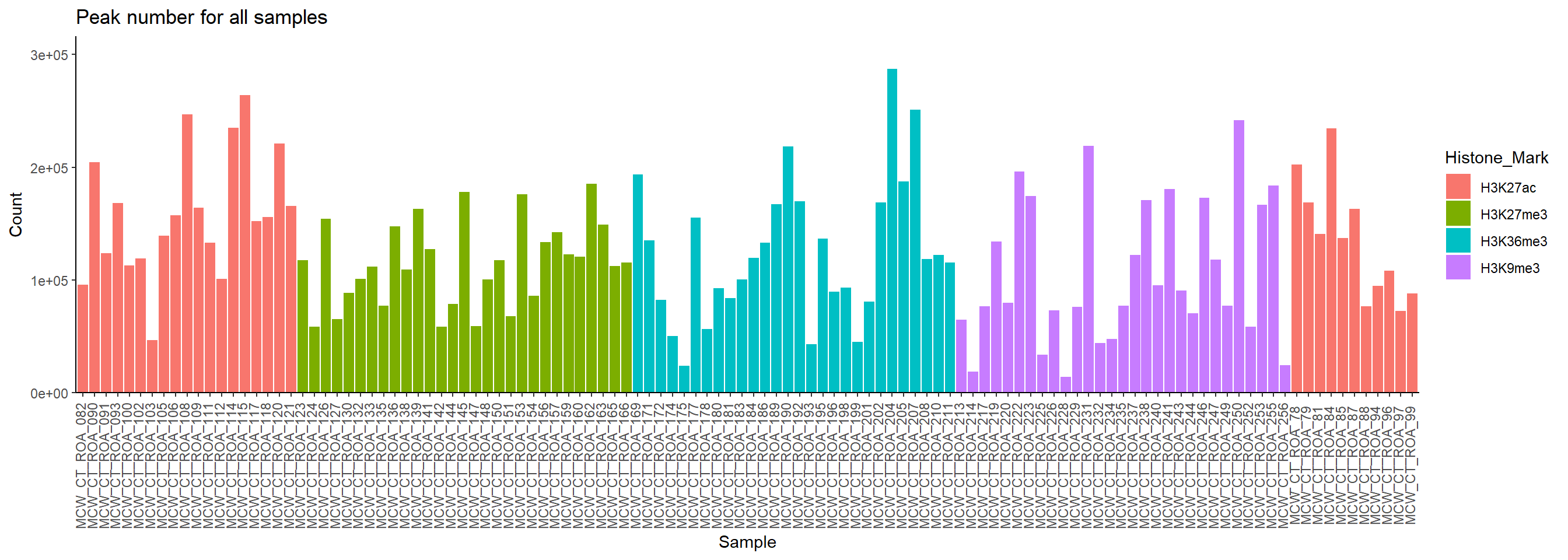

all_peak_sn %>% 
  ggplot(., aes (x=Histone_Mark, y = Count, fill = Histone_Mark))+
  geom_boxplot()+
   ylab("Count")+
   theme_classic()+
  # facet_wrap(~histone)+
  ggtitle("Peak count across histones")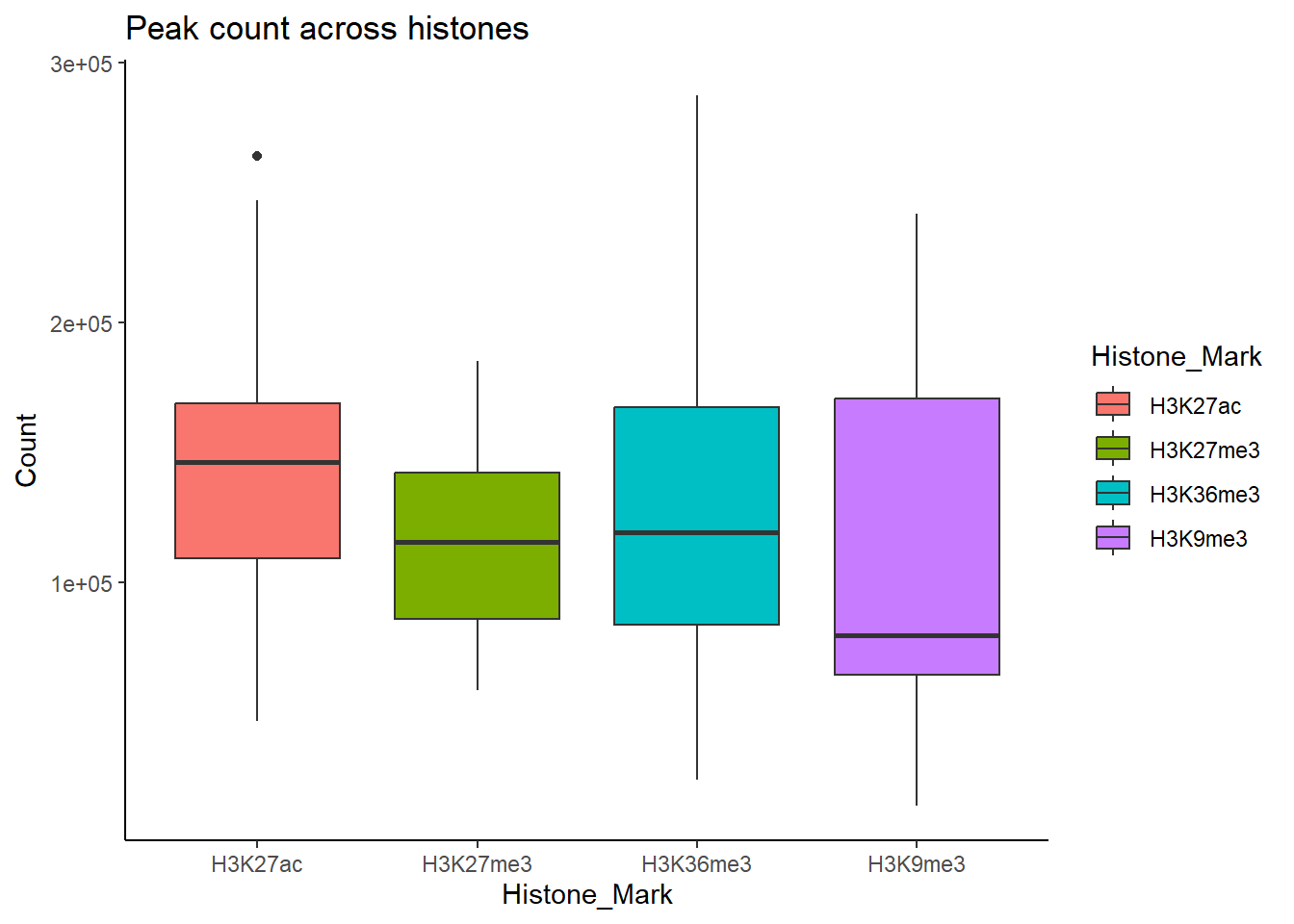

all_peak_sn %>% 
  ggplot(., aes (x=Treatment, y = Count, fill = Histone_Mark))+
  geom_boxplot()+
   ylab("Count")+
   theme_classic()+
  # facet_wrap(~histone)+
  ggtitle("Peak count across histones")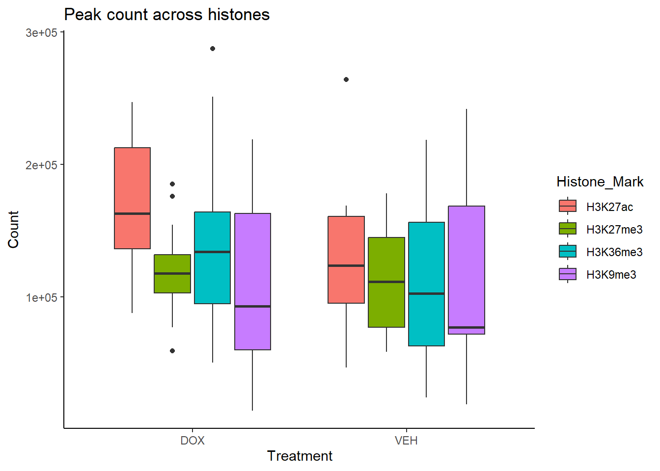

all_peak_sn %>% 
  ggplot(., aes (x=Timepoint, y = Count, fill = Histone_Mark))+
  geom_boxplot()+
   ylab("Count")+
   theme_classic()+
  # facet_wrap(~histone)+
  ggtitle("Peak count across histones")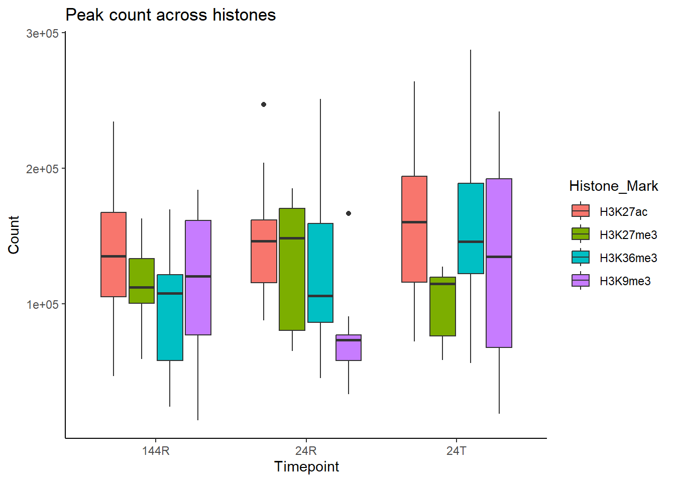

Tagging Questionable Libraries by FRiP

questionable_frip = all_peak[(all_peak$FRiP < 0.02),]
questionable_frip

# A tibble: 0 × 10
# ℹ 10 variables: Sample <chr>, Total_Reads <dbl>, Fragments <dbl>,
#   Reads_in_Peaks <dbl>, FRiP <dbl>, Histone_Mark <chr>, Individual <chr>,
#   Treatment <chr>, Timepoint <chr>, Count <dbl>

Peak Widths

Peak Width Function

histone_list <- c("H3K27ac", "H3K27me3", "H3K9me3", "H3K36me3")
get_peak_widths_long_split <- function(histone, var) {
  path <- file.path("data/peaks", histone)
  if (histone == "H3K27ac"){
    file_list = list.files(path = path, pattern = paste0("picard_peaks.narrowPeak$", sep=""), full.names = TRUE)
  } else {
    file_list = list.files(path = path, pattern = paste0(var,"_peaks.(narrowPeak|broadPeak)$", sep=""), full.names = TRUE)
  }
  process_peak <- function(file_path, label) {
    filename <- basename(file_path)
    peak_df <- fread(file_path, header = FALSE) %>%
      transmute(
        row = row_number(),
        width = abs(V3 - V2),
        file = paste0(histone, "-", filename),
        group = label
      )
    return(peak_df)
  }
  peak_list <- list(map(file_list, process_peak, label = var)) %>% flatten()
  bind_rows(peak_list)
}

Broad Visualization

all_peak_widths <- purrr::map_df(histone_list, get_peak_widths_long_split, var = "picard_broad")

anno_peak_width_long <- all_peak_widths %>% 
  mutate(file= gsub("_picard_broad_peaks.broadPeak","",file)) %>%
  separate_wider_delim(., cols=file, delim="-",names=c("histone","sample")) %>% 
  left_join(sampleinfo, by =c("sample"="Library ID"))

anno_peak_width_long %>%
  # distinct(histone)
  ggplot(.,aes(x=histone, y = width, fill = histone))+
  geom_violin()+
  # scale_fill_viridis_a(discrete = TRUE, begin = 0.1, end = 0.55, option = "magma", alpha = 0.8) +
  #   scale_color_viridis_a(discrete = TRUE, begin = 0.1, end = 0.9) +
    scale_y_continuous(trans = "log", breaks = c(400, 3000, 22000)) +
    theme_bw(base_size = 18) +
    ylab("Width of Peaks") +
    xlab("")+
  ggtitle("Width of all peaks with Broad Peaks")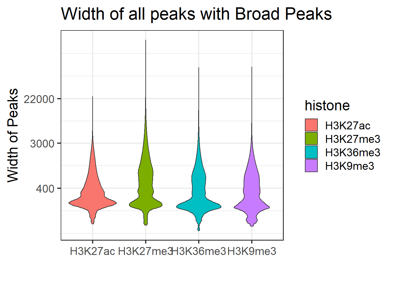

Broad as Narrow Visualization

all_peak_widths <- purrr::map_df(histone_list, get_peak_widths_long_split, var = "picard_narrow")

anno_peak_width_long <- all_peak_widths %>% 
  mutate(file= gsub("_picard_narrow_peaks.narrowPeak","",file)) %>%
  separate_wider_delim(., cols=file, delim="-",names=c("histone","sample")) %>% 
  left_join(sampleinfo, by =c("sample"="Library ID"))

anno_peak_width_long %>%
  # distinct(histone)
  ggplot(.,aes(x=histone, y = width, fill = histone))+
  geom_violin()+
  # scale_fill_viridis_a(discrete = TRUE, begin = 0.1, end = 0.55, option = "magma", alpha = 0.8) +
  #   scale_color_viridis_a(discrete = TRUE, begin = 0.1, end = 0.9) +
    scale_y_continuous(trans = "log", breaks = c(400, 3000, 22000)) +
    theme_bw(base_size = 18) +
    ylab("Width of Peaks") +
    xlab("")+
  ggtitle("Width of all peaks with Broad as Narrow")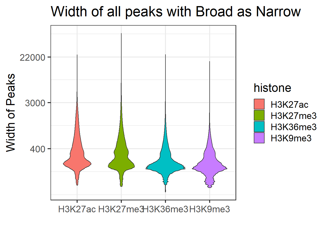

Broad as Narrow Stringent Visualization

all_peak_widths <- purrr::map_df(histone_list, get_peak_widths_long_split, var = "1e3_narrow")

anno_peak_width_long <- all_peak_widths %>% 
  mutate(file= gsub("_1e3_narrow_peaks.narrowPeak","",file)) %>%
  separate_wider_delim(., cols=file, delim="-",names=c("histone","sample")) %>% 
  left_join(sampleinfo, by =c("sample"="Library ID"))

anno_peak_width_long %>%
  # distinct(histone)
  ggplot(.,aes(x=histone, y = width, fill = histone))+
  geom_violin()+
  # scale_fill_viridis_a(discrete = TRUE, begin = 0.1, end = 0.55, option = "magma", alpha = 0.8) +
  #   scale_color_viridis_a(discrete = TRUE, begin = 0.1, end = 0.9) +
    scale_y_continuous(trans = "log", breaks = c(400, 3000, 22000)) +
    theme_bw(base_size = 18) +
    ylab("Width of Peaks") +
    xlab("")+
  ggtitle("Width of all peaks with Broad as Stringent Narrow")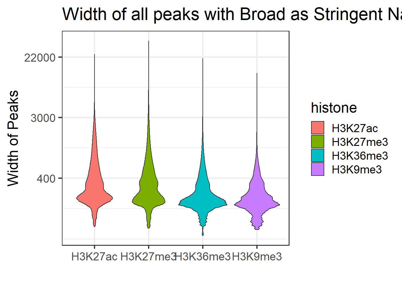

Feature Counts

featurects_merged <- read_delim("data/peaks/H3K27ac_merged_counts.txt", 
    delim = "\t", escape_double = FALSE, 
    trim_ws = TRUE, skip = 1)
featurects_cluster <- read_delim("data/peaks/H3K27ac_cluster_counts.txt", 
    delim = "\t", escape_double = FALSE, 
    trim_ws = TRUE, skip = 1)
featurects_iter <- read_delim("data/peaks/H3K27ac_iter_counts.txt", 
    delim = "\t", escape_double = FALSE, 
    trim_ws = TRUE, skip = 1)
rename_list <- sampleinfo %>% 
  mutate(stem= "_nobl.bam") %>% 
  mutate(prefix=paste0("/scratch/10819/styu/MW_multiQC/peaks/",Histone_Mark,"/",Treatment,"/",Timepoint,"/")) %>%
  mutate(oldname=paste0(prefix,`Library ID`,"/",`Library ID`,stem)) %>% 
  mutate(newname=paste0(Individual,"_",Treatment,"_",Timepoint,"_",Histone_Mark)) %>% 
  dplyr::select(oldname,newname)
rename_vec <- setNames(rename_list$newname, rename_list$oldname)
names(featurects_merged)[names(featurects_merged) %in% names(rename_vec)] <- rename_vec[names(featurects_merged)[names(featurects_merged) %in% names(rename_vec)]]
names(featurects_cluster)[names(featurects_cluster) %in% names(rename_vec)] <- rename_vec[names(featurects_cluster)[names(featurects_cluster) %in% names(rename_vec)]]
names(featurects_iter)[names(featurects_iter) %in% names(rename_vec)] <- rename_vec[names(featurects_iter)[names(featurects_iter) %in% names(rename_vec)]]

H3K27ac Count Analysis

H3K27ac_merged_raw <- featurects_merged %>% 
  dplyr::select(Geneid,contains("Ind")) %>% 
  column_to_rownames("Geneid") %>% 
  as.matrix()

H3K27ac_cluster_raw <- featurects_cluster %>% 
  dplyr::select(Geneid,contains("Ind")) %>% 
  column_to_rownames("Geneid") %>% 
  as.matrix()

H3K27ac_iter_raw <- featurects_iter %>% 
  dplyr::select(Geneid,contains("Ind")) %>% 
  column_to_rownames("Geneid") %>% 
  as.matrix()

H3K27ac_merged_cor <- featurects_merged %>% 
  dplyr::select(Geneid,contains("Ind")) %>% 
  column_to_rownames("Geneid") %>% 
  cpm(., log = TRUE) %>% 
  cor()

H3K27ac_cluster_cor <- featurects_cluster %>% 
  dplyr::select(Geneid,contains("Ind")) %>% 
  column_to_rownames("Geneid") %>% 
  cpm(., log = TRUE) %>% 
  cor()

H3K27ac_iter_cor <- featurects_iter %>% 
  dplyr::select(Geneid,contains("Ind")) %>% 
  column_to_rownames("Geneid") %>% 
  cpm(., log = TRUE) %>% 
  cor()

annomat <- data.frame(sample=colnames(H3K27ac_merged_cor)) %>% 
  separate_wider_delim(sample,delim="_",names=c("Ind","Treatment","Timepoint",NA),cols_remove = FALSE) %>% 
  mutate(Treatment=factor(Treatment, levels = c("VEH","5FU","DOX")),
         Timepoint=factor(Timepoint, levels =c("24T","24R","144R"))) %>% 
  column_to_rownames("sample")
heatmap_first <- ComplexHeatmap::HeatmapAnnotation(df = annomat)

Heatmap(H3K27ac_merged_cor, 
        top_annotation = heatmap_first,
        column_title="Unfiltered log2cpm H3K27ac with Standard Merging")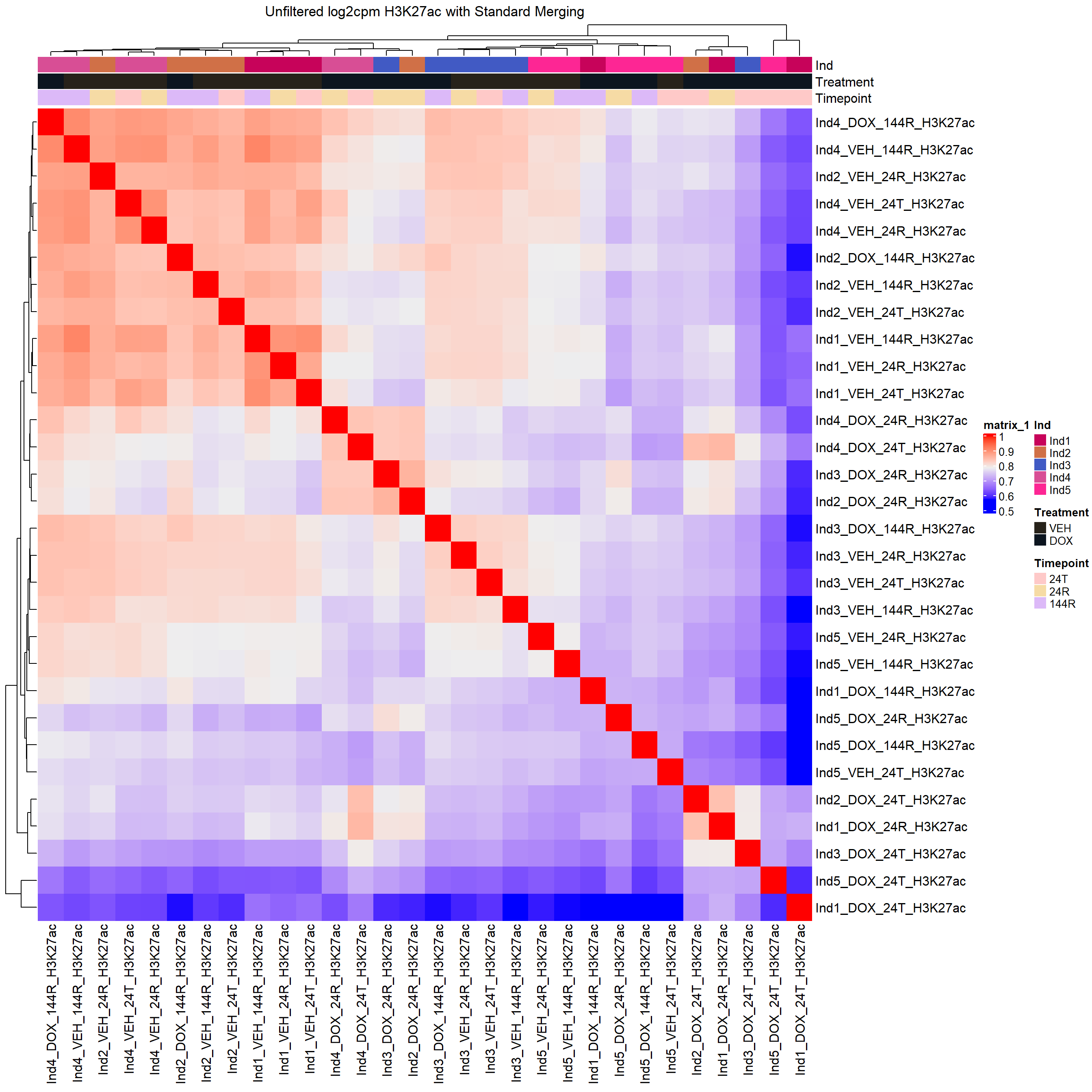

Version	Author	Date
1160ce2	infurnoheat	2025-07-24
66c1fa7	infurnoheat	2025-07-24
389b998	infurnoheat	2025-07-23
d927f5c	infurnoheat	2025-07-23

annomat <- data.frame(sample=colnames(H3K27ac_cluster_cor)) %>% 
  separate_wider_delim(sample,delim="_",names=c("Ind","Treatment","Timepoint",NA),cols_remove = FALSE) %>% 
  mutate(Treatment=factor(Treatment, levels = c("VEH","5FU","DOX")),
         Timepoint=factor(Timepoint, levels =c("24T","24R","144R"))) %>% 
  column_to_rownames("sample")
heatmap_first <- ComplexHeatmap::HeatmapAnnotation(df = annomat)

Heatmap(H3K27ac_cluster_cor, 
        top_annotation = heatmap_first,
        column_title="Unfiltered log2cpm H3K27ac with Cluster Merging")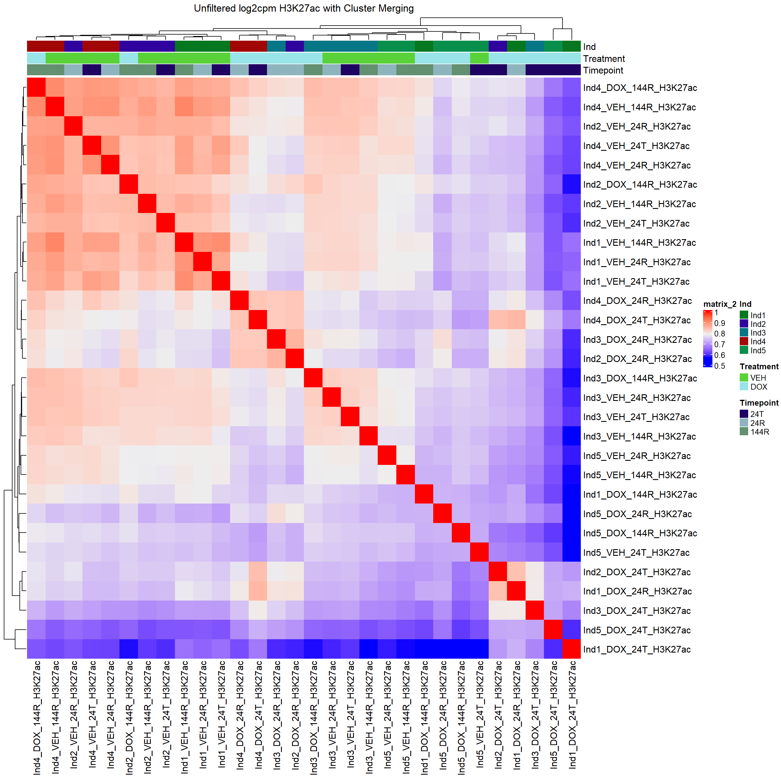

Version	Author	Date
1160ce2	infurnoheat	2025-07-24
66c1fa7	infurnoheat	2025-07-24
389b998	infurnoheat	2025-07-23
d927f5c	infurnoheat	2025-07-23

annomat <- data.frame(sample=colnames(H3K27ac_iter_cor)) %>% 
  separate_wider_delim(sample,delim="_",names=c("Ind","Treatment","Timepoint",NA),cols_remove = FALSE) %>% 
  mutate(Treatment=factor(Treatment, levels = c("VEH","5FU","DOX")),
         Timepoint=factor(Timepoint, levels =c("24T","24R","144R"))) %>% 
  column_to_rownames("sample")
heatmap_first <- ComplexHeatmap::HeatmapAnnotation(df = annomat)

Heatmap(H3K27ac_iter_cor, 
        top_annotation = heatmap_first,
        column_title="Unfiltered log2cpm H3K27ac with Iterative Merging")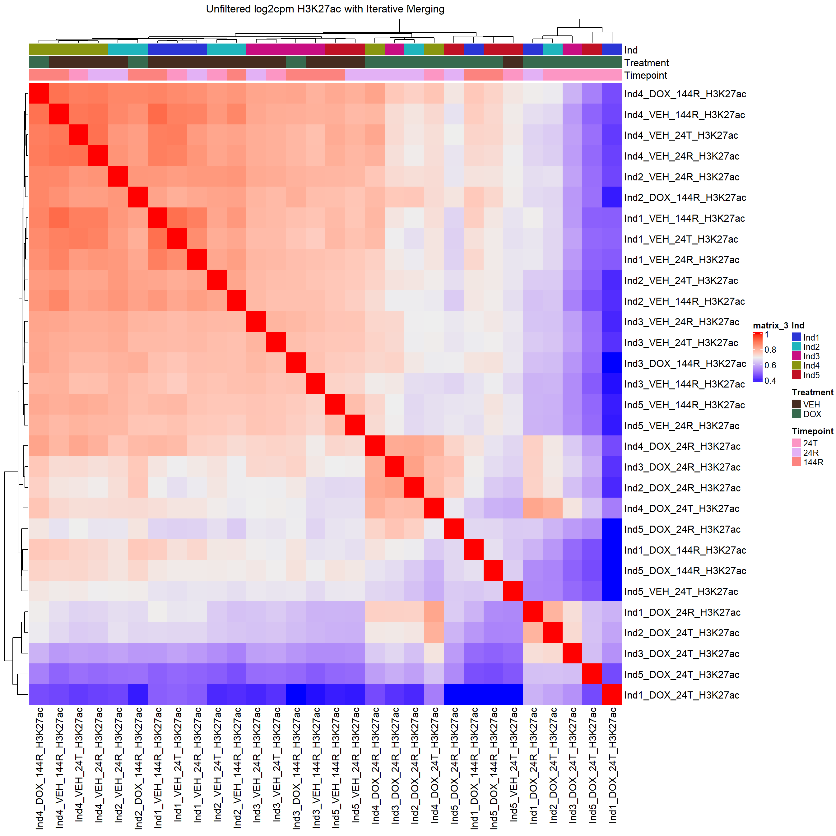

Version	Author	Date
1160ce2	infurnoheat	2025-07-24
66c1fa7	infurnoheat	2025-07-24
389b998	infurnoheat	2025-07-23
d927f5c	infurnoheat	2025-07-23

H3K27me3 Count Analysis

H3K36me3 Count Analysis

H3K9me3 Count Analysis

Fragment Analysis

all_peak %>%
  mutate(Fragments=Fragments/1000000) %>% 
  ggplot(., aes(x=interaction(Individual,Treatment,Timepoint), y=Fragments, fill=Treatment, group = Treatment))+
  geom_col()+
  geom_hline(yintercept =5)+
  geom_text(aes(y = 0,label = Sample), vjust = 0.2, size = 3, angle = 90)+
  theme_classic()+
  facet_wrap(~Histone_Mark)+
  ggtitle("Fragment count by histone and sample")+
  ylab("Count of Fragments * 10^6")+
  xlab("Samples")+
  theme(axis.text.x=element_text(vjust = .2,angle=90))+
  scale_y_continuous( expand = expansion(mult = c(0, .1)))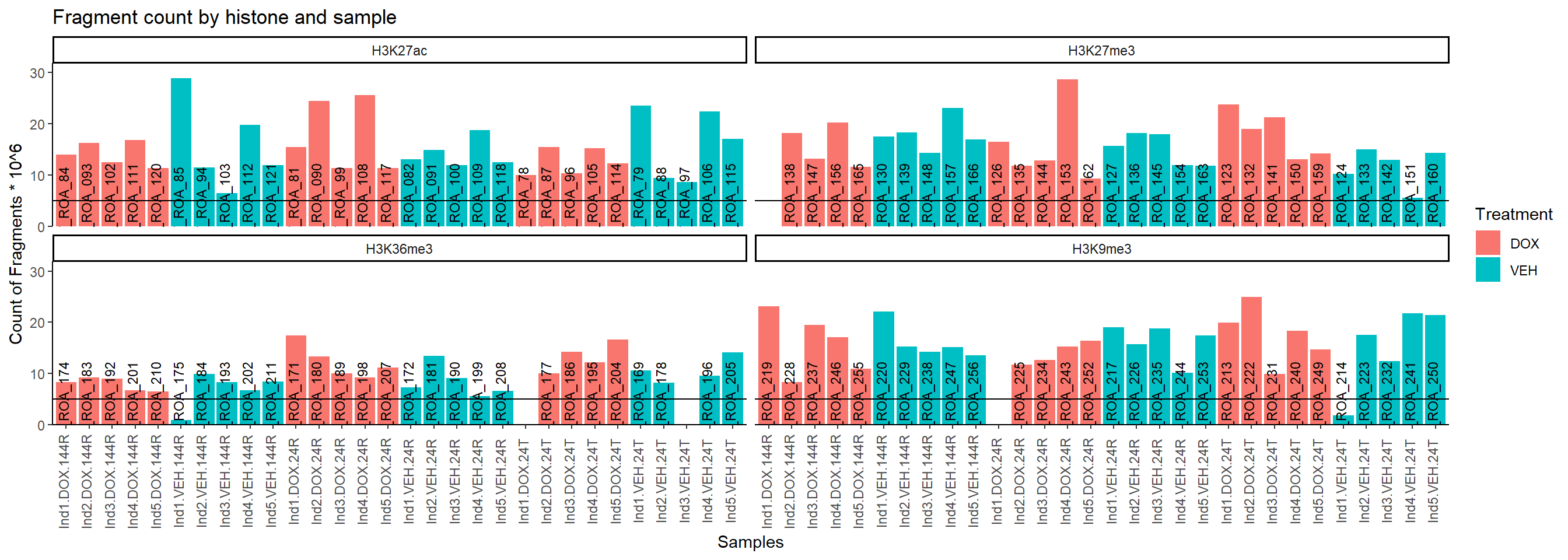

Version	Author	Date
389b998	infurnoheat	2025-07-23

all_peak %>%
  mutate(FRiP=FRiP * 100) %>% 
  ggplot(., aes(x=interaction(Individual,Treatment,Timepoint), y=FRiP, fill=Treatment, group = Treatment))+
  geom_col()+
  geom_hline(yintercept =5)+
  geom_text(aes(y = 0,label = Sample), vjust = 0.2, size = 3, angle = 90)+
  theme_classic()+
  facet_wrap(~Histone_Mark)+
  ggtitle("Fragment count by histone and sample")+
  ylab("Count of Fragments * 10^6")+
  xlab("Samples")+
  theme(axis.text.x=element_text(vjust = .2,angle=90))+
  scale_y_continuous( expand = expansion(mult = c(0, .1)))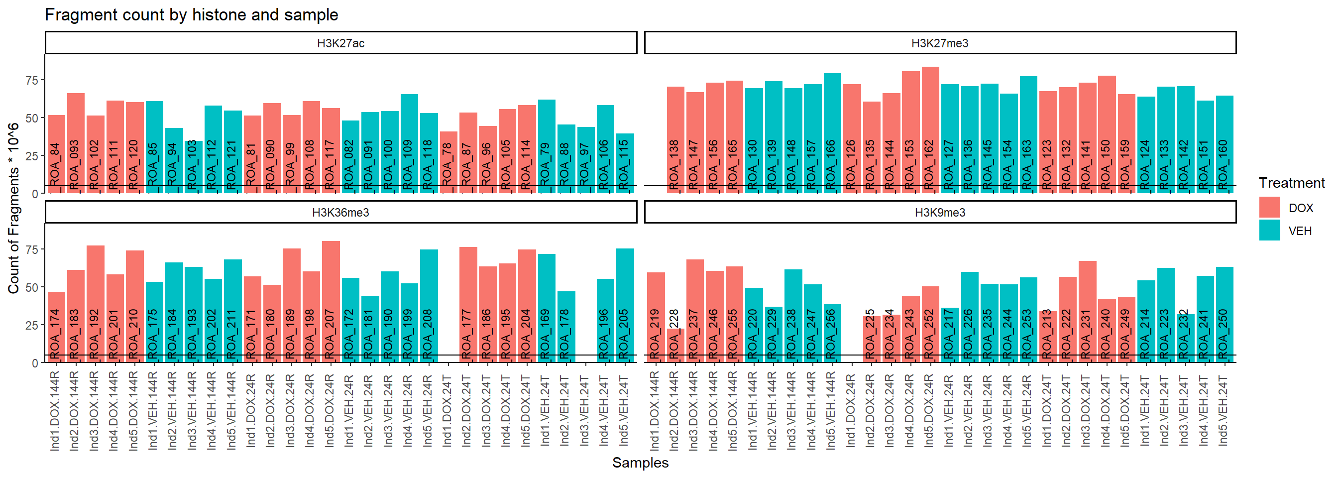

Version	Author	Date
389b998	infurnoheat	2025-07-23

sessionInfo()

R version 4.5.1 (2025-06-13 ucrt)
Platform: x86_64-w64-mingw32/x64
Running under: Windows 11 x64 (build 26100)

Matrix products: default
  LAPACK version 3.12.1

locale:
[1] LC_COLLATE=English_United States.utf8 
[2] LC_CTYPE=English_United States.utf8   
[3] LC_MONETARY=English_United States.utf8
[4] LC_NUMERIC=C                          
[5] LC_TIME=English_United States.utf8    

time zone: America/Chicago
tzcode source: internal

attached base packages:
[1] stats4    grid      stats     graphics  grDevices utils     datasets 
[8] methods   base     

other attached packages:
 [1] Rsubread_2.22.1             gcplyr_1.11.0              
 [3] ggpmisc_0.6.2               ggpp_0.5.9                 
 [5] corrplot_0.95               ggpubr_0.6.1               
 [7] DESeq2_1.48.1               SummarizedExperiment_1.38.1
 [9] Biobase_2.68.0              MatrixGenerics_1.20.0      
[11] matrixStats_1.5.0           chromVAR_1.30.1            
[13] GenomicRanges_1.60.0        GenomeInfoDb_1.44.0        
[15] IRanges_2.42.0              S4Vectors_0.46.0           
[17] BiocGenerics_0.54.0         generics_0.1.4             
[19] genomation_1.40.1           kableExtra_1.4.0           
[21] DT_0.33                     viridis_0.6.5              
[23] viridisLite_0.4.2           data.table_1.17.8          
[25] ComplexHeatmap_2.24.1       edgeR_4.6.3                
[27] limma_3.64.1                lubridate_1.9.4            
[29] forcats_1.0.0               stringr_1.5.1              
[31] dplyr_1.1.4                 purrr_1.1.0                
[33] readr_2.1.5                 tidyr_1.3.1                
[35] tibble_3.3.0                ggplot2_3.5.2              
[37] tidyverse_2.0.0             workflowr_1.7.1            

loaded via a namespace (and not attached):
  [1] splines_4.5.1               later_1.4.2                
  [3] BiocIO_1.18.0               bitops_1.0-9               
  [5] XML_3.99-0.18               DirichletMultinomial_1.50.0
  [7] lifecycle_1.0.4             pwalign_1.4.0              
  [9] rstatix_0.7.2               doParallel_1.0.17          
 [11] rprojroot_2.1.0             vroom_1.6.5                
 [13] MASS_7.3-65                 processx_3.8.6             
 [15] lattice_0.22-7              backports_1.5.0            
 [17] magrittr_2.0.3              plotly_4.11.0              
 [19] sass_0.4.10                 rmarkdown_2.29             
 [21] jquerylib_0.1.4             yaml_2.3.10                
 [23] plotrix_3.8-4               httpuv_1.6.16              
 [25] DBI_1.2.3                   RColorBrewer_1.1-3         
 [27] abind_1.4-8                 RCurl_1.98-1.17            
 [29] git2r_0.36.2                circlize_0.4.16            
 [31] GenomeInfoDbData_1.2.14     seqLogo_1.74.0             
 [33] MatrixModels_0.5-4          svglite_2.2.1              
 [35] codetools_0.2-20            DelayedArray_0.34.1        
 [37] xml2_1.3.8                  tidyselect_1.2.1           
 [39] shape_1.4.6.1               UCSC.utils_1.4.0           
 [41] farver_2.1.2                GenomicAlignments_1.44.0   
 [43] jsonlite_2.0.0              GetoptLong_1.0.5           
 [45] Formula_1.2-5               survival_3.8-3             
 [47] iterators_1.0.14            systemfonts_1.2.3          
 [49] foreach_1.5.2               tools_4.5.1                
 [51] TFMPvalue_0.0.9             Rcpp_1.0.14                
 [53] glue_1.8.0                  gridExtra_2.3              
 [55] SparseArray_1.8.0           xfun_0.52                  
 [57] withr_3.0.2                 fastmap_1.2.0              
 [59] SparseM_1.84-2              callr_3.7.6                
 [61] caTools_1.18.3              digest_0.6.37              
 [63] timechange_0.3.0            R6_2.6.1                   
 [65] mime_0.13                   seqPattern_1.40.0          
 [67] textshaping_1.0.1           colorspace_2.1-1           
 [69] gtools_3.9.5                RSQLite_2.4.1              
 [71] rtracklayer_1.68.0          httr_1.4.7                 
 [73] htmlwidgets_1.6.4           S4Arrays_1.8.1             
 [75] TFBSTools_1.46.0            whisker_0.4.1              
 [77] pkgconfig_2.0.3             gtable_0.3.6               
 [79] blob_1.2.4                  impute_1.82.0              
 [81] XVector_0.48.0              htmltools_0.5.8.1          
 [83] carData_3.0-5               clue_0.3-66                
 [85] scales_1.4.0                png_0.1-8                  
 [87] knitr_1.50                  rstudioapi_0.17.1          
 [89] tzdb_0.5.0                  reshape2_1.4.4             
 [91] rjson_0.2.23                curl_6.4.0                 
 [93] cachem_1.1.0                GlobalOptions_0.1.2        
 [95] KernSmooth_2.23-26          parallel_4.5.1             
 [97] miniUI_0.1.2                restfulr_0.0.16            
 [99] pillar_1.11.0               vctrs_0.6.5                
[101] promises_1.3.3              car_3.1-3                  
[103] xtable_1.8-4                cluster_2.1.8.1            
[105] evaluate_1.0.4              cli_3.6.5                  
[107] locfit_1.5-9.12             compiler_4.5.1             
[109] Rsamtools_2.24.0            rlang_1.1.6                
[111] crayon_1.5.3                ggsignif_0.6.4             
[113] labeling_0.4.3              ps_1.9.1                   
[115] getPass_0.2-4               plyr_1.8.9                 
[117] fs_1.6.6                    stringi_1.8.7              
[119] gridBase_0.4-7              BiocParallel_1.42.1        
[121] Biostrings_2.76.0           lazyeval_0.2.2             
[123] quantreg_6.1                Matrix_1.7-3               
[125] BSgenome_1.76.0             hms_1.1.3                  
[127] bit64_4.6.0-1               statmod_1.5.0              
[129] shiny_1.11.1                broom_1.0.8                
[131] memoise_2.0.1               bslib_0.9.0                
[133] bit_4.6.0                   polynom_1.4-1

Peak Analysis

Steven Yu

2025-07-14

Peak Anaylsis

Loading Packages

Data Initialization

Functions

Peak Calling for Q=0.01 and Broad=0.1 with No Lambda

Data Initialization

Peak Visualization

Peak Calling for Q=0.01 and Broad=0.1 with Lambda

Data Initialization

Peak Visualization

Peak Calling for Q=0.01 and Broad=0.5 with No Lambda

Data Initialization

Peak Visualization

Peak Calling for Q=0.01 and Broad=0.5 with Lambda

Data Initialization

Peak Visualization

Peak Calling for Q=0.005 and Broad=0.01 with No Lambda

Data Initialization

Peak Visualization

Peak Calling for Q=0.005 and Broad=0.01 with Lambda

Data Initialization

Peak Visualization

Picard with Broad Peaks

Picard with Broad as Narrow Peaks

Picard with Broad as Stringent Narrow Peaks

Tagging Questionable Libraries by FRiP

Peak Widths

Peak Width Function

Broad Visualization

Broad as Narrow Visualization

Broad as Narrow Stringent Visualization

Feature Counts

H3K27ac Count Analysis

H3K27me3 Count Analysis

H3K36me3 Count Analysis

H3K9me3 Count Analysis

Fragment Analysis