Dates and times with Lubridate
I2DS Tools for Data Science Workshop
Introduction
In this workshop, we’ll introduce you to the Lubridate package, a useful tool to work with dates and times in R.
Objectives of the session:
Understand the core components of lubridate.
To learn how to handle date and time data effectively.
To apply this knowledge to real-world data analysis and visualization tasks.
What is lubridate? ⏲
Lubridate simplifies date and time data manipulation in R.
It provides an intuitive and consistent interface for creating, parsing, and performing operations on date-time objects.
This package offers a set of standardized functions for analyze dates, performing arithmetic with date-time data, and extracting specific components of date and time formats (e.g., year, month, day).
Load the package lubridate 🔛
The easiest way to get lubridate is to install the whole tidyverse:
Alternatively, install just lubridate:
Or the the development version from GitHub:
Creating date/times 📆
There are three types of date/time data that refer to an instant in time:
- A date. Tibbles print this as date.
- A time within a day. Tibbles print this as time.
- A date-time is a date plus a time: it uniquely identifies an instant in time (typically to the nearest second). Tibbles print this as dttm.
To get the current date or date-time you can use today() or now():
## [1] "2023-10-27"## [1] "2023-10-27 16:45:16 CEST"The phrase “CEST” in the output represents the time-zone, this stands for Central European Summer Time. By default it should be “UTC”.
*You can use the ‘OlsonNames()’ function to locate the continent or city you wish to use.
You can determine either the ‘UTC’ time or the current time in another country.
## [1] "2023-10-27 14:45:16 UTC"## [1] "2023-10-27 21:45:16 +07"Parsing dates and times: 🔍
Using lubridate, we have the capability to parse dates by employing a combination of the letters ‘d’ (representing day), ‘m’ (representing month), and ‘y’ (representing year). We simply match the letters to the pattern of the date we are trying to parse.
For example, let’s consider the date May 31, 2023. We can represent it either numerically without spaces or as a string using either ‘-’ or ‘/’.”
#Let's see how it will appear when we begin with the year.
ymd(20230531)

#Let's see how it will appear when we begin with the month.
mdy("05-31-2023")

#Let's see how it will appear when we begin with the day.
dmy("31/05/2023")

#Also, we can write our date like this
mdy("May 31st, 2023")
dmy("31 of May 2023")
ymd() and friends create dates. To create a date-time, add an underscore and one or more of “h”, “m”, and “s” to the name of the parsing function:
## [1] "20H 11M 59S"## [1] "2023-05-31 20:11:59 UTC"## [1] "2023-05-31 20:11:00 UTC"## [1] "2023-05-31 20:00:00 UTC"Components: 🔮
If the date-time variable is successfully parsed as a date-time class then we can begin extracting components.
Can you extract date, year, month, hour, minutes and seconds from the date May 31, 2023?
## [1] "2023-05-31"## [1] 2023## [1] 5## [1] 31## [1] 20## [1] 11## [1] 59## [1] 22## [1] 2## [1] 1TED Talks 🔉
These datasets contain information about all audio-video recordings of TED Talks uploaded to the official TED.com website until September 21st, 2017.
Features Available:
- name: The official name of the TED Talk. Includes the title and the speaker.
- title: The title of the talk
- description: A blurb of what the talk is about.
- main_speaker: The first named speaker of the talk.
- speaker_occupation: The occupation of the main speaker.
- num_speaker: The number of speakers in the talk.
- duration: The duration of the talk in seconds.
- event: The TED/TEDx event where the talk took place.
- film_date: The Unix timestamp of the filming.
- published_date: The Unix timestamp for the publication of the talk on TED.com
- comments: The number of first level comments made on the talk.
- tags: The themes associated with the talk.
- languages: The number of languages in which the talk is available.
- ratings: A stringified dictionary of the various ratings given to the talk (inspiring, fascinating, jaw dropping, etc.)
- related_talks: A list of dictionaries of recommended talks to watch next.
- url: The URL of the talk.
- views: The number of views on the talk.
More about dataset:https://www.kaggle.com/datasets/rounakbanik/ted-talks/data
##  [1] "comments"           "description"        "duration"
##  [4] "event"              "film_date"          "languages"
##  [7] "main_speaker"       "name"               "num_speaker"
## [10] "published_date"     "ratings"            "related_talks"
## [13] "speaker_occupation" "tags"               "title"
## [16] "url"                "views"
There are three columns containing dates and times: “film_date”, “published_date”, “duration”. Let’s see how they look like:
The date “1140825600” (or “1151367060”, “1164”) appears to be a timestamp. In many programming languages and systems, timestamps are typically measured in seconds or milliseconds since a reference point in time, often referred to as the “Unix epoch.”
We can convert this Unix timestamp to a date using the “as_datetime”, “as.duration” function:
ted$published_date <- as_datetime(ted$published_date)
ted$film_date <- as_datetime(ted$film_date)
ted$duration <- as.duration(ted$duration)
ted_selected <- ted |>
  select(film_date, published_date, duration) |>
  head()
ted_selected
Does the duration of the TED talk video affect the number of views?
#Most views
ted_compare_v <- ted |>
  arrange(desc(views)) |>
  head(5) |>
  select(duration, views)
ted_compare_v
#Least views
ted_compare_views <- ted |>
arrange(views) |>
head(5) |>
select(duration, views)
ted_compare_viewsDoes the hour when the video was posted affect the views?
Extract hour from the published_date and compare with views:
#Most views
ted_compare_h <- ted |>
  mutate(hour_publ = hour(published_date)) |>
  arrange(desc(views)) |>
  head(5) |>
  select(hour_publ, views)
ted_compare_h
#Least views
ted_compare_hour <- ted |>
mutate(hour_publ = hour(published_date)) |>
arrange(views) |>
head(5) |>
select(hour_publ, views)
ted_compare_hourDoes the year affect the number of comments?
Extract year from the published_date and compare with comments:
#Most comments
ted_compare_y <- ted |>
  mutate(year_publ = year(published_date)) |>
  arrange(desc(comments)) |>
  head(5) |>
  select(year_publ, comments)
ted_compare_y
#Least comments
ted_compare_year <- ted |>
mutate(year_publ = year(published_date)) |>
arrange(comments) |>
head(5) |>
select(year_publ, comments)
ted_compare_yearggplot(data = ted, aes(x = published_date, y = comments)) +
geom_line() +
labs(x = "Date of Publication", y = "Comments") +
ggtitle("Comments vs. Date of Publication")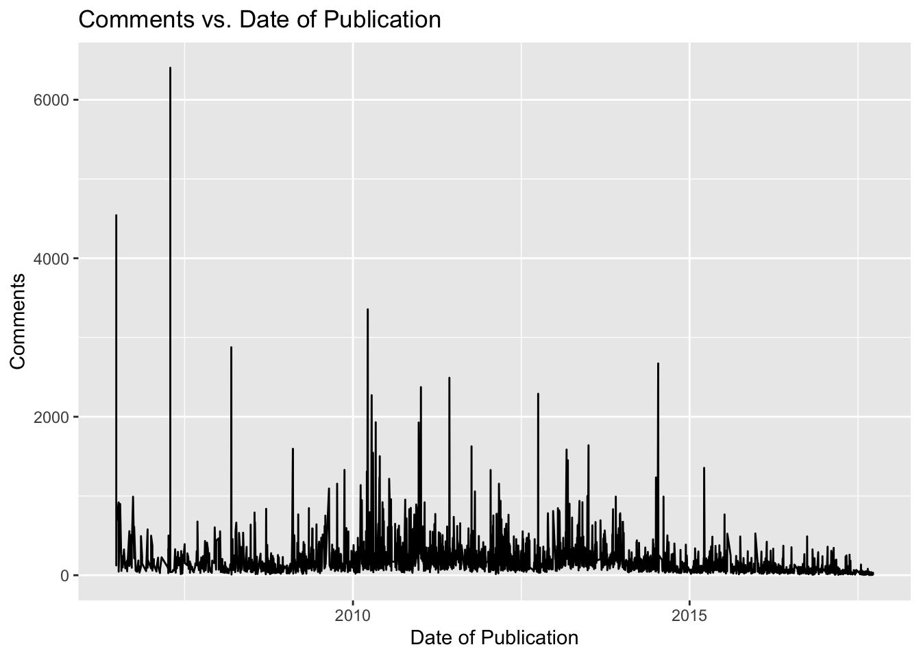
A work by Monserrat López and Anzhelika Belozerova. Template of Lisa Oswald & Tom Arend.
I2DS Tools for Data Science Workshop by Simon Munzert