In [4]:
%%capture --no-display
%%R -w 800 -h 800 -u px
p1 <- plotEmbedding(ArchRProj = proj.orig, colorBy = "cellColData", name = "Clusters", embedding = "UMAP") + ggtitle("Human lung snATAC-seq(74930 nuclei)")
p1 + theme_ArchR(baseSize = 12)

Background
GWAS findings on adult Asthma show many loci harbon genes related to immune functions. For instance...Researchers have shown peripheral blood immune cells contribute to the heritability of Asthma but at a limited level.
Specific problem
Can we leverage single-cell ATAC-seq data that characterize chromatin openness in relevant cell types to explain broader heriability of Asthma?
Objectives
The goal for this analysis is to identify tissue-resident T cells in the snATAC-seq data of lung tissues, which would be utilized to improve annotations for Asthma's risk variants.
%load_ext rpy2.ipython
/home/jinggu/scratch-midway2/tools/miniconda3/lib/python3.7/site-packages/rpy2/robjects/pandas2ri.py:14: FutureWarning: pandas.core.index is deprecated and will be removed in a future version.  The public classes are available in the top-level namespace.
  from pandas.core.index import Index as PandasIndex
%%capture
%%R
library("ArchR")
library(Matrix)
library("Seurat")
library(repr)
library("dplyr")
#Load ArchR object
proj<-loadArchRProject("~/cluster/projects/lung_subset/")
proj.orig<-loadArchRProject("lung_snATAC/")
%%capture --no-display
%%R -w 800 -h 800 -u px
p1 <- plotEmbedding(ArchRProj = proj.orig, colorBy = "cellColData", name = "Clusters", embedding = "UMAP") + ggtitle("Human lung snATAC-seq(74930 nuclei)")
p1 + theme_ArchR(baseSize = 12)
addGeneScoreMatrix()
For a given gene, ArchR utilized the local accessibility of the gene region (promoter and gene body) and distal accessibility of the gene window that do not cross over other gene regions to predict gene expression values. ArchR partition our genome into 500bp overlapping tiles. For each tile, ArchR scales gene size weights and together with distance weights are then multiplied by the number of Tn5 insertions. A final gene score is generated by summing up the scores across all tiles within the gene window.
%%capture --no-display
%%R -w 1000 -h 1000 -u px
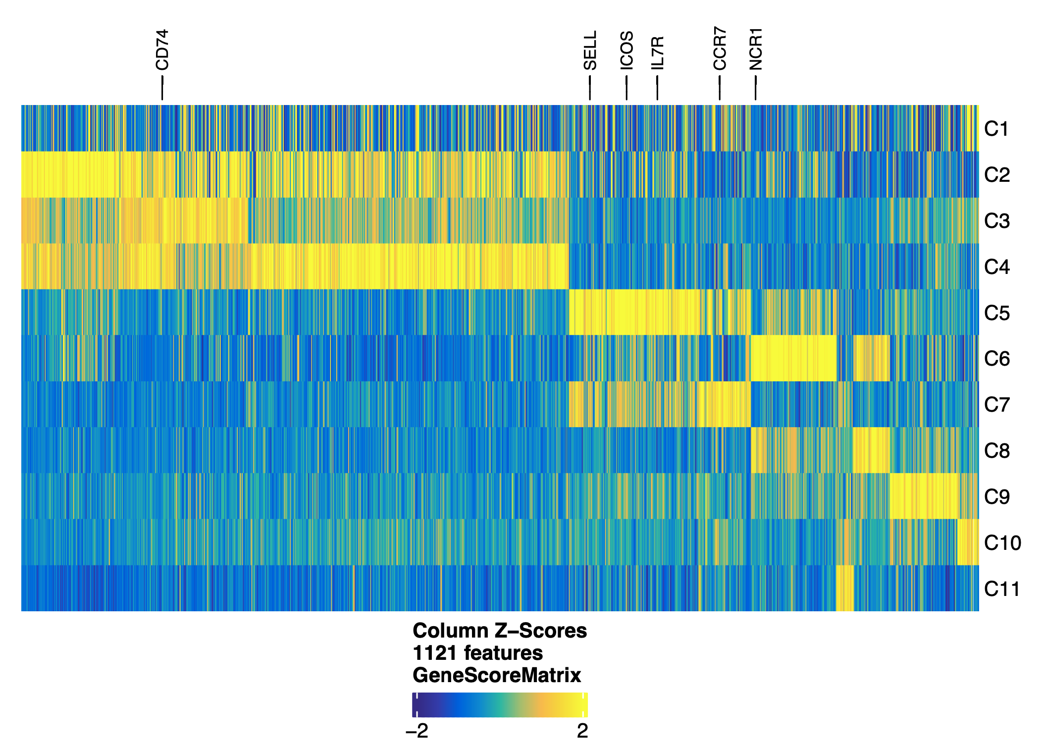
load(file="/home/jinggu/cluster/projects/lung_snATAC/Objects/markersGS.Rdata")
markerList <- getMarkers(markersGS, cutOff = "FDR <= 0.01 & Log2FC >= 1.25")
markerGenes <- c(
'TEKT4','KRT5','SCGB3A2',
'ASCL1','SFTPC','WNT7A',
'PDGFRB','MYOCD','WNT2',
'PROX1','CA4','VWF',
'ICOS','NCR1','MS4A1',
'GATA1','CD68','TCF7',
'CD8A','CD4','CD74','PRF1',
'CCR7', 'ITGAE','CD69'
)
#make a heatmap labeled with marker genes
heatmapGS <- markerHeatmap(
seMarker = markersGS,
cutOff = "FDR <= 0.01 & Log2FC >= 1.25",
labelMarkers = markerGenes,
transpose = TRUE
)
ComplexHeatmap::draw(heatmapGS, heatmap_legend_side = "bot", annotation_legend_side = "bot")

%%capture --no-display
%%R -w 800 -h 800 -u px
remapClust<-c("C1"="Endothelial cells","C2"="Endothelial cells","C3"="Endothelial cells",
              "C4"="Epithelial cells", "C5"="Epithelial cells", "C6"="Epithelial cells", "C7"="Epithelial cells",
              "C8"="Epithelial cells", "C9"="Epithelial cells",
              "C10"="Mesenchymal cells", "C11"="Mesenchymal cells", "C12"="Mesenchymal cells",
              "C13"="Mesenchymal cells","C14"="Mesenchymal cells",
              "C15"="Epithelial cells", "C16"="Epithelial cells",
              "C17"= "Erythrocytes","C18"= "Erythrocytes",
              "C22"= "B cells", "C19"="T/NK cells", "C20"="T/NK cells",
              "C21"="T/NK cells","C23"="T/NK cells", "C24"="T/NK cells","C25"="T/NK cells")

labelNew2 <- mapLabels(proj.orig$Clusters, oldLabels = names(remapClust), newLabels = remapClust)
proj.orig$Clusters_GS<-labelNew2
p1 <- plotEmbedding(ArchRProj = proj.orig, colorBy = "cellColData", name = "Clusters_GS", size=0.2, baseSize=15,
                    embedding = "UMAP") + ggtitle("Human lung snATAC-seq(74930 nuclei)")
%%capture
%%R
#predict gene scores for marker genes
markerGenes  <- c(
    'NCR1','CD8A','CD4','CD74',
    'CCR7', 'ITGAE','CD69',
    'IL7R', 'ICOS'
  )
#proj.orig <- addImputeWeights(proj.orig)
#make plots for marker genes
p <- plotEmbedding(
    ArchRProj = proj.orig,
    colorBy = "GeneScoreMatrix",
    name = markerGenes,
    embedding = "UMAP",
    imputeWeights = getImputeWeights(proj.orig)
)
#Rearrange for grid plotting
p2 <- lapply(p, function(x){
    x + guides(color = FALSE, fill = FALSE) +
    theme_ArchR(baseSize = 12) +
    theme(plot.margin = unit(c(0, 0, 0, 0), "cm")) +
    theme(
        axis.text.x=element_blank(),
        axis.ticks.x=element_blank(),
        axis.text.y=element_blank(),
        axis.ticks.y=element_blank()
    )
})
%%capture --no-display
%%R -w 800 -h 800 -u px
do.call(cowplot::plot_grid, c(list(ncol = 3),p2))

Align cells from scATAC-seq data to those from scRNA-seq data by comparing the scATAC-seq gene score matrix with scRNA-seq gene expression matrix
%%R -w 800 -h 800 -u px
lung.rna<-readRDS("~/cluster/projects/lung_others/lung_scRNA/lung_Wang2020.rds")
DimPlot(lung.rna, reduction = "umap", label = TRUE, pt.size = 0.5) + NoLegend() +
ggtitle("Human lung snRNA-Seq (46500 nuclei)")

Procedures:
%%R
tcell.rna<-readRDS("~/cluster/projects/lung_others/lung_scRNA/lung_Tcell_subclustering_Wang2020.rds")
DimPlot(tcell.rna, reduction = "umap", label = TRUE, pt.size = 0.5) + NoLegend() + ggtitle("Human lung snRNA-Seq T cells (3209 nuclei)")

Y-axis: Top 10 differentially expressed genes for each subcluster
%%R -w 800 -h 800 -u px
cluster.markers<-read.table("~/cluster/projects//lung_others//lung_scRNA//t_cell_subclusters_DEG.txt", header = T)
cluster.markers %>%
    group_by(cluster) %>%
    top_n(n = 10, wt = avg_log2FC) -> top10
DoHeatmap(tcell.rna, features = top10$gene) + NoLegend()

%%R
cluster1.markers<-FindMarkers(tcell.rna, ident.1 = c(0,1), ident.2 = seq(2,6), min.pct = 0.1)
cluster1.markers[which(rownames(cluster1.markers)=="CD69"),]
           p_val avg_log2FC pct.1 pct.2    p_val_adj
CD69 5.81979e-09 -0.3943621 0.282  0.37 0.0001546784
%%R
new.cluster.ids<-c("0"="unknown", "1"="Non-TR cells", "2"="TR cells", "3"="TR cells",
                   "4"="TR cells", "5"="TR cells", "6"="TR cells")

tcell.rna<-RenameIdents(tcell.rna, new.cluster.ids)
DimPlot(tcell.rna, reduction = "umap", label = TRUE, pt.size = 0.5) + NoLegend()

%%R -w 800 -h 400 -u px
markerGenes  <- c(
    'CCR7', 'ITGAE','CD69')
VlnPlot(tcell.rna, features = markerGenes, slot = "counts", log = TRUE)

Procedures:
%%capture --no-display
%%R -w 800 -h 800 -u px
p2 <- plotEmbedding(ArchRProj = proj, colorBy = "cellColData", name = "Clusters", embedding = "UMAP", title="Sub-clustering of T cell/NK cells")
p2+ theme_ArchR(baseSize = 12)

%%capture
%%R
#predict gene scores for marker genes
markerGenes  <- c(
    'NCR1','CD8A','CD4','CD74',
    'CCR7', 'ITGAE','CD69',
    'IL7R', 'ICOS'
  )
proj<- addImputeWeights(proj)
#make plots for marker genes
p <- plotEmbedding(
    ArchRProj = proj,
    colorBy = "GeneScoreMatrix",
    name = markerGenes,
    embedding = "UMAP",
    imputeWeights = getImputeWeights(proj)
)
#Rearrange for grid plotting
p2 <- lapply(p, function(x){
    x + guides(color = FALSE, fill = FALSE) +
    theme_ArchR(baseSize = 6.5) +
    theme(plot.margin = unit(c(0, 0, 0, 0), "cm")) +
    theme(
        axis.text.x=element_blank(),
        axis.ticks.x=element_blank(),
        axis.text.y=element_blank(),
        axis.ticks.y=element_blank()
    )
})
%%capture --no-display
%%R -w 800 -h 800 -u px
do.call(cowplot::plot_grid, c(list(ncol = 3),p2))

%%capture
%%R
tcell.rna$cell_types<-tcell.rna@active.ident
head(tcell.rna)
projInteg <- addGeneIntegrationMatrix(
    ArchRProj = proj,
    useMatrix = "GeneScoreMatrix",
    matrixName = "GeneIntegrationMatrix",
    reducedDims = "IterativeLSI",
    seRNA = tcell.rna,
    addToArrow = FALSE,
    groupRNA = "cell_types",
    nameCell = "predictedCell_Un",
    nameGroup = "predictedGroup_Un",
    nameScore = "predictedScore_Un"
)
%%R
#Unconstrained integration
cM <- as.matrix(confusionMatrix(projInteg$Clusters, projInteg$predictedGroup_Un))
preClust <- colnames(cM)[apply(cM, 1 , which.max)]
cbind(preClust, rownames(cM)) #Assignments
      preClust
 [1,] "unknown"      "C10"
 [2,] "unknown"      "C3"
 [3,] "TR cells"     "C8"
 [4,] "Non-TR cells" "C7"
 [5,] "TR cells"     "C9"
 [6,] "TR cells"     "C11"
 [7,] "Non-TR cells" "C5"
 [8,] "unknown"      "C4"
 [9,] "unknown"      "C2"
[10,] "TR cells"     "C6"
[11,] "unknown"      "C1"
%%R
cM
    unknown TR cells Non-TR cells
C10     352      249            5
C3      322      320            0
C8      291      803            0
C7       43       99          671
C9      267     1132           20
C11      20      796            2
C5       64      164          322
C4      610      113            1
C2      106       71            1
C6       50      237            0
C1       46        1            0
%%R
#Constrained Integration
clustTNK <- rownames(cM)[grep("TR cells", preClust)]
clustTNK
clustNonTNK <- paste0("C", 1:10)[!(paste0("C", 1:10) %in% clustTNK)]
clustNonTNK
rnaTNK <- rownames(tcell.rna@meta.data[tcell.rna$cell_types=="TR cells",])
rnaNonTNK <- rownames(tcell.rna@meta.data[tcell.rna$cell_types!="TR cells",])
[1] "C1" "C2" "C3" "C4" "C10"
%%R
groupList <- SimpleList(
    TNK = SimpleList(
        ATAC = projInteg$cellNames[projInteg$Clusters %in% clustTNK],
        RNA = rnaTNK
    ),
    NonTNK = SimpleList(
        ATAC = projInteg$cellNames[projInteg$Clusters %in% clustNonTNK],
        RNA = rnaNonTNK
    )
)

projInteg <- addGeneIntegrationMatrix(
    ArchRProj = projInteg,
    useMatrix = "GeneScoreMatrix",
    matrixName = "GeneIntegrationMatrix",
    reducedDims = "IterativeLSI",
    seRNA = tcell.rna,
    addToArrow = FALSE,
    groupList = groupList,
    groupRNA = "cell_types",
    nameCell = "predictedCell_Co",
    nameGroup = "predictedGroup_Co",
    nameScore = "predictedScore_Co"
)
pal <- paletteDiscrete(values = unique(tcell.rna$cell_types))
p1 <- plotEmbedding(
    projInteg,
    colorBy = "cellColData",
    name = "predictedGroup_Un",
    pal = pal
)
p2 <- plotEmbedding(
    projInteg,
    colorBy = "cellColData",
    name = "predictedGroup_Co",
    pal = pal
)
%%R
p1

%%R
p2

%%R
projPeakcalling<-addGroupCoverages(
    ArchRProj = projInteg,
    groupBy = "predictedGroup_Un",
)
projPeakcalling<-addReproduciblePeakSet(
    ArchRProj = projPeakcalling,
    groupBy = "predictedGroup_Un",
    pathToMacs2="/scratch/midway2/jinggu/env/sc-atac/bin/macs2"
)

output<-getPeakSet(projPeakcalling)
save(output, file="~/cluster/projects/archR/tissueRes_T_cells_Wang2020.Rdata")
saveArchRProject(ArchRProj = projPeakcalling, outputDirectory = "/home/jinggu/cluster/projects/archR/tissueRes_tcells", load = FALSE)
%%R -w 800 -h 800 -u px
library(ggplot2)
source("~/projects/funcFinemapping/code/make_plots.R")
tbl<-data.frame()
for(trait in c("allergy", "asthma_adult", "asthma_child")){
  df<-read.table(sprintf("~/projects/funcFinemapping/output/AAD/%s/Wang2020_indiv.est", trait), header=F)
  colnames(df)<-c("raw_term", "estimate", "low", "high")
  df["term"]<-unlist(lapply(df$raw_term, function(i){strsplit(i, "[.]")[[1]][1]}))
  tbl<-data.frame(rbind(tbl, cbind(df, trait)))
}

snp_enrichment_plot(tbl, trait="", y.order = c()) + facet_grid(. ~ trait)

Note: Tissue-resident T cells show significant enrichment for adult-onset asthma but not for child-onset asthma. The enrichment estimates for tissue-resident T cells are lower than pseudobulk T cells.