This reproducible R Markdown
analysis was created with workflowr (version
1.7.0). The Checks tab describes the reproducibility checks
that were applied when the results were created. The Past
versions tab lists the development history.
The R Markdown file has unstaged changes. To know which version of
the R Markdown file created these results, you’ll want to first commit
it to the Git repo. If you’re still working on the analysis, you can
ignore this warning. When you’re finished, you can run
wflow_publish to commit the R Markdown file and build the
HTML.
Great job! The global environment was empty. Objects defined in the
global environment can affect the analysis in your R Markdown file in
unknown ways. For reproduciblity it’s best to always run the code in an
empty environment.
The command set.seed(12345) was run prior to running the
code in the R Markdown file. Setting a seed ensures that any results
that rely on randomness, e.g. subsampling or permutations, are
reproducible.
Great! You are using Git for version control. Tracking code development
and connecting the code version to the results is critical for
reproducibility.
The results in this page were generated with repository version
644b273.
See the Past versions tab to see a history of the changes made
to the R Markdown and HTML files.
Note that you need to be careful to ensure that all relevant files for
the analysis have been committed to Git prior to generating the results
(you can use wflow_publish or
wflow_git_commit). workflowr only checks the R Markdown
file, but you know if there are other scripts or data files that it
depends on. Below is the status of the Git repository when the results
were generated:
Untracked files:
    Untracked:  .DS_Store
    Untracked:  .Rhistory
    Untracked:  bin/drift_3d.png
    Untracked:  bin/kimura1955.png

Unstaged changes:
    Deleted:    New Folder With Items/.DS_Store
    Deleted:    New Folder With Items/Genetic_Drift_Markov_Chain.Rmd
    Deleted:    New Folder With Items/_site.yml
    Deleted:    New Folder With Items/include/footer.html
    Modified:   bin/diffusion_approx.Rmd
    Modified:   bin/diffusion_process.Rmd
    Deleted:    index.html
Note that any generated files, e.g. HTML, png, CSS, etc., are not
included in this status report because it is ok for generated content to
have uncommitted changes.
These are the previous versions of the repository in which changes were
made to the R Markdown (bin/diffusion_approx.Rmd) and HTML
(docs/diffusion_approx.html) files. If you’ve configured a
remote Git repository (see ?wflow_git_remote), click on the
hyperlinks in the table below to view the files as they were in that
past version.
While the previous vignette provides a mathematically satisfactory
(without invoking advanced concepts beyond calculus) derivation of the
Kolmogorov forward/backward equation for time-homogenenous diffusion
process, it doesn’t convey too much intuition. In this vignette, we will
study the classic example of using diffusion process to approximate
genetic drift (Kimura 1955). As we will see, not only does it provide an
appealing model for continuous variations of allele frequency, it also
offers an intuitive justification of the Kolmogorov forward
equation.
Prerequisites
A good understanding of the material in previous
vignettes
Able to reason continuous variation and infinitesimal
changes
Introduction
The term diffusion refers to the general phenomenon
where particles move from a high concentration region to a lower
concentration region. In genetic drift, we use diffusion to describe the
“flattening” effect of random drift on the allele state distributions.
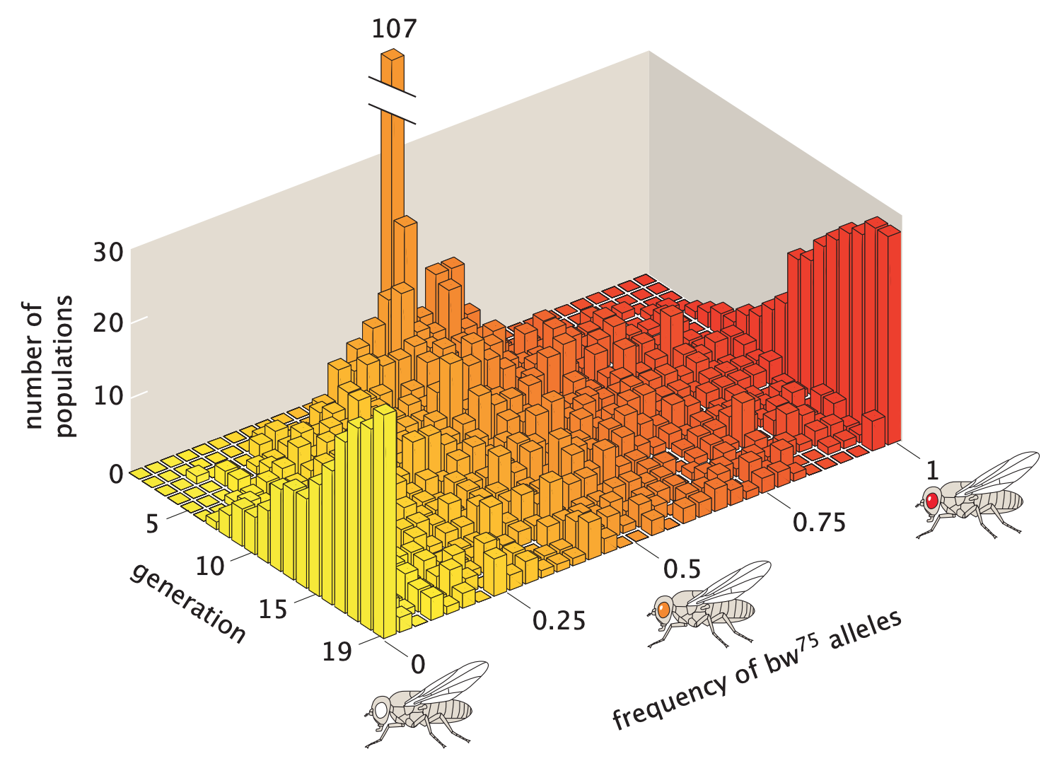
In 1956, Peter Buri used a beautiful
experiment to demonstrate this effect. Briefly, Buri began the
experiment with 107 populations of D. melanogaster (fruit fly). In each
population, the frequency of a target allele called \(\text{bw}^{75}\) is exactly 0.5. Buri
tracked the allele frequency changes over 19 generations by inferring
the genotype of each fly from its eye color. The changes in allele
frequency distribution vividly describe the effect of genetic drift on
many populations.
In the picture above, all the masses are initially concentrated at
the center. In a few generations, the masses spread out fairly evenly.
As time passes, some alleles reach fixation and some are driven out of
the population.
Derivation of forward equation
In fact, compared to our derivation, Kimura’s intuitive justification
applies to a broader class of diffusion processes, in that it doesn’t
assume time-homogeneity.
Consider a locus with a pair of alleles \(A_1\) and \(A_2\) segregating in a population. Let
\(A_1\) be the focal allele with
frequency \(p\) at time 0. Following
our notation in the previous vignette, \(\phi(p,0,x,t)\) is the transition density
for the frequency of \(A_1\), \(x\), at time \(t\). Note that we use \(\phi(\cdot)\) instead of \(p(\cdot)\) to avoid confusion between
density and initial frequency. We can further simplify our notation to
\(\phi(x,t)\) as 0 and \(p\) are both fixed quantities. The forward
equation is: \[
\frac{d}{dt}\phi(x,t) = -\frac{d}{dx}\{\phi(x,t)\mu(x, t)\} +
\frac{1}{2}\frac{d^2}{dx^2}\{\phi(x,t)\sigma^2(x,t) \}
\] Let’s pause for a second and think about the interpretation of
\(\phi(x,t)\). First of all, we
highlight the difference between diffusion process and the
characterization of genetic drift as binomial sampling (as demonstrated
in the first vignette). In the binomial sampling model, we focus on the
behavior in a single population. However, when we switch to Markov chain
and diffusion process, we are essentially modelling the average
behavior of allele frequency in many populations. Consider some
tiny \(dx > 0\), then \(\phi(x,t) dx\) can be thought of as the
proportion of populations with allele frequency \(x\) among an infinite number of “identical”
Wright-Fisher populations. Sometimes we also call \(\phi(x,t) dx\) the frequency of class \(x\) at time \(t\). In other words, think of a single
population as a small machine that runs its own drifting process. Now we
have many such population, each of which is a small machine that runs a
drifting process. Although the same set of “instructions” (parameters of
genetic drift) are sent to each machine, sampling variation in the
drifting process leads to allele frequency variation among populations.
If we pause the process at a particular time \(t\), we obtain the allele frequency
distribution at time \(t\) (as a
function of \(x\), the dummy variable
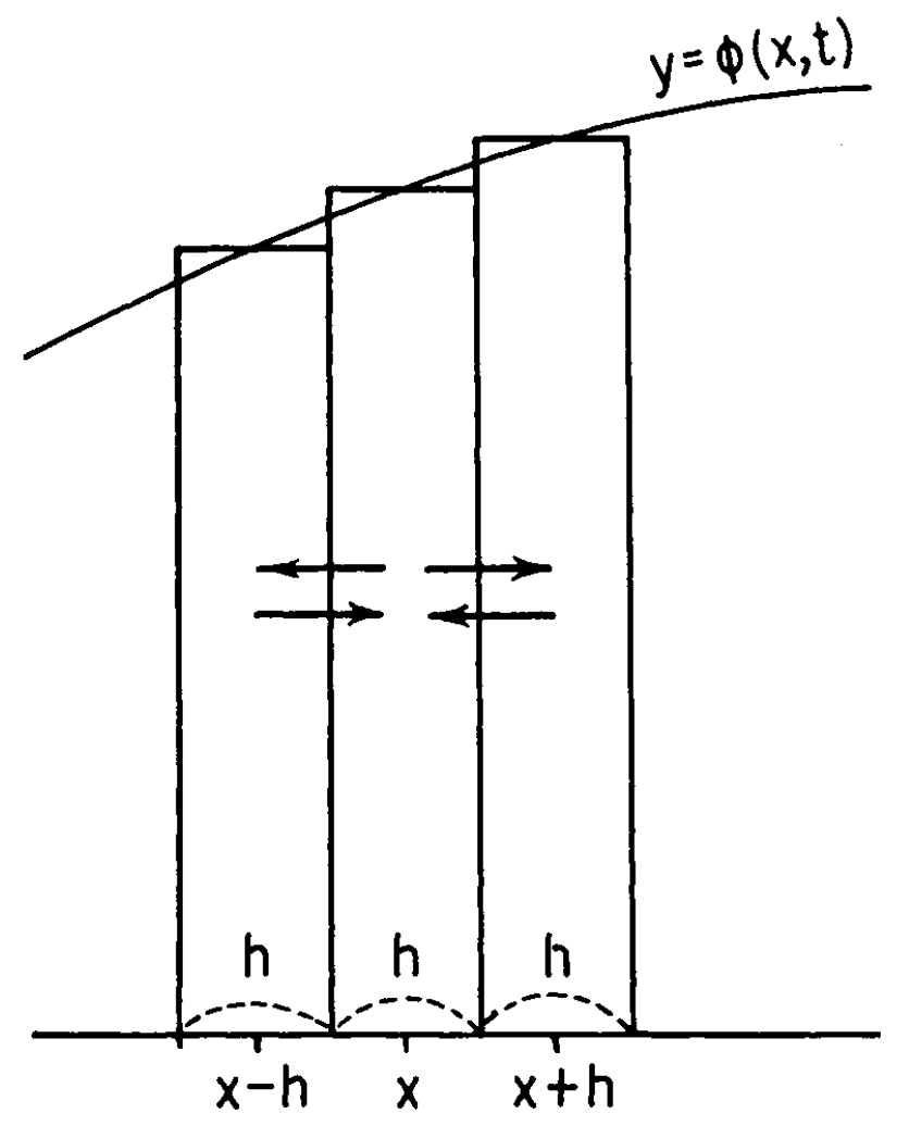
for allele frequency), which is exactly \(\phi(x,t)\). Kimura (1955) has a nice
diagram that visualizes \(\phi(x,t)\).
The distribution in approximated by bins of width \(h\). The approximation gets better as \(h\) becomes smaller, so think of \(h\) tiny. Because the density in each bin
is constant, there are only three classes here, represented by the
middle points \(x-h\), \(x\), and \(x+h\), respectively. Consider population of
allele frequency \(x\) (henthforce
class \(x\) and similarly for other
classes), we want to describe its probability of moving to another class
after some time \(\Delta t\). Recall in
the definition of diffusion process, there is a technical condition
which ensures continuous path. Therefore, if we take \(\Delta t\) sufficiently small, it will move
to either class \(x-h\) or class \(x+h\).
We also consider two forces that drive the population to different
classes: systematic pressure and randomness. Let \(m(x,t)\Delta t\) be the probability that
the population moves to class \(x+h\)
after time \(\Delta t\) due to
systematic pressure. Note that the pressure can be specified in either
direction without loss of generality. Let \(v(x,t)\Delta t\) be the probability that
the population move to a different class after time \(\Delta t\) due to randomness. Therefore, if
the population leaves the current class (say, class \(x\)) by randomness, half of time it moves
to class \(x-h\) and half of the time
to class \(x+h\). We can write the
density after time \(\Delta t\) as:
\[
\begin{aligned}
\phi(x,t+\Delta t)h &= \phi(x,t)h \\ &- [v(x,t)+m(x,t)]\Delta t
\phi(x,t)h \hspace{10mm} (\star) \\ &+ \frac{1}{2}v(x-h,t)\Delta t
\phi(x-h,t) + \frac{1}{2}v(x+h, t)\Delta t \phi(x+h,t)h \hspace{10mm}
(\star\star)\\ &+ m(x-h,t)\Delta t \phi(x-h, t)h \hspace{10mm}
(\star\star\star)
\end{aligned}
\] Let’s translate the above equation into plain English. \((\star)\) represents the probability mass
leaving class \(x\) per \(\Delta t\) at time \(t\); \((\star\star)\) represents the probability
mass moving into class \(x\) per \(\Delta t\) from the other two classes due
to randomness; \((\star\star\star)\)
represents the probability mass moving into class \(x\) per \(\Delta
t\) from class \(x-h\) by
systematic pressure (i.e.: the wind only blows from left to right).
Together, \((\star\star)\) and \((\star\star\star)\) represent the
probability mass entering class \(x\)
per \(\Delta t\) at time \(t\). Hence, the previous equation says:
\[
\begin{aligned}
\text{the probability mass in class } x \text{ at time } (t + \Delta t)
&= \text{the probability mass in class } x \text{ at time } t \\
&- \text{the probability mass leaving class } x \text{ per } \Delta
t \text{ at time } t \\ &+ \text{the probability mass entering class
} x \text{ per } \Delta t \text{ at time } t
\end{aligned}
\] Cool! Now we can define \(\sigma^2(x,t)\) and \(\mu(x,t)\). Let: \[
\begin{aligned}
\sigma^2(x,t) \Delta t &= h^2 \frac{1}{2}v(x,t)\Delta t + (-h)^2
\frac{1}{2}v(x,t)\Delta t\\
\mu(x,t) \Delta t &= hm(x,t)\Delta t
\end{aligned}
\] In other words, \(\sigma^2(x,t)
\Delta t\) is the variance of the per \(\Delta t\) change in \(x\) due to randomness, and \(\mu(x,t) \Delta t\) is the average per
\(\Delta t\) change in \(x\). Dividing both sides by \(\Delta t\), we have: \[
\begin{aligned}
\sigma^2(x,t) &= h^2 v(x,t)\\
\mu(x,t) &= hm(x,t)
\end{aligned}
\] Although \(\Delta t\) is
short, it still counts as a segment. Now we are looking at a particle.
We should interpret \(\sigma^2(x,t)\)
as the variance per infinitesimal time change in \(x\) due to randomness and \(\mu(x,t)\) the average per infinitesimal
time change in \(x\). Recall in the
definition of diffusion process, we call \(\mu(x,t)\) the infinitesimal
mean and \(\sigma^2(x,t)\) the
infinitesimal variance.
Eventually, we want to find an expression for the time derivative: \[
\lim_{\Delta t \rightarrow 0} \frac{\phi(x,t+\Delta t) -
\phi(x,t)}{\Delta t}
\] This is easy because we can substitute \(\sigma^2(x,t)\) and \(\mu(x,t)\) back to the equation for \(\phi(x,t+\Delta t)h\). With some standard
algebraic manipulations, we have the desired forward equation (remember
to take the limit as \(h \rightarrow
0\) because we start with an approximation of the distribution):
\[
\frac{d}{dt}\phi(x,t) = -\frac{d}{dx}\{\phi(x,t)\mu(x, t)\} +
\frac{1}{2}\frac{d^2}{dx^2}\{\phi(x,t)\sigma^2(x,t) \}
\]
Main reference
Stochastic processes and distribution of gene frequencies under
natural selection by Motoo Kimura (1955)