Differential expression analysis for studies with more than 2 groups

Studies with more than 2 groups (Video)

Describe the scientific question, the experimental design, and the data collected for the 3-group study. Review RNA-seq technique and the need to standardize by library size.

Calculate the library size

Use colSums to calculate the library sizes and run summary to appreciate the variability.

lib_size <- colSums(dge$counts)
summary(lib_size)

    Min.  1st Qu.   Median     Mean  3rd Qu.     Max. 
14710000 24330000 26530000 26030000 29460000 33080000 

Calculate counts per million

Use edgeR::calcNormFactors and edgeR::cpm to calculate TMM-normalized counts per million.

dge <- calcNormFactors(dge)
dge_cpm <- cpm(dge, log = TRUE)

Create density plots of counts versus counts per million

Use limma::plotDensities to visualize the distribution of counts and the distribution of counts per million.

plotDensities(dge_cpm, legend = FALSE)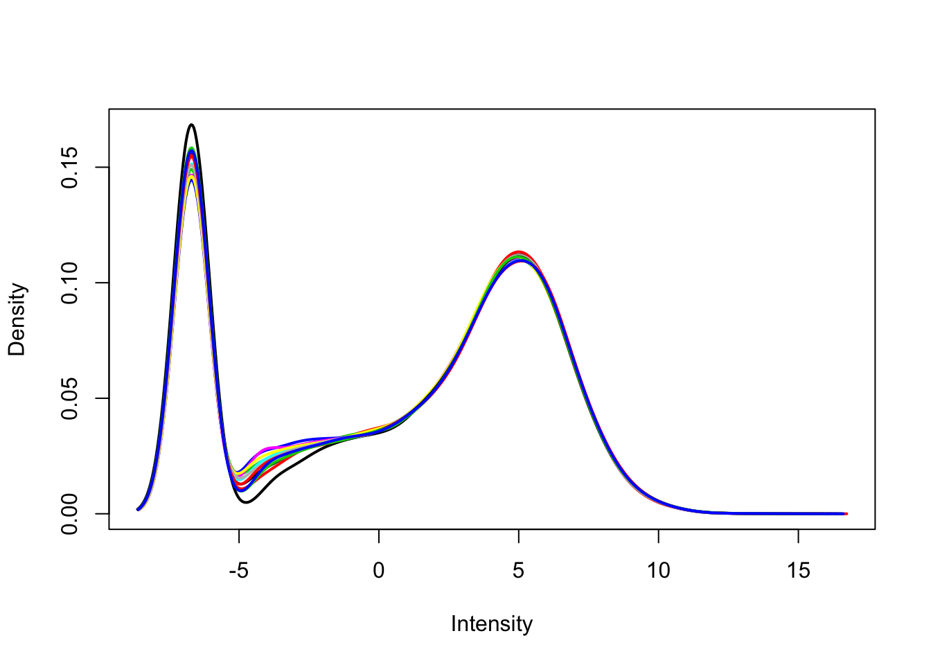

Filtering genes and samples (Video)

Describe the process of filtering lowly expressed genes (show density plots from previous exercise to demonstrate bimodal distribution) and identifying outlier samples with PCA. Discuss the nuances of removing outlier samples.

Remove lowly expressed genes

Remove any gene that does not have at least a log2 cpm > 0 in at least 4 samples (n = 4 per group). Use limma::plotDensities to confirm the distribution of counts per million is unimodal post-filtering.

dge_filt <- dge[rowSums(dge_cpm > 0) >= 4, ]
dge_filt <- calcNormFactors(dge_filt)
dge_filt_cpm <- cpm(dge_filt, log = TRUE)
plotDensities(dge_filt_cpm, legend = FALSE)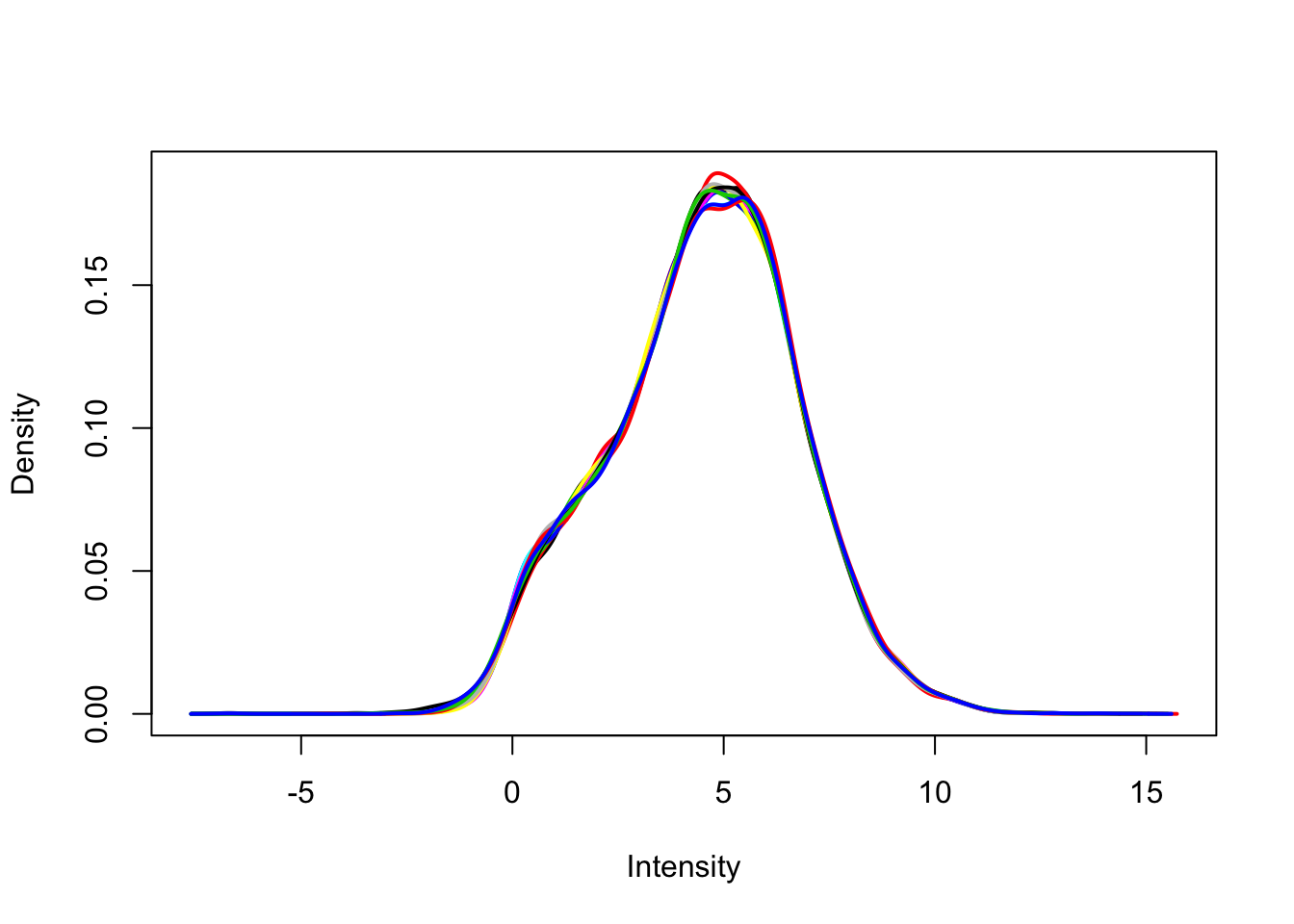

Use PCA to identify outlier sample

Use prcomp to calculate PCA and then plot PC1 vs. PC2. Remove the exgf sample that clusters with the gf samples.

pca <- prcomp(t(dge_filt_cpm), scale. = TRUE)
plot(pca)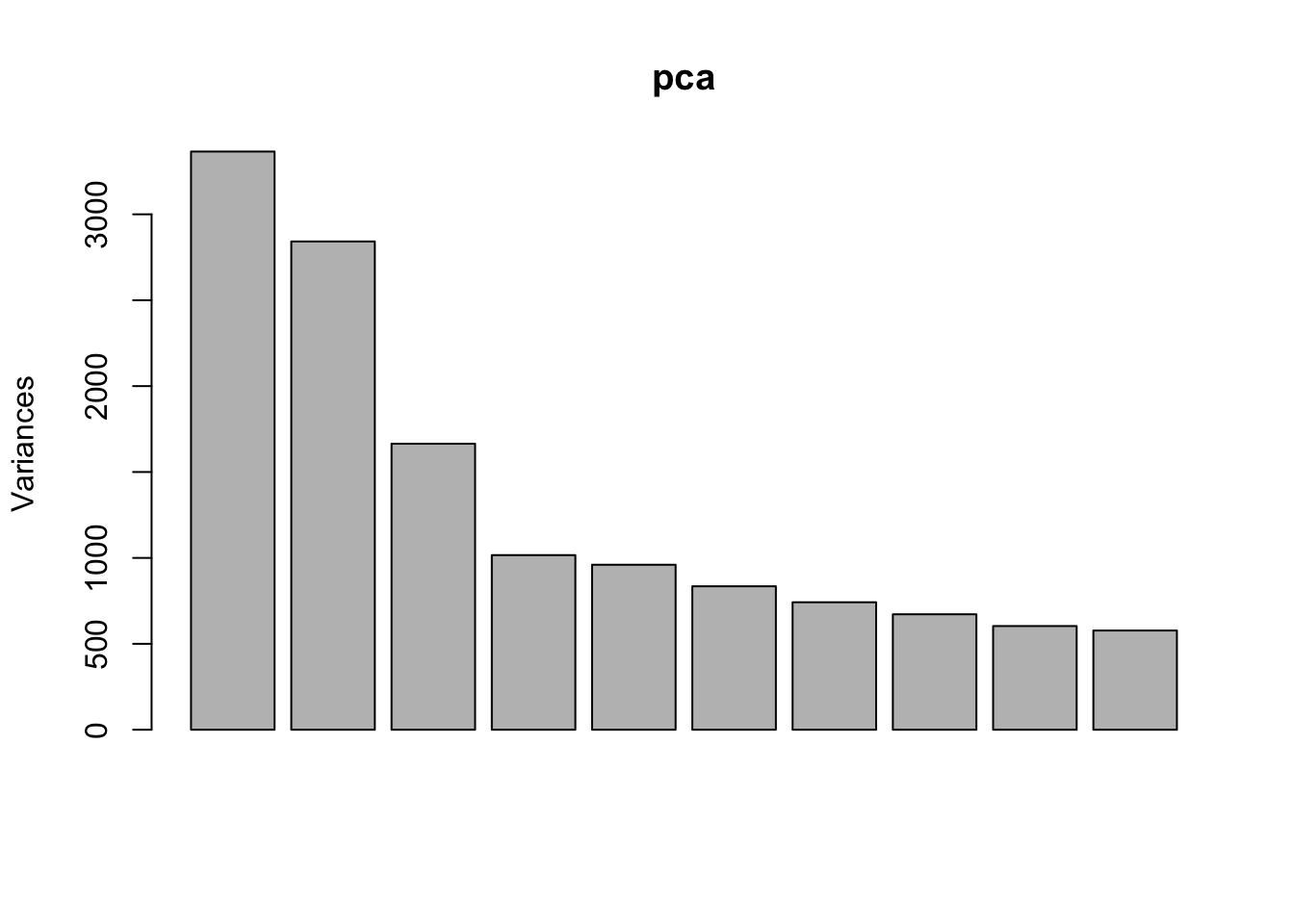

d <- data.frame(dge_filt$samples, pca$x)
ggplot(d, aes(x = PC1, y = PC2, color = group)) +
  geom_text(aes(label = id))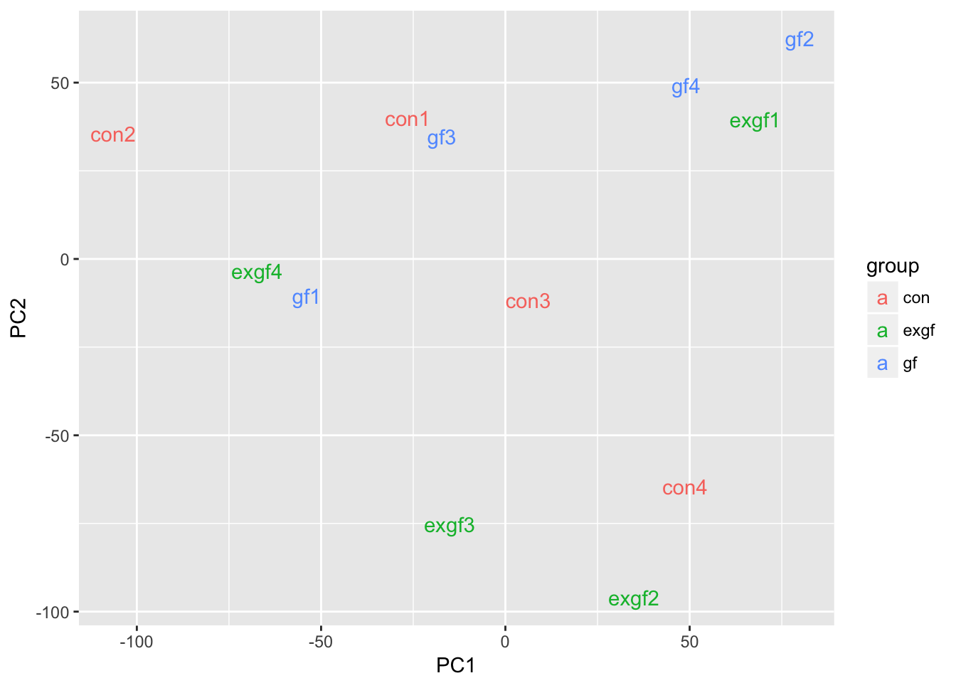

plotMDS(dge_filt)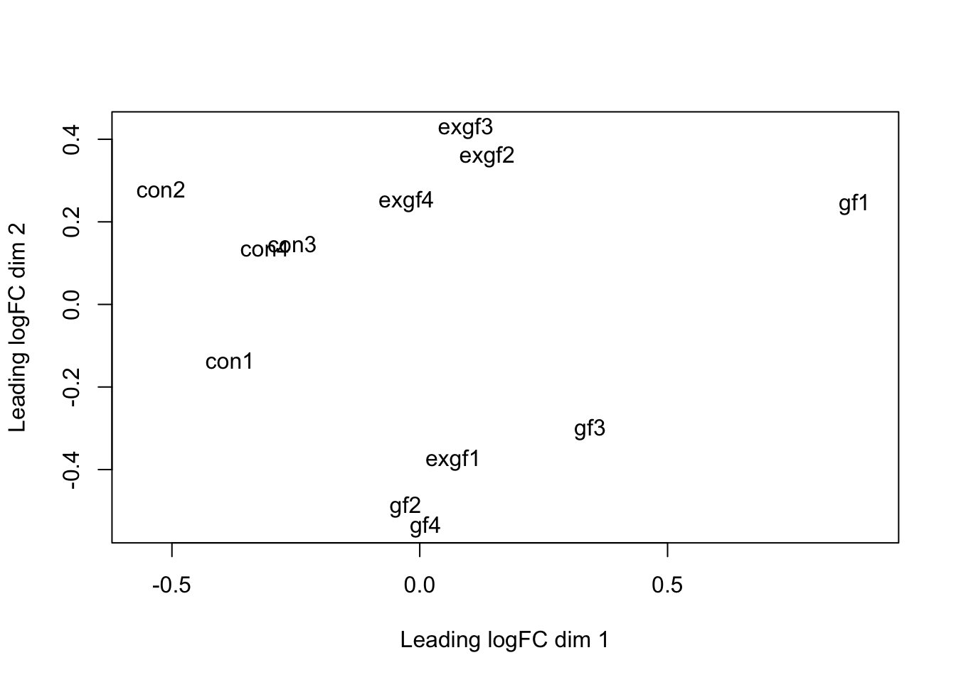

dge_final <- dge_filt[, dge_filt$samples$id != "exgf1"]

Differential expression for RNA-seq with voom (Video)

Review how to use model.matrix and limma::makeContrasts. Describe how limma::voom corrects for the mean-variance relationship of the count data.

Create design matrix for study with 3 groups

Use model.matrix to create a linear model with three binary variables (group-means parametrization).

design <- model.matrix(~0 + group, data = dge_final$samples)
colnames(design) <- str_replace(colnames(design), "group", "")
colSums(design)

 con exgf   gf 
   4    3    4 

Create contrasts matrix for study with 3 groups

Use limma::makeContrasts to test all pairwise comparisions.

cont_mat <- makeContrasts(gf.con = gf - con,
                          exgf.con = exgf - con,
                          exgf.gf = exgf - gf,
                          levels = design)
cont_mat

      Contrasts
Levels gf.con exgf.con exgf.gf
  con      -1       -1       0
  exgf      0        1       1
  gf        1        0      -1

Account for mean-variance relationship with voom

Use limma::voom to calculate weights for the linear model to account for the mean-variance relationship of the counts. Set plot = TRUE to visualize the mean-variance trend. Explore the EList object returned to confirm that the expression values in E are simply the counts per million.

dge_final <- calcNormFactors(dge_final)
v <- voom(dge_final, design, plot = TRUE)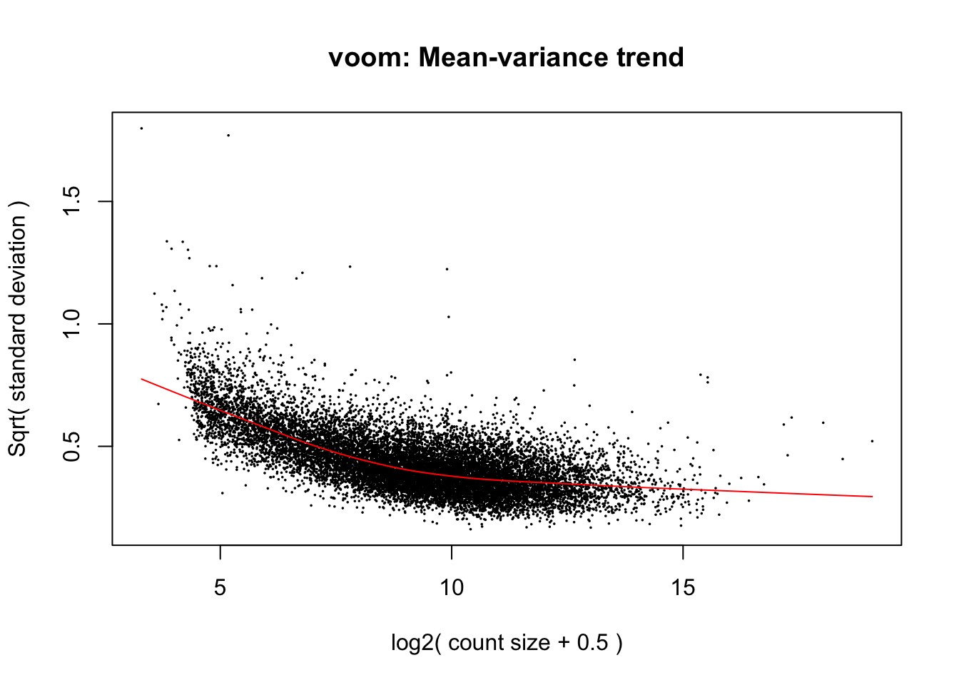

plotDensities(v$E, legend = FALSE)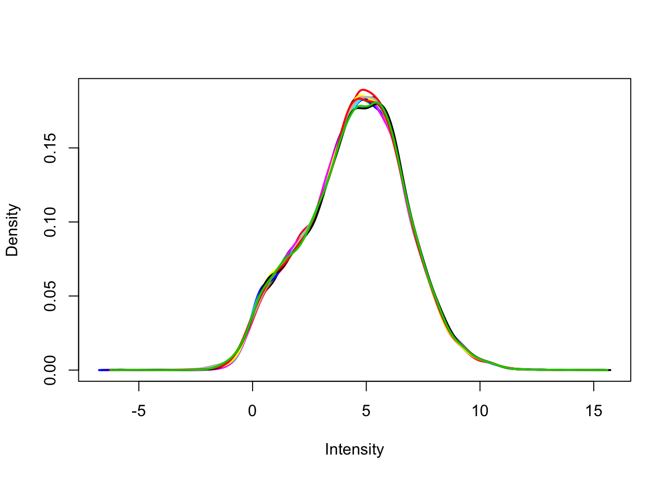

dge_final_cpm <- cpm(dge_final, log = TRUE)
plot(v$E[, 1], dge_final_cpm[, 1])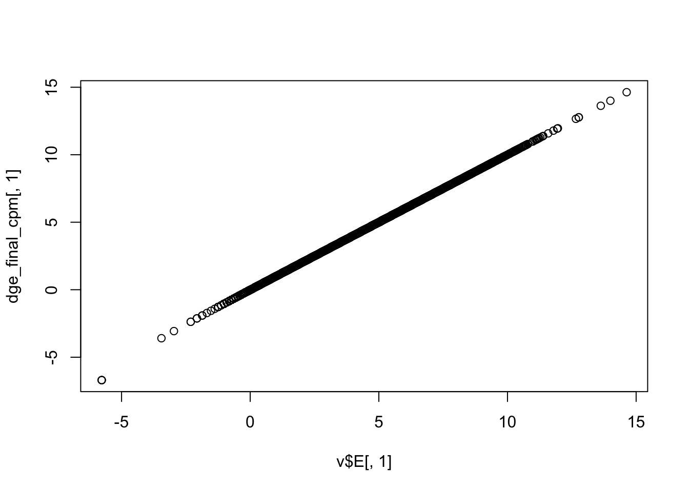

Fit and test model for study with 3 groups

Use limma::lmFit, limma::contrasts.fit, limma::eBayes, and limma::decideTests to fit and test the model. Use limma::vennDiagram to visualize overlap of differentially expressed genes.

fit <- lmFit(v, design)
fit2 <- contrasts.fit(fit, contrasts = cont_mat)
fit2 <- eBayes(fit2)
results <- decideTests(fit2)
vennDiagram(results)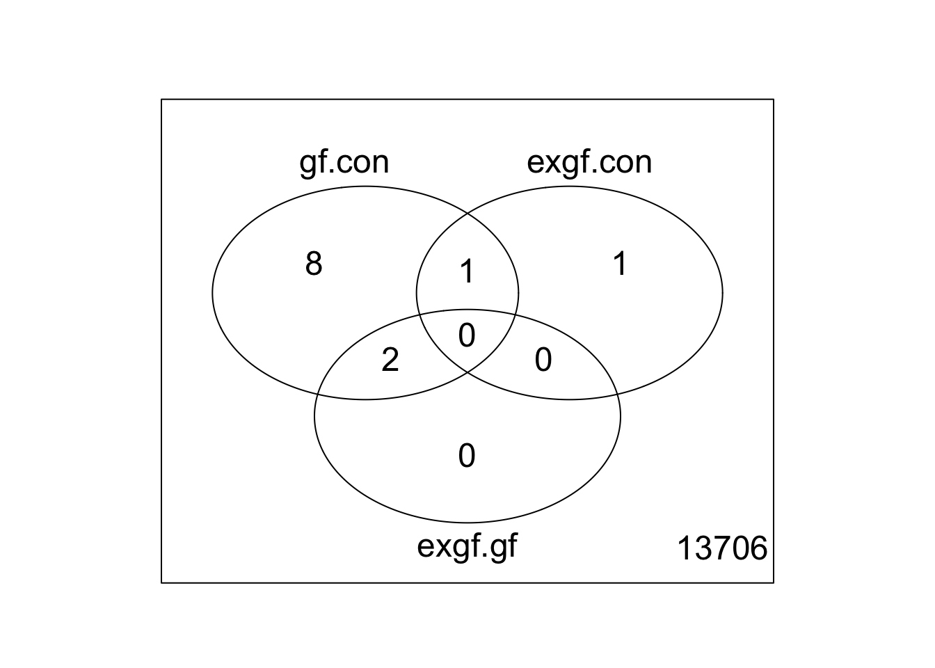

Session information

sessionInfo()

R version 3.3.2 (2016-10-31)
Platform: x86_64-apple-darwin13.4.0 (64-bit)
Running under: OS X Yosemite 10.10.5

locale:
[1] en_US.UTF-8/en_US.UTF-8/en_US.UTF-8/C/en_US.UTF-8/en_US.UTF-8

attached base packages:
[1] parallel  stats     graphics  grDevices utils     datasets  methods  
[8] base     

other attached packages:
[1] stringr_1.2.0       ggplot2_2.2.1       edgeR_3.16.5       
[4] limma_3.30.13       Biobase_2.34.0      BiocGenerics_0.20.0

loaded via a namespace (and not attached):
 [1] Rcpp_0.12.11     knitr_1.18       magrittr_1.5     munsell_0.4.3   
 [5] colorspace_1.3-2 lattice_0.20-34  rlang_0.1.6      plyr_1.8.4      
 [9] tools_3.3.2      grid_3.3.2       gtable_0.2.0     git2r_0.20.0    
[13] htmltools_0.3.6  lazyeval_0.2.1   yaml_2.1.16      rprojroot_1.2   
[17] digest_0.6.13    tibble_1.3.3     evaluate_0.10.1  rmarkdown_1.8   
[21] labeling_0.3     stringi_1.1.5    scales_0.4.1     backports_1.1.0 
[25] locfit_1.5-9.1