Differential expression analysis for studies with a 2x2 factorial design

Last updated: 2018-06-15

workflowr checks: (Click a bullet for more information)

✔ R Markdown file: up-to-date

Great! Since the R Markdown file has been committed to the Git repository, you know the exact version of the code that produced these results.
✔ Environment: empty

Great job! The global environment was empty. Objects defined in the global environment can affect the analysis in your R Markdown file in unknown ways. For reproduciblity it’s best to always run the code in an empty environment.
✔ Seed: set.seed(12345)

The command set.seed(12345) was run prior to running the code in the R Markdown file. Setting a seed ensures that any results that rely on randomness, e.g. subsampling or permutations, are reproducible.
✔ Session information: recorded

Great job! Recording the operating system, R version, and package versions is critical for reproducibility.
✔ Repository version: d979358
Great! You are using Git for version control. Tracking code development and connecting the code version to the results is critical for reproducibility. The version displayed above was the version of the Git repository at the time these results were generated.

Note that you need to be careful to ensure that all relevant files for the analysis have been committed to Git prior to generating the results (you can use wflow_publish or wflow_git_commit). workflowr only checks the R Markdown file, but you know if there are other scripts or data files that it depends on. Below is the status of the Git repository when the results were generated:
```
Ignored files:
    Ignored:    .Rhistory
    Ignored:    .Rproj.user/

Untracked files:
    Untracked:  code/counts_per_sample.txt
    Untracked:  code/table-s1.txt
```
Note that any generated files, e.g. HTML, png, CSS, etc., are not included in this status report because it is ok for generated content to have uncommitted changes.

Expand here to see past versions:

File	Version	Author	Date	Message
Rmd	d979358	John Blischak	2018-06-15	Use all lowercase variables for dox phenotypes.
Rmd	c361225	John Blischak	2018-05-30	Experiment with normalizing and filtering doxorubicin data.
html	9b58c25	John Blischak	2018-05-23	Build site.
html	79a1ea4	John Blischak	2018-05-23	Build site.
Rmd	3e36241	John Blischak	2018-05-23	Update to 1.0
html	3e36241	John Blischak	2018-05-23	Update to 1.0
html	67f13a4	John Blischak	2018-03-09	Build site.
Rmd	a2fc9a7	John Blischak	2018-03-09	Minor edits to ch04 solutions
html	b2dc653	John Blischak	2018-01-25	Build site.
Rmd	dc82382	John Blischak	2018-01-25	Minor updates to Ch 04 analysis.
html	7f4d46b	John Blischak	2018-01-11	Build site.
Rmd	5db0175	John Blischak	2018-01-11	Organize Ch 04

Analayze microarray data from Zhang et al., 2012, which measured gene expression in hearts from wild type and Top2b null mice treated with doxorubicin or a control.

library("Biobase")
library("ggplot2")
library("limma")
eset <- readRDS("../data/ch04.rds")

Studies with a 2x2 factorial design (Video)

Describe the scientific question, the experimental design, and the data collected for the 2x2 factorial study.

Expression level of Top2b

Create a boxplot of the expression level of Top2b to confirm the null mice have lower levels of Top2b expression. Use pData and table to access and explore the phenotype measurements to be used in the plot.

head(fData(eset))

           probe chrom     start       end symbol            ensembl
1  A_55_P2051983 chr18  62753954  62753895 Spink7 ENSMUST00000076194
2   A_52_P169082 chr11  76031955  76032014  Dbil5                   
3 A_30_P01028193 chr14  47982421  47982480                          
4   A_52_P237997  chr3 156834624 156834683  Negr1                   
5   A_51_P414243  chr9 121890800 121890741 C85492 ENSMUST00000084743
6  A_55_P2136348  chr9 120003293 120003352   Ccr8 ENSMUST00000048777
        refseq entrez                                                name
1 NM_001001803 408198 serine peptidase inhibitor, Kazal type 7 (putative)
2    NM_021294  13168                   diazepam binding inhibitor-like 5
3                  NA                                                    
4    NM_177274 320840                         neuronal growth regulator 1
5    NM_153540 215494                           expressed sequence C85492
6    NM_007720  12776                    chemokine (C-C motif) receptor 8

top2b <- exprs(eset)[fData(eset)$symbol == "Top2b", ]
head(pData(eset))

                                                  title genotype treatment
wt.pbs.r1         WT Cardiomyocytes 16hr after PBS rep1       wt       pbs
wt.pbs.r2         WT Cardiomyocytes 16hr after PBS rep2       wt       pbs
wt.pbs.r3         WT Cardiomyocytes 16hr after PBS rep3       wt       pbs
wt.dox.r1 WT Cardiomyocytes 16hr after doxorubicin rep1       wt       dox
wt.dox.r2 WT Cardiomyocytes 16hr after doxorubicin rep2       wt       dox
wt.dox.r3 WT Cardiomyocytes 16hr after doxorubicin rep3       wt       dox
          rep
wt.pbs.r1  r1
wt.pbs.r2  r2
wt.pbs.r3  r3
wt.dox.r1  r1
wt.dox.r2  r2
wt.dox.r3  r3

d <- data.frame(pData(eset), top2b)
ggplot(d, aes(x = treatment, y = top2b, fill = genotype)) +
  geom_boxplot()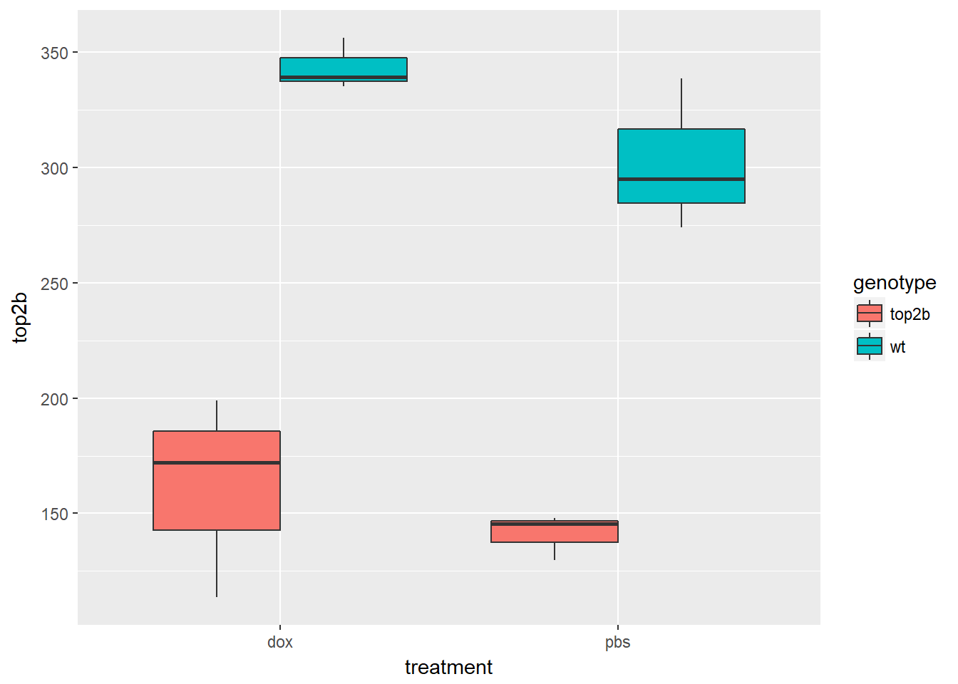

Expand here to see past versions of unnamed-chunk-1-1.png:

Version	Author	Date
67f13a4	John Blischak	2018-03-09
b2dc653	John Blischak	2018-01-25
7f4d46b	John Blischak	2018-01-11

Visualize gene expression distribution with boxplots

Use boxplots as an alternative to density plots for checking the distribution of gene expression levels. Note pro (easier to see which sample belongs to each distribution) and con (hides any multimodality).

boxplot(exprs(eset))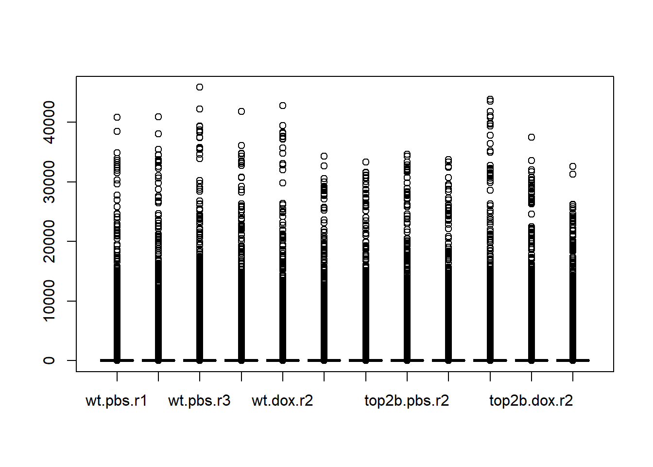

Expand here to see past versions of unnamed-chunk-2-1.png:

Version	Author	Date
67f13a4	John Blischak	2018-03-09
b2dc653	John Blischak	2018-01-25
7f4d46b	John Blischak	2018-01-11

boxplot(log(exprs(eset)))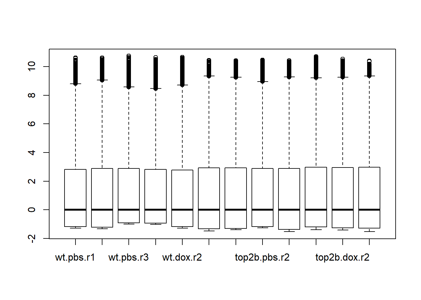

Expand here to see past versions of unnamed-chunk-2-2.png:

Version	Author	Date
67f13a4	John Blischak	2018-03-09

boxplot(log(exprs(eset)), las = 2)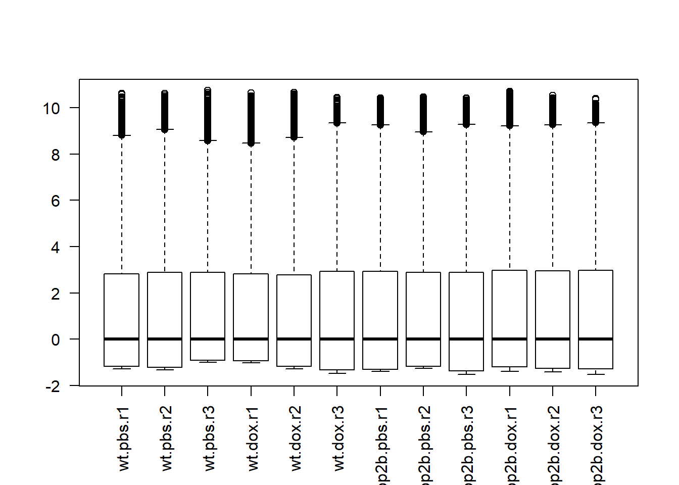

Expand here to see past versions of unnamed-chunk-2-3.png:

Version	Author	Date
67f13a4	John Blischak	2018-03-09

plotDensities(log(exprs(eset)), group = pData(eset)$genotype, legend = "topright")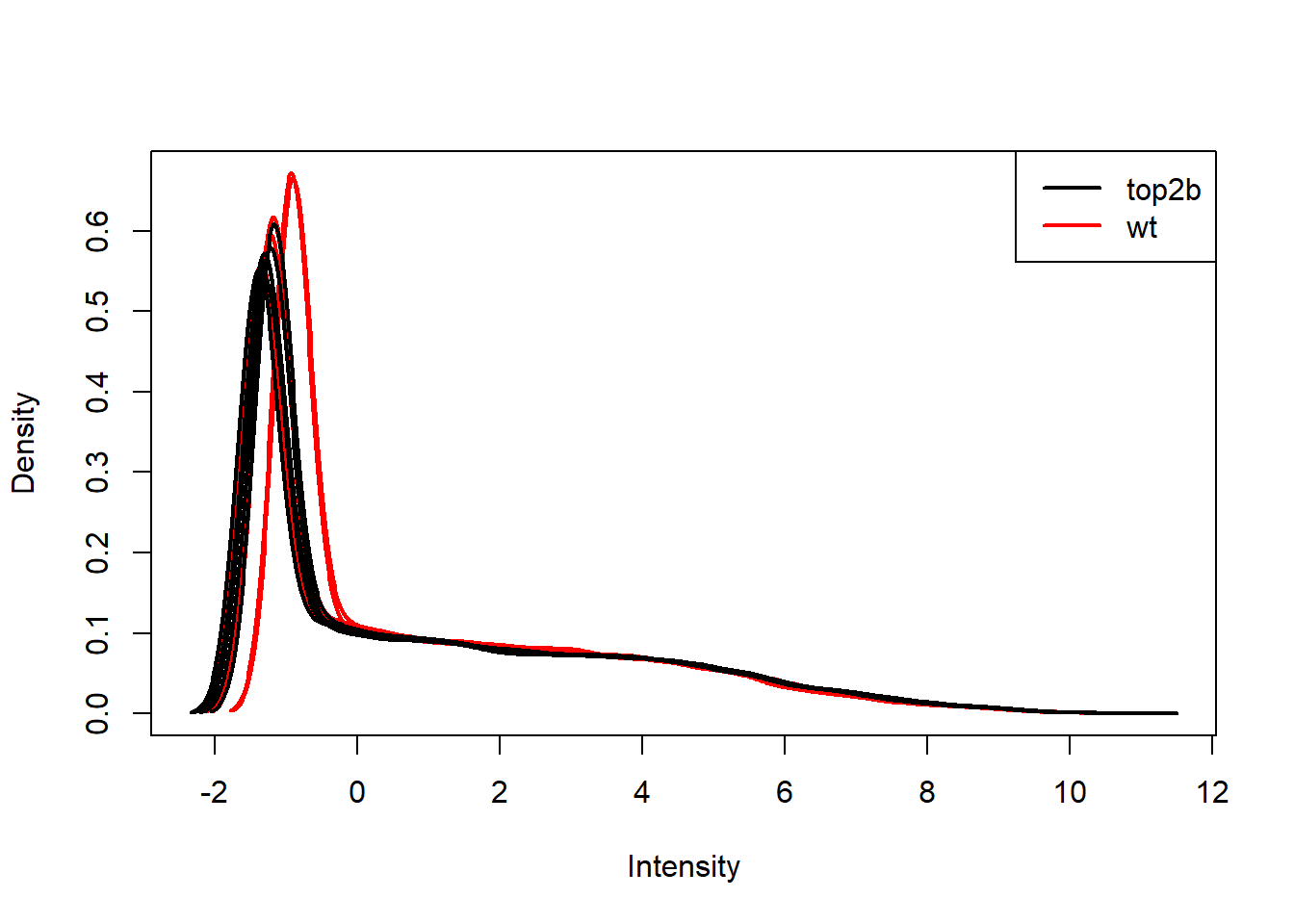

exprs(eset) <- normalizeBetweenArrays(log(exprs(eset)))
plotDensities(exprs(eset), group = pData(eset)$genotype, legend = "topright")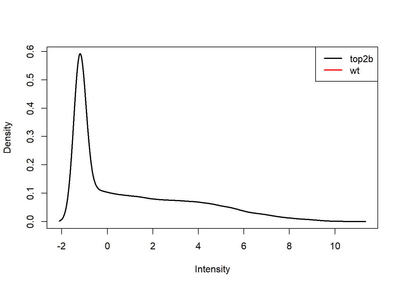

eset <- eset[rowMeans(exprs(eset)) > 0, ]
dim(eset)

Features  Samples 
   28965       12

plotDensities(exprs(eset), group = pData(eset)$genotype, legend = "topright")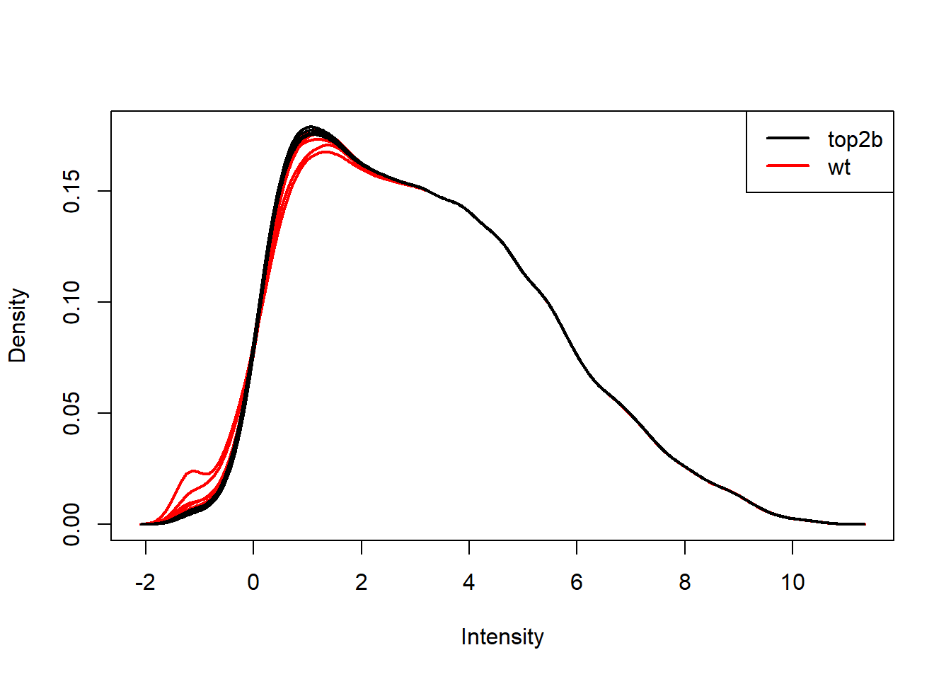

Perform PCA

Use prcomp to calculate PCs and plot PC2 vs. PC1 to confirm that the samples are separated by genotype and treatment. Note that Top2b mice all cluster with untreated WT samples since they are resistant to the treatment.

pca <- prcomp(t(exprs(eset)), scale. = TRUE)
plot(pca)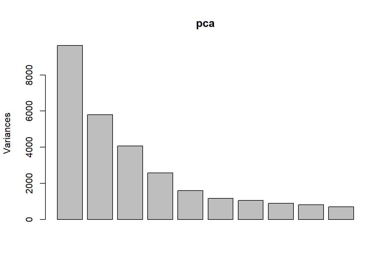

Expand here to see past versions of unnamed-chunk-3-1.png:

Version	Author	Date
67f13a4	John Blischak	2018-03-09
b2dc653	John Blischak	2018-01-25
7f4d46b	John Blischak	2018-01-11

d <- data.frame(pData(eset), pca$x)
ggplot(d, aes(x = PC1, y = PC2, color = genotype, shape = treatment)) +
  geom_point()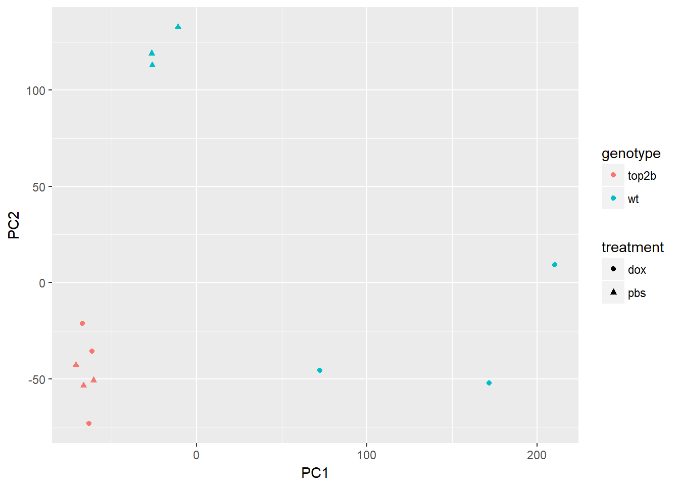

Expand here to see past versions of unnamed-chunk-3-2.png:

Version	Author	Date
67f13a4	John Blischak	2018-03-09
b2dc653	John Blischak	2018-01-25
7f4d46b	John Blischak	2018-01-11

ggplot(d, aes(x = treatment, y = PC1, fill = genotype)) +
  geom_boxplot()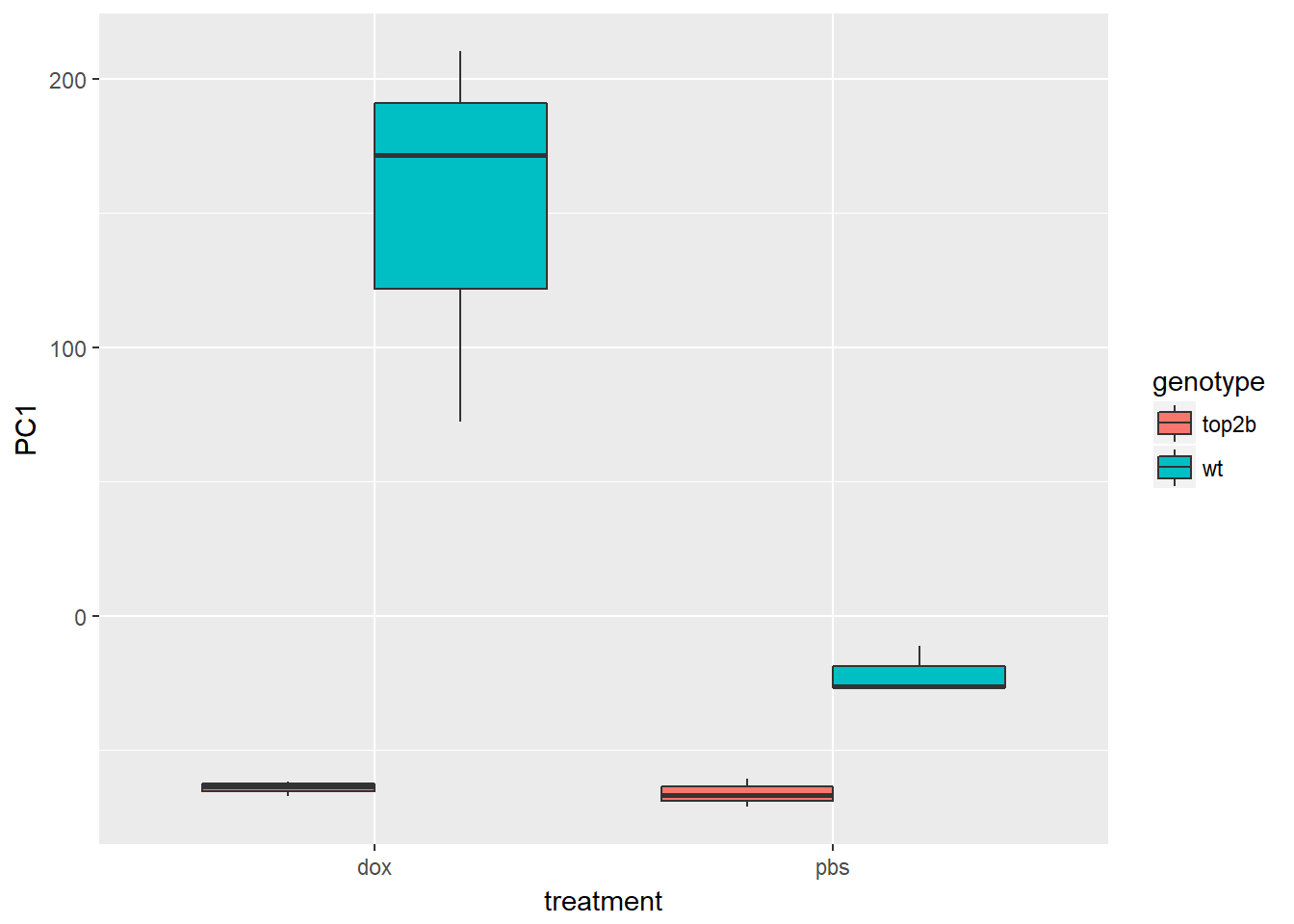

Expand here to see past versions of unnamed-chunk-3-3.png:

Version	Author	Date
67f13a4	John Blischak	2018-03-09
b2dc653	John Blischak	2018-01-25
7f4d46b	John Blischak	2018-01-11

ggplot(d, aes(x = treatment, y = PC2, fill = genotype)) +
  geom_boxplot()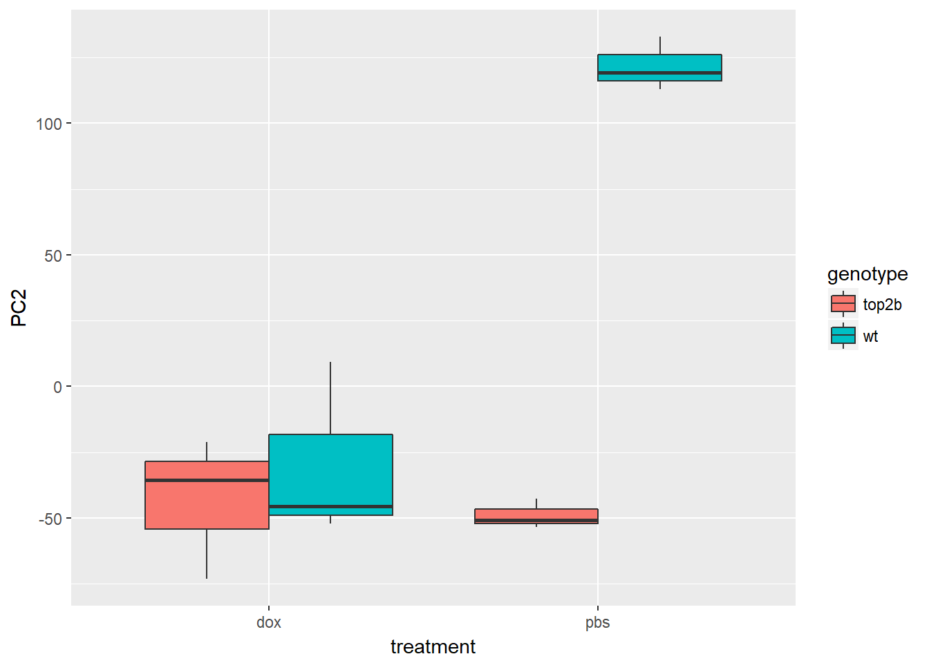

Expand here to see past versions of unnamed-chunk-3-4.png:

Version	Author	Date
67f13a4	John Blischak	2018-03-09
b2dc653	John Blischak	2018-01-25
7f4d46b	John Blischak	2018-01-11

Differential expression for 2x2 factorial designs (Video)

Discuss how to construct a design and contrasts matrix for a 2x2 factorial design. Note how to create a combined factor and how to write the contrast for the interaction term.

Create design matrix for 2x2 factorial design

Create a combined factor using paste. Use model.matrix to create a linear model with 4 binary variables (group-means parametrization).

f <- paste(pData(eset)$genotype, pData(eset)$treatment, sep = ".")
design <- model.matrix(~0 + f)
colnames(design) <- sub("f", "", colnames(design))
colSums(design)

top2b.dox top2b.pbs    wt.dox    wt.pbs 
        3         3         3         3

Create contrasts matrix for 2x2 factorial design

Use limma::makeContrasts to test the main effects and the interaction between genotype and treatment.

cont_mat <- makeContrasts(DoxWT = wt.dox - wt.pbs,
                          DoxTop = top2b.dox - top2b.pbs,
                          Interaction = (top2b.dox - top2b.pbs) -
                                        (wt.dox - wt.pbs),
                          levels = design)
cont_mat

           Contrasts
Levels      DoxWT DoxTop Interaction
  top2b.dox     0      1           1
  top2b.pbs     0     -1          -1
  wt.dox        1      0          -1
  wt.pbs       -1      0           1

Fit and test 2x2 factorial design

Use limma::lmFit, limma::contrasts.fit, limma::eBayes, and limma::decideTests to fit and test the model. Use limma::vennDiagram to visualize overlap of differentially expressed genes.

fit <- lmFit(eset, design)
head(fit$coefficients)

   top2b.dox top2b.pbs   wt.dox   wt.pbs
2   1.405056  1.536537 1.280498 1.172957
5   5.479908  5.486018 5.628112 5.656115
10  1.987281  1.913208 2.206463 2.162715
11  5.688783  5.789735 5.314792 5.283211
14  5.384812  5.406607 5.181832 5.499237
15  1.876791  1.809405 1.765531 1.833199

fit2 <- contrasts.fit(fit, contrasts = cont_mat)
head(fit2$coefficients)

    Contrasts
           DoxWT       DoxTop Interaction
  2   0.10754056 -0.131481235 -0.23902179
  5  -0.02800370 -0.006109353  0.02189435
  10  0.04374777  0.074073731  0.03032596
  11  0.03158122 -0.100951885 -0.13253311
  14 -0.31740484 -0.021795427  0.29560942
  15 -0.06766808  0.067386526  0.13505461

fit2 <- eBayes(fit2)
results <- decideTests(fit2)
summary(results)

       DoxWT DoxTop Interaction
Down    4235      0        1427
NotSig 20857  28965       25687
Up      3873      0        1851

vennDiagram(results)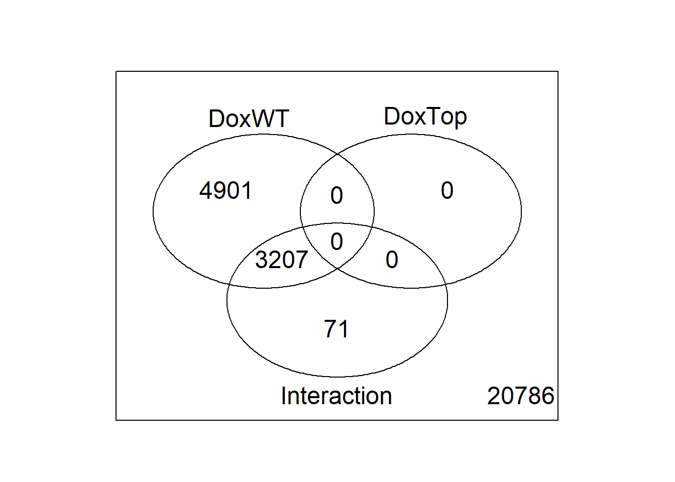

Expand here to see past versions of unnamed-chunk-6-1.png:

Version	Author	Date
67f13a4	John Blischak	2018-03-09
b2dc653	John Blischak	2018-01-25
7f4d46b	John Blischak	2018-01-11

Enrichment analysis (Video)

Describe common approaches for testing for enrichment of gene sets. Discuss Gene Onotlogy categories and KEGG pathways. Introduce Fisher’s Exact Test. Stress the importance of choosing the correct background set of genes and caution against over-interpretation (especially for directional effect). Mention at the end that there are more sophisticated algorithms such as limma::camera, limma::roast, and goseq::goseq.

Enrichment of KEGG pathways

Use limma::kegga and limma::topKEGG to test for enrichment of differentially expressed genes in KEGG pathways.

entrez <- fit2$genes$entrez
enrich_kegg_wt <- kegga(fit2, coef = "DoxWT",
                        geneid = entrez, species = "Mm")
topKEGG(enrich_kegg_wt)

                                                             Pathway   N
path:mmu05322                           Systemic lupus erythematosus  76
path:mmu05034                                             Alcoholism 130
path:mmu05330                                    Allograft rejection  26
path:mmu05412 Arrhythmogenic right ventricular cardiomyopathy (ARVC)  52
path:mmu03008                      Ribosome biogenesis in eukaryotes  71
path:mmu05332                              Graft-versus-host disease  28
path:mmu05203                                   Viral carcinogenesis 172
path:mmu04940                               Type I diabetes mellitus  31
path:mmu04261                 Adrenergic signaling in cardiomyocytes 113
path:mmu04137                                     Mitophagy - animal  62
path:mmu04020                              Calcium signaling pathway 125
path:mmu04217                                            Necroptosis 134
path:mmu05320                             Autoimmune thyroid disease  34
path:mmu04974                       Protein digestion and absorption  47
path:mmu04022                             cGMP-PKG signaling pathway 131
path:mmu05168                               Herpes simplex infection 159
path:mmu04919                      Thyroid hormone signaling pathway 104
path:mmu04612                    Antigen processing and presentation  53
path:mmu05167      Kaposi's sarcoma-associated herpesvirus infection 158
path:mmu04115                                  p53 signaling pathway  60
              Up Down         P.Up       P.Down
path:mmu05322 37    1 2.587115e-11 9.999998e-01
path:mmu05034 46   17 4.415300e-08 9.586496e-01
path:mmu05330 16    0 1.786229e-07 1.000000e+00
path:mmu05412  1   26 9.998834e-01 2.255483e-07
path:mmu03008 29    4 4.415352e-07 9.995765e-01
path:mmu05332 16    0 7.420483e-07 1.000000e+00
path:mmu05203 51   22 4.226308e-06 9.811657e-01
path:mmu04940 16    0 4.532716e-06 1.000000e+00
path:mmu04261 13   40 9.282700e-01 1.261940e-05
path:mmu04137 24   12 1.285527e-05 4.727691e-01
path:mmu04020 10   43 9.972075e-01 1.381343e-05
path:mmu04217 41   21 1.568944e-05 8.220904e-01
path:mmu05320 16    1 2.057586e-05 9.990078e-01
path:mmu04974  2   21 9.972219e-01 2.969888e-05
path:mmu04022  9   43 9.994705e-01 5.002701e-05
path:mmu05168 45   21 5.406625e-05 9.681379e-01
path:mmu04919 12   36 9.195045e-01 5.790107e-05
path:mmu04612 20    6 1.015832e-04 9.419283e-01
path:mmu05167 43   26 2.058751e-04 7.649225e-01
path:mmu04115 21    6 2.376781e-04 9.751968e-01

enrich_kegg_inter <- kegga(fit2, coef = "Interaction",
                        geneid = entrez, species = "Mm")
topKEGG(enrich_kegg_inter)

                                                                 Pathway
path:mmu05322                               Systemic lupus erythematosus
path:mmu05034                                                 Alcoholism
path:mmu03008                          Ribosome biogenesis in eukaryotes
path:mmu05412     Arrhythmogenic right ventricular cardiomyopathy (ARVC)
path:mmu04115                                      p53 signaling pathway
path:mmu04217                                                Necroptosis
path:mmu05414                               Dilated cardiomyopathy (DCM)
path:mmu05203                                       Viral carcinogenesis
path:mmu05202                    Transcriptional misregulation in cancer
path:mmu05410                          Hypertrophic cardiomyopathy (HCM)
path:mmu00534 Glycosaminoglycan biosynthesis - heparan sulfate / heparin
path:mmu03013                                              RNA transport
path:mmu05142                  Chagas disease (American trypanosomiasis)
path:mmu04012                                     ErbB signaling pathway
path:mmu04137                                         Mitophagy - animal
path:mmu05152                                               Tuberculosis
path:mmu03040                                                Spliceosome
path:mmu04020                                  Calcium signaling pathway
path:mmu05205                                    Proteoglycans in cancer
path:mmu04015                                     Rap1 signaling pathway
                N Up Down         P.Up       P.Down
path:mmu05322  76  0   25 1.000000e+00 3.607857e-12
path:mmu05034 130 10   26 6.492511e-01 1.694044e-07
path:mmu03008  71  0   18 1.000000e+00 3.436244e-07
path:mmu05412  52 16    1 2.785106e-06 9.682854e-01
path:mmu04115  60  2   13 9.651619e-01 8.707340e-05
path:mmu04217 134  9   21 7.940145e-01 1.197793e-04
path:mmu05414  68 15    2 3.830266e-04 9.378625e-01
path:mmu05203 172  7   23 9.909773e-01 6.317987e-04
path:mmu05202 132  8   19 8.680539e-01 7.408914e-04
path:mmu05410  65 14    2 7.650457e-04 9.269001e-01
path:mmu00534  17  6    0 1.818698e-03 1.000000e+00
path:mmu03013 150  7   19 9.710062e-01 3.371750e-03
path:mmu05142  80  7   12 5.027586e-01 4.754486e-03
path:mmu04012  71 13    4 5.281088e-03 6.753477e-01
path:mmu04137  62  6   10 4.131237e-01 5.709701e-03
path:mmu05152 125 14   16 1.562344e-01 6.155321e-03
path:mmu03040 127  7   16 9.124164e-01 7.164024e-03
path:mmu04020 125 19    4 7.375150e-03 9.630814e-01
path:mmu05205 161 23   14 7.375432e-03 1.514618e-01
path:mmu04015 162 23    3 7.940031e-03 9.984658e-01

Enrichment of Gene Ontology categories

Use limma::goana and limma::topGO to test for enrichment of differentially expressed genes in Gene Ontology categories.

enrich_go_wt <- goana(fit2, coef = "DoxWT",
                      geneid = entrez, species = "Mm")
topGO(enrich_go_wt, ontology = "BP")

                                                       Term Ont     N   Up
GO:0090304                   nucleic acid metabolic process  BP  3705  764
GO:0016070                            RNA metabolic process  BP  3315  693
GO:0010467                                  gene expression  BP  3925  784
GO:0006396                                   RNA processing  BP   756  201
GO:0022613             ribonucleoprotein complex biogenesis  BP   387  119
GO:0042254                              ribosome biogenesis  BP   259   89
GO:0043170                  macromolecule metabolic process  BP  6446 1185
GO:0006139 nucleobase-containing compound metabolic process  BP  4135  804
GO:0034641     cellular nitrogen compound metabolic process  BP  4688  889
GO:0046483                    heterocycle metabolic process  BP  4225  810
GO:0006725     cellular aromatic compound metabolic process  BP  4258  813
GO:0007507                                heart development  BP   470   51
GO:0006364                                  rRNA processing  BP   177   63
GO:0008150                               biological_process  BP 13081 2074
GO:0034470                                 ncRNA processing  BP   314   94
GO:0060047                                heart contraction  BP   168   16
GO:0008016                  regulation of heart contraction  BP   136   13
GO:1901360        organic cyclic compound metabolic process  BP  4376  822
GO:0034097                             response to cytokine  BP   587  150
GO:0003015                                    heart process  BP   170   16
           Down         P.Up       P.Down
GO:0090304  615 5.725046e-19 9.997482e-01
GO:0016070  564 2.401108e-18 9.940679e-01
GO:0010467  682 1.096219e-15 9.828279e-01
GO:0006396  127 1.214908e-14 8.980481e-01
GO:0022613   51 1.369773e-13 9.980823e-01
GO:0042254   22 1.801469e-13 9.999983e-01
GO:0043170 1180 2.782282e-13 6.847707e-01
GO:0006139  724 4.147439e-13 9.730518e-01
GO:0034641  828 5.672903e-12 9.621104e-01
GO:0046483  752 9.985001e-12 9.147832e-01
GO:0006725  757 2.323034e-11 9.222017e-01
GO:0007507  144 9.994974e-01 6.030905e-11
GO:0006364   17 1.170328e-10 9.996583e-01
GO:0008150 2477 9.389315e-01 2.515467e-10
GO:0034470   44 2.636398e-10 9.858074e-01
GO:0060047   65 9.945028e-01 5.495593e-10
GO:0008016   56 9.890678e-01 5.582244e-10
GO:1901360  776 6.913125e-10 9.384157e-01
GO:0034097   97 7.647719e-10 9.035536e-01
GO:0003015   65 9.953871e-01 9.768464e-10

enrich_go_inter <- goana(fit2, coef = "Interaction",
                         geneid = entrez, species = "Mm")
topGO(enrich_go_inter, ontology = "BP")

                                           Term Ont   N Up Down
GO:0042254                  ribosome biogenesis  BP 259  8   53
GO:0022613 ribonucleoprotein complex biogenesis  BP 387 22   67
GO:0060047                    heart contraction  BP 168 41    6
GO:0003015                        heart process  BP 170 41    6
GO:0034470                     ncRNA processing  BP 314 21   50
GO:0048738    cardiac muscle tissue development  BP 208 45    5
GO:0003012                muscle system process  BP 294 56    6
GO:0008016      regulation of heart contraction  BP 136 34    6
GO:0060048           cardiac muscle contraction  BP 105 29    1
GO:0061337                   cardiac conduction  BP  45 18    0
GO:0086001 cardiac muscle cell action potential  BP  45 18    0
GO:0006334                  nucleosome assembly  BP  77  5   21
GO:1903522      regulation of blood circulation  BP 175 39   11
GO:0006364                      rRNA processing  BP 177  5   33
GO:0006941          striated muscle contraction  BP 132 32    2
GO:0086003      cardiac muscle cell contraction  BP  49 18    0
GO:0044057         regulation of system process  BP 361 62   18
GO:0042274   ribosomal small subunit biogenesis  BP  69  0   19
GO:0006396                       RNA processing  BP 756 65   87
GO:0016072               rRNA metabolic process  BP 204  5   35
                   P.Up       P.Down
GO:0042254 9.998643e-01 2.763336e-14
GO:0022613 9.835066e-01 5.764688e-14
GO:0060047 2.688492e-10 9.629910e-01
GO:0003015 3.965457e-10 9.658525e-01
GO:0034470 8.883100e-01 1.994496e-09
GO:0048738 2.390281e-09 9.978305e-01
GO:0003012 4.118983e-09 9.998955e-01
GO:0008016 4.617382e-09 8.768552e-01
GO:0060048 5.477954e-09 9.990864e-01
GO:0061337 7.146183e-09 1.000000e+00
GO:0086001 7.146183e-09 1.000000e+00
GO:0006334 7.846802e-01 9.280114e-09
GO:1903522 1.164167e-08 5.742726e-01
GO:0006364 9.993698e-01 2.461117e-08
GO:0006941 2.897487e-08 9.984797e-01
GO:0086003 3.478829e-08 1.000000e+00
GO:0044057 3.758163e-08 8.956282e-01
GO:0042274 1.000000e+00 3.967859e-08
GO:0006396 4.355818e-01 5.730293e-08
GO:0016072 9.999015e-01 8.278215e-08

Session information

sessionInfo()

R version 3.5.0 (2018-04-23)
Platform: x86_64-w64-mingw32/x64 (64-bit)
Running under: Windows 10 x64 (build 17134)

Matrix products: default

locale:
[1] LC_COLLATE=English_United States.1252 
[2] LC_CTYPE=English_United States.1252   
[3] LC_MONETARY=English_United States.1252
[4] LC_NUMERIC=C                          
[5] LC_TIME=English_United States.1252    

attached base packages:
[1] parallel  stats     graphics  grDevices utils     datasets  methods  
[8] base     

other attached packages:
[1] limma_3.36.1        ggplot2_2.2.1       Biobase_2.40.0     
[4] BiocGenerics_0.26.0

loaded via a namespace (and not attached):
 [1] Rcpp_0.12.17         compiler_3.5.0       pillar_1.2.3        
 [4] git2r_0.21.0         plyr_1.8.4           workflowr_1.0.1     
 [7] R.methodsS3_1.7.1    R.utils_2.6.0        tools_3.5.0         
[10] digest_0.6.15        bit_1.1-14           memoise_1.1.0       
[13] evaluate_0.10.1      RSQLite_2.1.1        tibble_1.4.2        
[16] gtable_0.2.0         pkgconfig_2.0.1      rlang_0.2.1         
[19] DBI_1.0.0            yaml_2.1.19          org.Mm.eg.db_3.6.0  
[22] stringr_1.3.1        knitr_1.20           IRanges_2.14.10     
[25] S4Vectors_0.18.3     stats4_3.5.0         rprojroot_1.3-2     
[28] bit64_0.9-7          grid_3.5.0           AnnotationDbi_1.42.1
[31] rmarkdown_1.10       blob_1.1.1           GO.db_3.6.0         
[34] magrittr_1.5         whisker_0.3-2        backports_1.1.2     
[37] scales_0.5.0         htmltools_0.3.6      colorspace_1.3-2    
[40] labeling_0.3         stringi_1.2.3        lazyeval_0.2.1      
[43] munsell_0.5.0        R.oo_1.22.0

This reproducible R Markdown analysis was created with workflowr 1.0.1