Analysis of breast cancer VDX data for videos

Last updated: 2018-08-02

workflowr checks: (Click a bullet for more information)

✔ R Markdown file: up-to-date

Great! Since the R Markdown file has been committed to the Git repository, you know the exact version of the code that produced these results.
✔ Environment: empty

Great job! The global environment was empty. Objects defined in the global environment can affect the analysis in your R Markdown file in unknown ways. For reproduciblity it’s best to always run the code in an empty environment.
✔ Seed: set.seed(12345)

The command set.seed(12345) was run prior to running the code in the R Markdown file. Setting a seed ensures that any results that rely on randomness, e.g. subsampling or permutations, are reproducible.
✔ Session information: recorded

Great job! Recording the operating system, R version, and package versions is critical for reproducibility.
✔ Repository version: 50e1949
Great! You are using Git for version control. Tracking code development and connecting the code version to the results is critical for reproducibility. The version displayed above was the version of the Git repository at the time these results were generated.

Note that you need to be careful to ensure that all relevant files for the analysis have been committed to Git prior to generating the results (you can use wflow_publish or wflow_git_commit). workflowr only checks the R Markdown file, but you know if there are other scripts or data files that it depends on. Below is the status of the Git repository when the results were generated:
```
Ignored files:
    Ignored:    .Rhistory
    Ignored:    .Rproj.user/

Untracked files:
    Untracked:  analysis/table-s1.txt
    Untracked:  analysis/table-s2.txt
    Untracked:  code/tb-scratch.R
    Untracked:  data/counts_per_sample.txt
    Untracked:  docs/table-s1.txt
    Untracked:  docs/table-s2.txt
    Untracked:  factorial-dox.rds

Unstaged changes:
    Modified:   data/cll-eset.rds
    Modified:   data/cll-fit2.rds
    Modified:   data/cll.RData
```
Note that any generated files, e.g. HTML, png, CSS, etc., are not included in this status report because it is ok for generated content to have uncommitted changes.

Expand here to see past versions:

File	Version	Author	Date	Message
Rmd	50e1949	John Blischak	2018-08-02	Increase text size of boxplots.
Rmd	010a04c	John Blischak	2018-08-02	Convert vdx analysis to Rmd and increase font size in figs.

Study of breast cancer:

Bioconductor package breastCancerVDX
Published in Wang et al., 2005 and Minn et al., 2007
344 patients: 209 ER+, 135 ER-

Prepare data

library(Biobase)
library(breastCancerVDX)

data("vdx")
class(vdx)

[1] "ExpressionSet"
attr(,"package")
[1] "Biobase"

dim(vdx)

Features  Samples 
   22283      344

pData(vdx)[1:3, ]

      samplename dataset series id        filename size age er grade pgr
VDX_3      VDX_3     VDX    VDX  3 GSM36793.CEL.gz   NA  36  0    NA  NA
VDX_5      VDX_5     VDX    VDX  5 GSM36796.CEL.gz   NA  47  1     3  NA
VDX_6      VDX_6     VDX    VDX  6 GSM36797.CEL.gz   NA  44  0     3  NA
      her2 brca.mutation e.dmfs t.dmfs node t.rfs e.rfs treatment tissue
VDX_3   NA            NA      0   3072    0    NA    NA         0      1
VDX_5   NA            NA      0   3589    0    NA    NA         0      1
VDX_6   NA            NA      1    274    0    NA    NA         0      1
      t.os e.os
VDX_3   NA   NA
VDX_5   NA   NA
VDX_6   NA   NA

fData(vdx)[1:3, 1:5]

              probe                                  Gene.title
1007_s_at 1007_s_at discoidin domain receptor tyrosine kinase 1
1053_at     1053_at replication factor C (activator 1) 2, 40kDa
117_at       117_at        heat shock 70kDa protein 6 (HSP70B')
          Gene.symbol Gene.ID EntrezGene.ID
1007_s_at        DDR1     780           780
1053_at          RFC2    5982          5982
117_at          HSPA6    3310          3310

x <- exprs(vdx)
f <- fData(vdx)
p <- pData(vdx)

f <- f[, c("Gene.symbol", "EntrezGene.ID", "Chromosome.location")]
colnames(f) <- c("symbol", "entrez", "chrom")

# Recode er as 0 = negative and 1 = positive
p[, "er"] <- ifelse(p[, "er"] == 0, "negative", "positive")
p <- p[, c("id", "age", "er")]

Explore data

boxplot(x[1, ] ~ p[, "er"], main = f[1, "symbol"])
eset <- ExpressionSet(assayData = x,
                      phenoData = AnnotatedDataFrame(p),
                      featureData = AnnotatedDataFrame(f))
dim(eset)

Features  Samples 
   22283      344

boxplot(exprs(eset)[1, ] ~ pData(eset)[, "er"],
        main = fData(eset)[1, "symbol"])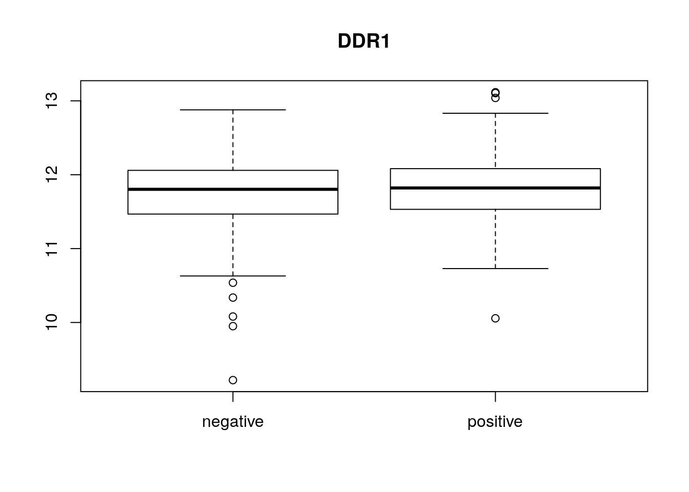

limma pipeline

design <- model.matrix(~er, data = pData(eset))
head(design, 2)

      (Intercept) erpositive
VDX_3           1          0
VDX_5           1          1

colSums(design)

(Intercept)  erpositive 
        344         209

table(pData(eset)[, "er"])


negative positive 
     135      209

library(limma)


Attaching package: 'limma'

The following object is masked from 'package:BiocGenerics':

    plotMA

fit <- lmFit(eset, design)
head(fit$coefficients, 3)

          (Intercept)  erpositive
1007_s_at   11.725148  0.09878782
1053_at      8.126934 -0.54673000
117_at       7.972049 -0.17342654

fit <- eBayes(fit)
head(fit$t, 3)

          (Intercept) erpositive
1007_s_at    276.8043   1.817824
1053_at      122.5899  -6.428278
117_at       164.0240  -2.781294

results <- decideTests(fit[, "erpositive"])
summary(results)

   erpositive
-1       6276
0       11003
1        5004

group-means

design <- model.matrix(~0 + er, data = pData(eset))
head(design)

      ernegative erpositive
VDX_3          1          0
VDX_5          0          1
VDX_6          1          0
VDX_7          1          0
VDX_8          1          0
VDX_9          0          1

colSums(design)

ernegative erpositive 
       135        209

library(limma)
cm <- makeContrasts(status = erpositive - ernegative,
                    levels = design)
cm

            Contrasts
Levels       status
  ernegative     -1
  erpositive      1

fit <- lmFit(eset, design)
head(fit$coefficients)

          ernegative erpositive
1007_s_at  11.725148  11.823936
1053_at     8.126934   7.580204
117_at      7.972049   7.798623
121_at     10.168975  10.086393
1255_g_at   5.903189   5.729195
1294_at     9.166436   9.390949

fit2 <- contrasts.fit(fit, contrasts = cm)
head(fit2$coefficients)

           Contrasts
                 status
  1007_s_at  0.09878782
  1053_at   -0.54673000
  117_at    -0.17342654
  121_at    -0.08258267
  1255_g_at -0.17399402
  1294_at    0.22451339

fit2 <- eBayes(fit2)
results <- decideTests(fit2)
summary(results)

topTable(fit2)

              symbol entrez   chrom    logFC   AveExpr        t
205225_at       ESR1   2099  6q25.1 3.762901 11.377735 22.68392
209603_at      GATA3   2625   10p15 3.052348  9.941990 18.98154
209604_s_at    GATA3   2625   10p15 2.431309 13.185334 17.59968
212956_at     TBC1D9  23158 4q31.21 2.157435 11.702942 17.48711
202088_at    SLC39A6  25800 18q12.2 1.719680 13.119496 17.30104
212496_s_at    KDM4B  23030 19p13.3 1.459843 10.703942 16.85070
215867_x_at     CA12    771   15q22 2.246120 11.450485 16.79123
209602_s_at    GATA3   2625   10p15 2.921505  9.547850 16.43202
212195_at      IL6ST   3572    5q11 1.381778 11.737839 16.31864
218195_at   C6orf211  79624  6q25.1 1.738740  9.479901 16.27378
                 P.Value    adj.P.Val         B
205225_at   2.001001e-70 4.458832e-66 149.19866
209603_at   1.486522e-55 1.656209e-51 115.46414
209604_s_at 5.839050e-50 4.337052e-46 102.75707
212956_at   1.665700e-49 9.279201e-46 101.72268
202088_at   9.412084e-49 4.194589e-45 100.01376
212496_s_at 6.188671e-47 2.298369e-43  95.88265
215867_x_at 1.074845e-46 3.421537e-43  95.33780
209602_s_at 3.004184e-45 8.367780e-42  92.05058
212195_at   8.581176e-45 2.124604e-41  91.01458
218195_at   1.299472e-44 2.895613e-41  90.60496

Visualize results

For Ch3 L2 plotMDS/removeBatchEffect

stats <- topTable(fit2, number = nrow(fit2), sort.by = "none")
dim(stats)

[1] 22283     9

hist(runif(10000))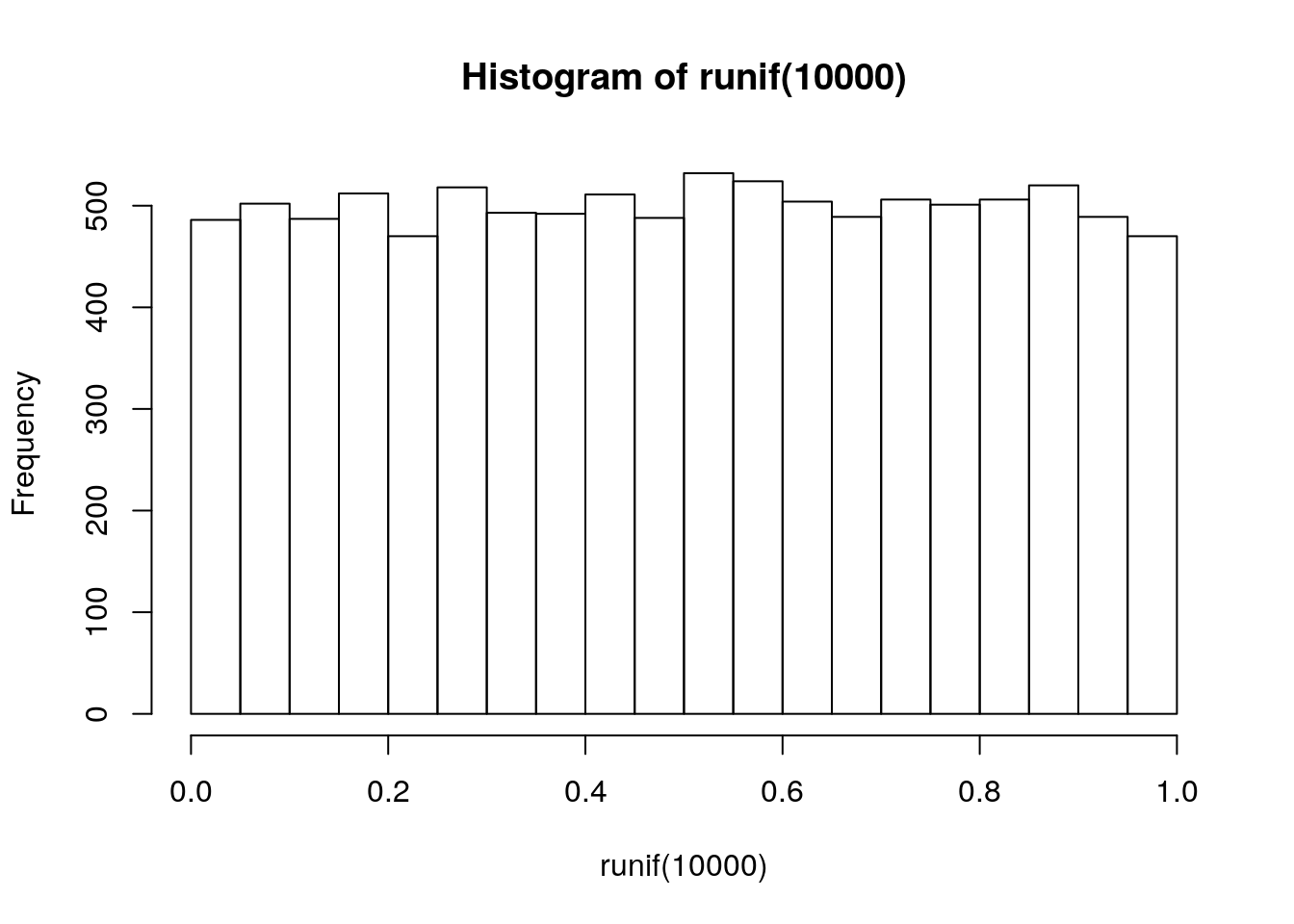

hist(stats[, "P.Value"])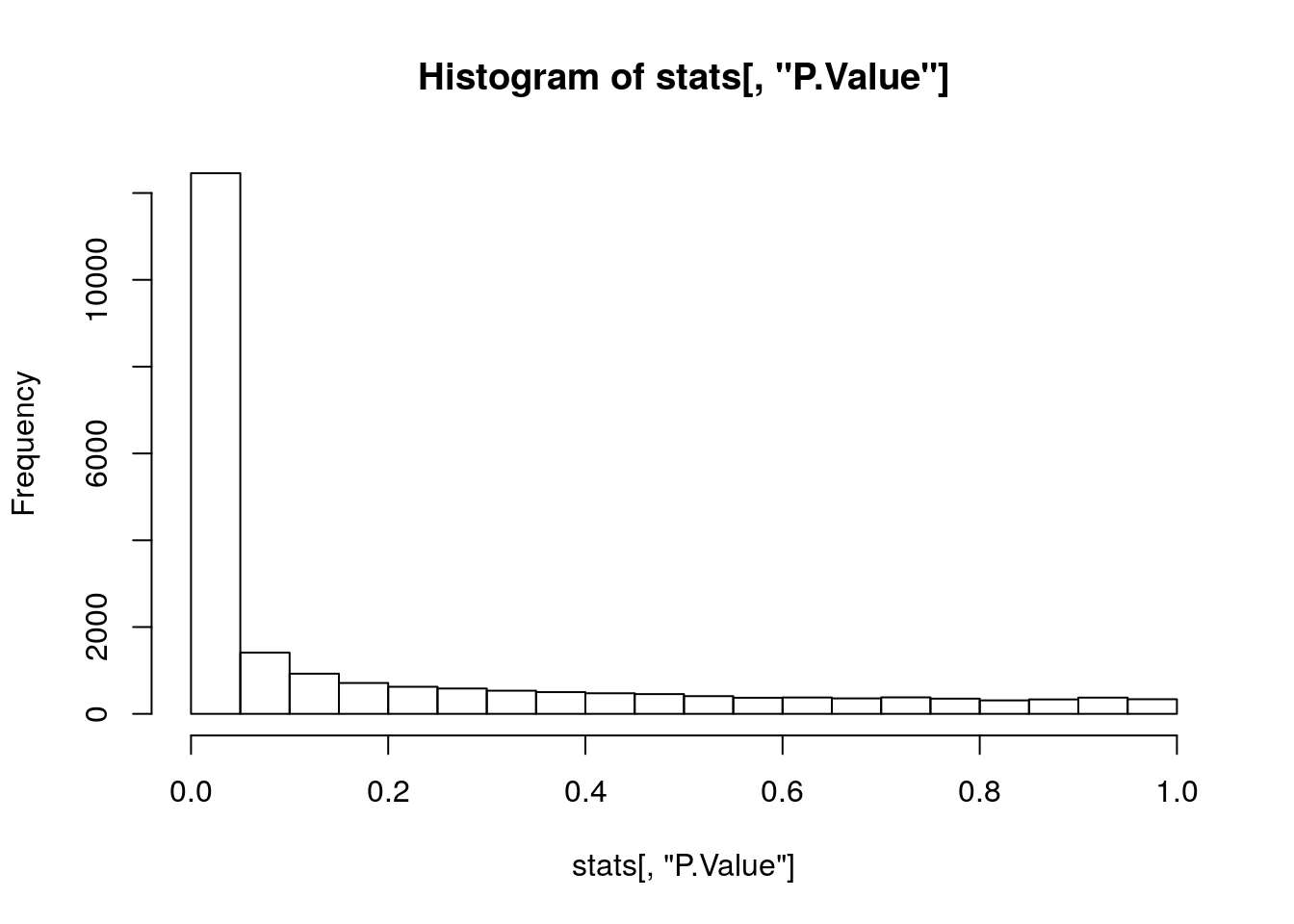

volcanoplot(fit2, highlight = 5, names = fit2$genes[, "symbol"])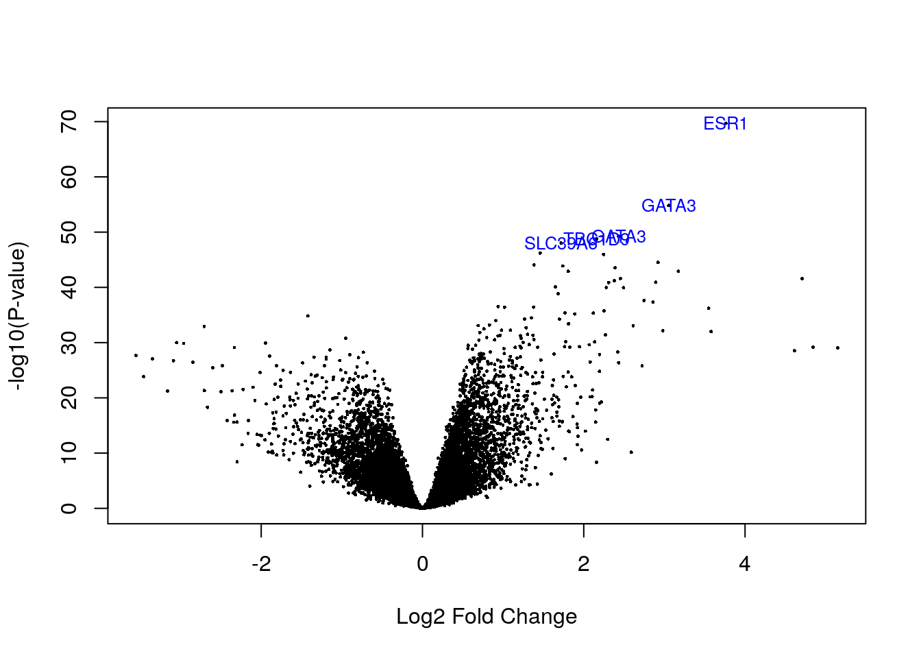

Enrichment

topTable(fit2, number = 3)

            symbol entrez  chrom    logFC  AveExpr        t      P.Value
205225_at     ESR1   2099 6q25.1 3.762901 11.37774 22.68392 2.001001e-70
209603_at    GATA3   2625  10p15 3.052348  9.94199 18.98154 1.486522e-55
209604_s_at  GATA3   2625  10p15 2.431309 13.18533 17.59968 5.839050e-50
               adj.P.Val        B
205225_at   4.458832e-66 149.1987
209603_at   1.656209e-51 115.4641
209604_s_at 4.337052e-46 102.7571

# 1000 genes (10% in gene set), 100 are DE (10% in gene set)
fisher.test(matrix(c(10, 100, 90, 900), nrow = 2))


    Fisher's Exact Test for Count Data

data:  matrix(c(10, 100, 90, 900), nrow = 2)
p-value = 1
alternative hypothesis: true odds ratio is not equal to 1
95 percent confidence interval:
 0.4490765 2.0076377
sample estimates:
odds ratio 
         1

# 1000 genes (10% in gene set), 100 are DE (30% in gene set)
fisher.test(matrix(c(30, 100, 70, 900), nrow = 2))


    Fisher's Exact Test for Count Data

data:  matrix(c(30, 100, 70, 900), nrow = 2)
p-value = 1.88e-07
alternative hypothesis: true odds ratio is not equal to 1
95 percent confidence interval:
 2.306911 6.320992
sample estimates:
odds ratio 
  3.850476

head(fit2$genes, 3)

          symbol entrez   chrom
1007_s_at   DDR1    780  6p21.3
1053_at     RFC2   5982 7q11.23
117_at     HSPA6   3310    1q23

entrez <- fit2$genes[, "entrez"]


enrich_kegg <- kegga(fit2, geneid = entrez, species = "Hs")
topKEGG(enrich_kegg, number = 4)

                          Pathway    N  Up Down         P.Up       P.Down
path:hsa04110          Cell cycle  115  30   82 6.188398e-01 5.027045e-12
path:hsa05166    HTLV-I infection  233  55  135 8.956123e-01 9.165684e-09
path:hsa01100  Metabolic pathways 1033 350  373 3.109042e-08 9.969222e-01
path:hsa04218 Cellular senescence  145  32   88 9.269545e-01 2.249635e-07

enrich_go <- goana(fit2, geneid = entrez, species = "Hs")
topGO(enrich_go, ontology = "BP", number = 3)

                             Term Ont    N  Up Down P.Up       P.Down
GO:0002376  immune system process  BP 2235 509 1055    1 8.273520e-38
GO:0006955        immune response  BP 1562 316  772    1 9.287064e-35
GO:0045087 innate immune response  BP  673 114  361    1 1.197071e-23

Session information

sessionInfo()

R version 3.4.4 (2018-03-15)
Platform: x86_64-pc-linux-gnu (64-bit)
Running under: Ubuntu 18.04.1 LTS

Matrix products: default
BLAS: /usr/lib/x86_64-linux-gnu/blas/libblas.so.3.7.1
LAPACK: /usr/lib/x86_64-linux-gnu/lapack/liblapack.so.3.7.1

locale:
 [1] LC_CTYPE=en_US.UTF-8       LC_NUMERIC=C              
 [3] LC_TIME=en_US.UTF-8        LC_COLLATE=en_US.UTF-8    
 [5] LC_MONETARY=en_US.UTF-8    LC_MESSAGES=en_US.UTF-8   
 [7] LC_PAPER=en_US.UTF-8       LC_NAME=C                 
 [9] LC_ADDRESS=C               LC_TELEPHONE=C            
[11] LC_MEASUREMENT=en_US.UTF-8 LC_IDENTIFICATION=C       

attached base packages:
[1] parallel  stats     graphics  grDevices utils     datasets  methods  
[8] base     

other attached packages:
[1] limma_3.32.2           breastCancerVDX_1.14.0 Biobase_2.36.2        
[4] BiocGenerics_0.22.1   

loaded via a namespace (and not attached):
 [1] Rcpp_0.12.17         AnnotationDbi_1.38.2 knitr_1.20          
 [4] whisker_0.3-2        magrittr_1.5         workflowr_1.1.1.9000
 [7] IRanges_2.10.5       bit_1.1-12           org.Hs.eg.db_3.4.1  
[10] blob_1.1.1           stringr_1.3.0        tools_3.4.4         
[13] R.oo_1.22.0          DBI_1.0.0            git2r_0.21.0        
[16] htmltools_0.3.6      bit64_0.9-7          yaml_2.1.19         
[19] rprojroot_1.3-2      digest_0.6.15        S4Vectors_0.14.7    
[22] R.utils_2.6.0        memoise_1.1.0        RSQLite_2.1.0       
[25] evaluate_0.10.1      rmarkdown_1.9        stringi_1.2.2       
[28] compiler_3.4.4       GO.db_3.4.1          backports_1.1.2-9000
[31] R.methodsS3_1.7.1    stats4_3.4.4         pkgconfig_2.0.1

This reproducible R Markdown analysis was created with workflowr 1.1.1.9000