Gene filtering
Joyce Hsiao
Last updated: 2017-12-21
Code version: 62c60ea
Summary
I performed gene filtering based on the criterion set forth in our previous paper.
- Remove mitochrodrial genes: filter out mitochrondrial genes verified and listed in MitoCarta.
Results:Found 1,150 genes previously quantified in MitoCarta inventory.
Output: gene annotation saved in ../output/gene-filtering.Rmd/mito-genes-info.csv
\(~\)
- Remove outlier genes: molecule counts > 4,096 in any sample (x is the theoretical maximum of UMI count for 6-bp UMI)
Results There’s one, and turns out this over-expressed gene is one of the mitochrondrial genes.
Output: gene annotation saved in ../output/gene-filtering.Rmd/over-expressed-genes-info.csv
\(~\)
- Remove lowly expressed genes: Lowly-expressed genes := gene mean < 2 CPM.
Results: * Of 20,421 genes, 7,864 genes are classifed as lowly-expressed. Of these, 34 are ERCC control genes and 7,830 are endogenoeus genes.
Output: gene annotation saved in ../output/gene-filtering.Rmd/lowly-expressed-genes-info.csv
Finally, filtered eset (eset_filtered) and cpm normalized count (cpm_filtered) are saved in ../output/gene-filtering.Rmd/eset-filterd.rdata.
\(~\)
Import data
Combine eSet objects.
library(knitr)
library(Biobase)
#library(gdata)
library(testit)
library(cowplot)
library(biomaRt)
library(knitr)
library(data.table)

source("../code/pca.R")
eset <- readRDS("../output_tmp/eset.rds")
Filter out low-quality single cell samples.
pdata_filter <- pData(eset)[pData(eset)$filter_all == TRUE,]
count_filter <- exprs(eset[,pData(eset)$filter_all == TRUE])
dim(count_filter)
[1] 20421 1025\(~\)
Mitochrondrial genes
Found 1,150 genes previously quantified in MitoCarta inventory.
human_mito <- gdata::read.xls("../data/Human.MitoCarta2.0.xls",
                   sheet = 2, header = TRUE, stringsAsFactors=FALSE)
human_mito_ensembl <- human_mito$EnsemblGeneID

which_mito <- which(rownames(count_filter) %in% human_mito_ensembl)
which_mito_genes <- rownames(count_filter)[which_mito]

length(which_mito)
[1] 1150Get mito gene info via biomaRt.
# do biomart to verfiy these genes
ensembl <- useMart(host = "grch37.ensembl.org",
                   biomart = "ENSEMBL_MART_ENSEMBL",
                   dataset = "hsapiens_gene_ensembl")

mito_genes_info <- getBM(
  attributes = c("ensembl_gene_id", "chromosome_name",
                 "external_gene_name", "transcript_count",
                 "description"),
  filters = "ensembl_gene_id",
  values = which_mito_genes[grep("ENSG", which_mito_genes)],
  mart = ensembl)


fwrite(mito_genes_info,
       file = "../output/gene-filtering.Rmd/mito-genes-info.csv")
\(~\)
Over-expressed genes
There’s one, and turns out this over-expressed gene is one of the mitochrondrial genes.
which_over_expressed <- which(apply(count_filter, 1, function(x) any(x>(4^6)) ))
over_expressed_genes <- rownames(count_filter)[which_over_expressed]
over_expressed_genes %in% human_mito_ensembl
[1] TRUEover_expressed_genes[1] "ENSG00000198886"Get over-expressed gene info via biomaRt.
over_expressed_genes_info <- getBM(
  attributes = c("ensembl_gene_id", "chromosome_name",
                 "external_gene_name", "transcript_count",
                 "description"),
  filters = "ensembl_gene_id",
  values = over_expressed_genes,
  mart = ensembl)

fwrite(over_expressed_genes_info,
       file = "../output/gene-filtering.Rmd/over-expressed-genes-info.csv")
\(~\)
Filter out lowly-expressed genes
- Of 20,421 genes, 7,864 genes are classifed as lowly-expressed. Of these, 34 are ERCC control genes and 7,830 are endogenoeus genes.
Compute CPM
cpm <- t(t(count_filter)/colSums(count_filter))*(10^6)Lowly-expressed genes := gene mean < 2 CPM
which_lowly_expressed <- which(rowMeans(cpm) < 2)
length(which_lowly_expressed)
[1] 7864which_lowly_expressed_genes <- rownames(cpm)[which_lowly_expressed]
length(grep("ERCC", which_lowly_expressed_genes))[1] 34length(grep("ENSG", which_lowly_expressed_genes))[1] 7830Get gene info via biomaRt.
lowly_expressed_genes_info <- getBM(
  attributes = c("ensembl_gene_id", "chromosome_name",
                 "external_gene_name", "transcript_count",
                 "description"),
  filters = "ensembl_gene_id",
  values = which_lowly_expressed_genes[grep("ENSG", which_lowly_expressed_genes)],
  mart = ensembl)

fwrite(lowly_expressed_genes_info,
       file = "../output/gene-filtering.Rmd/lowly-expressed-genes-info.csv")
\(~\)
Combine filters
Including 16,460 genes.
gene_filter <- unique(c(which_lowly_expressed, which_mito, which_over_expressed))

genes_to_include <- setdiff(1:nrow(count_filter), gene_filter)
length(genes_to_include)
[1] 11489\(~\)
Make filtered data
cpm_filtered <- cpm[genes_to_include, ]

eset_filtered <- eset[genes_to_include, pData(eset)$filter_all==TRUE]
eset_filtered
ExpressionSet (storageMode: lockedEnvironment)
assayData: 11489 features, 1025 samples
element names: exprs
protocolData: none
phenoData
sampleNames: 20170905-A01 20170905-A02 ... 20170924-H12 (1025
total)
varLabels: experiment well ... filter_all (43 total)
varMetadata: labelDescription
featureData
featureNames: EGFP ENSG00000000003 ... mCherry (11489 total)
fvarLabels: chr start ... source (6 total)
fvarMetadata: labelDescription
experimentData: use 'experimentData(object)'
Annotation: save(cpm_filtered, eset_filtered,
file = "../output/gene-filtering.Rmd/eset-filtered.rdata")\(~\)
Compute log2 CPM
Import data post sample and gene filtering.
load(file="../output/gene-filtering.Rmd/eset-filtered.rdata")Compute log2 CPM based on the library size before filtering.
log2cpm <- log2(cpm_filtered+1)\(~\)
PCA
pca_log2cpm <- run_pca(log2cpm)

pdata <- pData(eset_filtered)
pdata$experiment <- as.factor(pdata$experiment)

plot_grid(
  plot_pca(x=pca_log2cpm$PCs, explained=pca_log2cpm$explained,
         metadata=pdata, color="chip_id"),
  plot_pca(x=pca_log2cpm$PCs, explained=pca_log2cpm$explained,
         metadata=pdata, color="experiment"),
  ncol=2)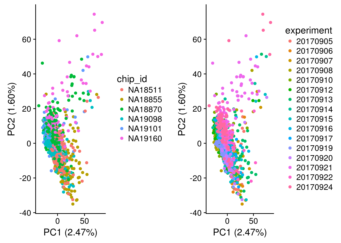
\(~\)
Session information
R version 3.4.1 (2017-06-30)
Platform: x86_64-pc-linux-gnu (64-bit)
Running under: Scientific Linux 7.2 (Nitrogen)

Matrix products: default
BLAS: /home/joycehsiao/miniconda3/envs/fucci-seq/lib/R/lib/libRblas.so
LAPACK: /home/joycehsiao/miniconda3/envs/fucci-seq/lib/R/lib/libRlapack.so

locale:
 [1] LC_CTYPE=en_US.UTF-8       LC_NUMERIC=C
 [3] LC_TIME=en_US.UTF-8        LC_COLLATE=en_US.UTF-8
 [5] LC_MONETARY=en_US.UTF-8    LC_MESSAGES=en_US.UTF-8
 [7] LC_PAPER=en_US.UTF-8       LC_NAME=C
 [9] LC_ADDRESS=C               LC_TELEPHONE=C
[11] LC_MEASUREMENT=en_US.UTF-8 LC_IDENTIFICATION=C

attached base packages:
[1] parallel  stats     graphics  grDevices utils     datasets  methods
[8] base

other attached packages:
[1] data.table_1.10.4   biomaRt_2.34.0      cowplot_0.8.0
[4] ggplot2_2.2.1       testit_0.7          Biobase_2.38.0
[7] BiocGenerics_0.24.0 knitr_1.17

loaded via a namespace (and not attached):
 [1] Rcpp_0.12.14         compiler_3.4.1       git2r_0.19.0
 [4] plyr_1.8.4           prettyunits_1.0.2    progress_1.1.2
 [7] bitops_1.0-6         tools_3.4.1          digest_0.6.12
[10] bit_1.1-12           evaluate_0.10.1      RSQLite_2.0
[13] memoise_1.1.0        tibble_1.3.3         gtable_0.2.0
[16] rlang_0.1.4.9000     DBI_0.6-1            yaml_2.1.16
[19] stringr_1.2.0        gtools_3.5.0         IRanges_2.12.0
[22] S4Vectors_0.16.0     stats4_3.4.1         rprojroot_1.2
[25] bit64_0.9-5          grid_3.4.1           R6_2.2.2
[28] AnnotationDbi_1.40.0 XML_3.98-1.6         rmarkdown_1.8
[31] gdata_2.18.0         blob_1.1.0           magrittr_1.5
[34] backports_1.0.5      scales_0.4.1         htmltools_0.3.6
[37] assertthat_0.2.0     colorspace_1.3-2     labeling_0.3
[40] stringi_1.1.2        RCurl_1.95-4.8       lazyeval_0.2.0
[43] munsell_0.4.3
This R Markdown site was created with workflowr