Batch effect in RNA-seq data
Joyce Hsiao
Last updated: 2018-02-14
Code version: 3267559
Introduction/summary
The experimental design for our study is commonly known as “incomplete block design”. The individuals are grouped into combinations of two, and no two individuals appear in the same combination twice. In our study, combination refers to C1 plates, so the combination of cell lines on each C1 plate is thereofre unique.
In notations,
\(N\): number of individuals \(k\): combination size (in our case, each combinatino is a plate) \(B\): number of plates \(r_i\): number of replicates for individual \(i\) in the entire design
For now assume \(r_i=r\) for all individuals. Then, in our design each individual replicate can pair up with \(N-1/k-1\) possible number of individuals. And since the pairs consist of unique individuals, so there can be \(N-1/k-1\) possible number of replicates for each individual. We have \(N=6, k=2\) which gives 5 replicates per individual cell line.
Our design is in principle balanced, i.e., each pair of individuals occurs together one time in the study. But at the end of the experiment, we collected an additional C1 plate on the first pair of individuals processed. This gives us a total of 16 plates (pairs or blocks).
I performed analysis of variance for intensity data using the following model
\[ y_{ij} = \mu + \tau_i + \beta_j + \epsilon_{ij} \] where \(i = 1,2,..., N\) and \(j = 1,2,..., B\). The parameters are estimated under sum-to-zero constraints \(\sum \tau_i = 0\) and \(\sum \beta_j = 0\).
Note that in this model 1) not all \(y_{ij}\) exists due to the incompleteness of the design, 2) the effects of individual and block are nonorthogonal, 3) the effects are additive due to the block design.
We analyzed data normalized to log2CPM and used the ibd package for each gene to
Estimate prop of variance explained by individual and plate.
Estimate mean effect from each plate and remove this estimated effect from each gene
TO DO: apply shrinkage to the estimated mean effect??
Load data
\(~\)
library(data.table)
library(dplyr)
library(ggplot2)
library(cowplot)
library(wesanderson)
library(RColorBrewer)
library(Biobase)
library(scales)
library(stringr)
library(heatmap3)

# note that ibd is not in the fucci-seq conda environment
library(ibd)
Read in filtered data.
df <- readRDS(file="../data/eset-filtered.rds")
pdata <- pData(df)
fdata <- fData(df)
counts <- exprs(df)
library size variation
boxplot(pdata$molecules~pdata$experiment,
        xlab = "Plate", ylab = "log10 library size")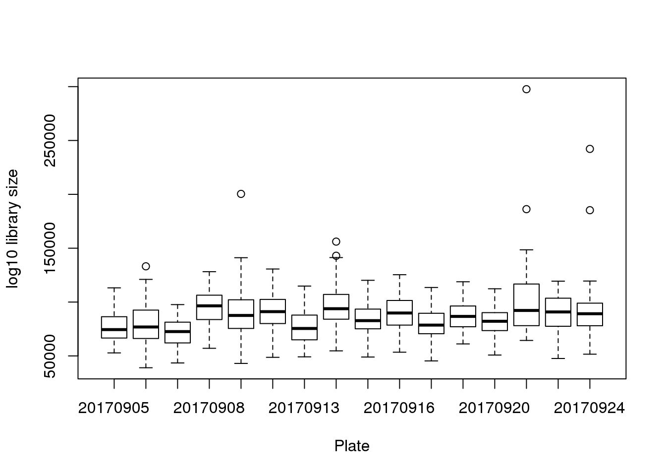
boxplot(pdata$molecules~pdata$chip_id,
        xlab = "Plate", ylab = "log10 library size")
counts to log2cpm
log2cpm <- t(log2(1+(10^6)*(t(counts)/pdata$molecules)))save log2cpm
saveRDS(log2cpm, file = "../output/seqdata-batch-correction.Rmd/log2cpm.rds")convert sample well to two labels: rows and columns
pdata$well_row <- str_sub(pdata$well,1,1)
pdata$well_col <- str_sub(pdata$well,2,3)
batch variation
total molecules significant differs between individuals and batch
ibd_mol <- aov.ibd(log10(molecules)~factor(chip_id)+factor(experiment),data=pdata)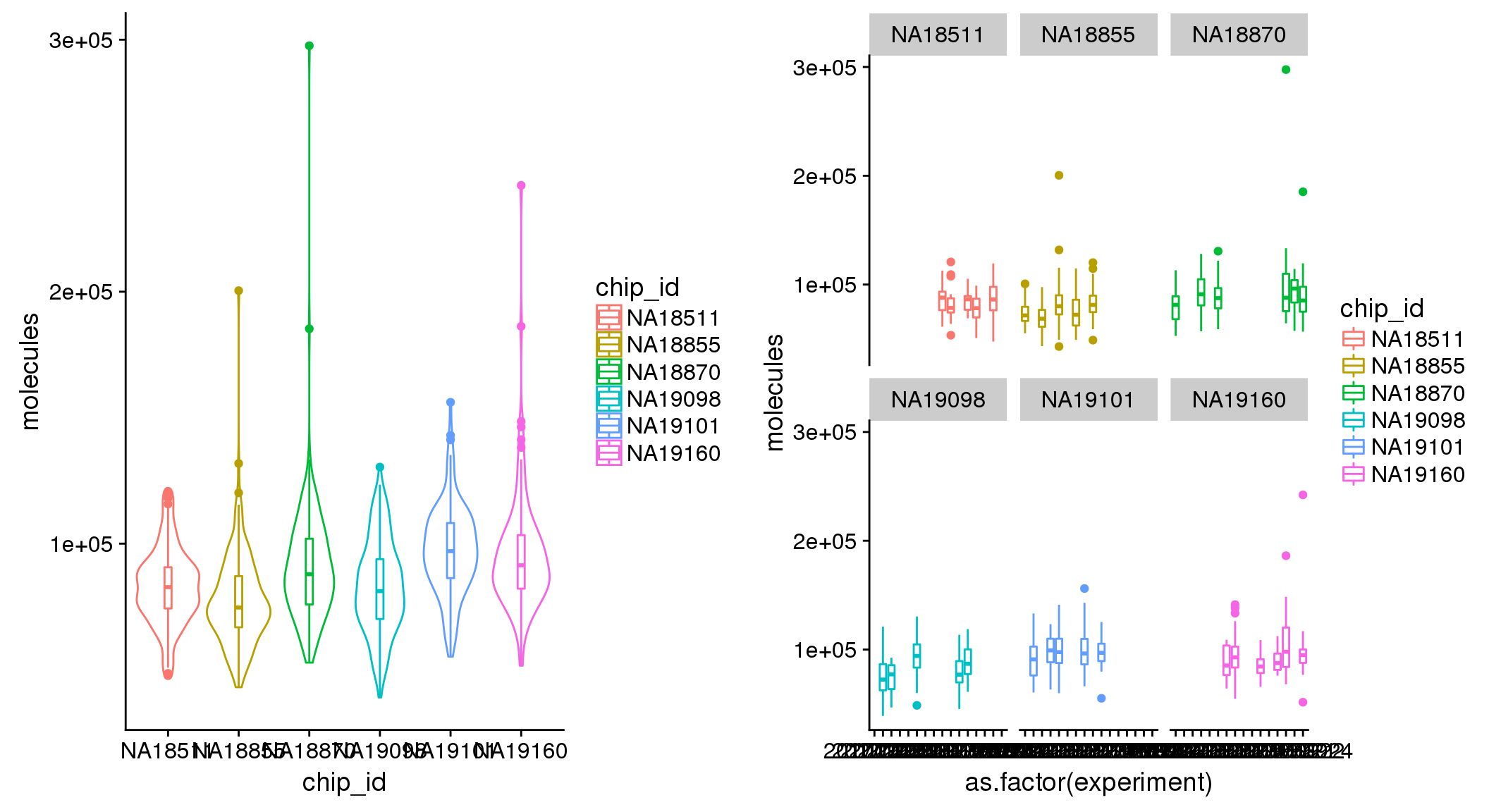
per gene log2cpm anova
ibd_genes <- lapply(1:nrow(log2cpm), function(i) {
  aov.ibd(log2cpm[i,]~factor(chip_id)+factor(experiment),data=pdata)
})

saveRDS(ibd_genes, file = "../output/seqdata-batch-correction.Rmd/ibd-genes.rds")
This seems to suggest that there’s no relationship between proportion of variance explained by indivdiual and by plate. Note that in these per-gene analysis, intercept explains a significant large portion of the variance, suggesting an overall large deviation of sample log2cpm from the mean.
ibd_genes <- readRDS("../output/seqdata-batch-correction.Rmd/ibd-genes.rds")
ind_varprop <- sapply(ibd_genes, function(x)  x[[1]]$`Sum Sq`[2]/sum(x[[1]]$`Sum Sq`))
plate_varprop <- sapply(ibd_genes, function(x)  x[[1]]$`Sum Sq`[3]/sum(x[[1]]$`Sum Sq`))


plot(log10(ind_varprop), log10(plate_varprop), xlim=c(-4,0), ylim=c(-4,0),
     pch=16, cex=.7)
Estimate plate effect
# make contrast matrix
n_plates <- uniqueN(pdata$experiment)
contrast_plates <- matrix(-1, nrow=n_plates, ncol=n_plates)
diag(contrast_plates) <- n_plates-1

log2cpm.adjust <- log2cpm
for (i in 1:nrow(log2cpm)) {
  ibd_exp <- aov.ibd(log2cpm[i,]~factor(chip_id)+factor(experiment),
          data=pdata, spec="experiment", contrast=contrast_plates)
  ibd_est <- ibd_exp$LSMEANS

  exps <- unique(pdata$experiment)
  for (j in 1:uniqueN(exps)) {
    exp <- exps[j]
    ii_exp <- which(pdata$experiment == exp)
    est_exp <- ibd_est$lsmean[which(ibd_est$experiment==exp)]
    log2cpm.adjust[i,ii_exp] <- log2cpm[i,ii_exp] - est_exp
  }
  }

saveRDS(log2cpm.adjust, file = "../output/seqdata-batch-correction.Rmd/log2cpm.adjust.rds")
log2cpm.adjust <- readRDS("../output/seqdata-batch-correction.Rmd/log2cpm.adjust.rds")PCA after adjustment. Somehow now well has significant contribution to PC1…
pca_log2cpm_adjust <- prcomp(t(log2cpm.adjust), center = TRUE)

covariates <- pdata %>% dplyr::select(experiment, well_row, well_col, chip_id,
                                                     concentration, raw:unmapped,
                                                     starts_with("detect"),  molecules)
## look at the first 6 PCs
pcs <- pca_log2cpm_adjust$x[, 1:6]

## generate the data
get_r2 <- function(x, y) {
  stopifnot(length(x) == length(y))
  model <- lm(y ~ x)
  stats <- summary(model)
  return(stats$adj.r.squared)
}

r2 <- matrix(NA, nrow = ncol(covariates), ncol = ncol(pcs),
             dimnames = list(colnames(covariates), colnames(pcs)))
for (cov in colnames(covariates)) {
  for (pc in colnames(pcs)) {
    r2[cov, pc] <- get_r2(covariates[, cov], pcs[, pc])
  }
}

## plot heatmap
heatmap3(r2, cexRow=1, cexCol=1, margins=c(8,8), scale = "none",
         col=brewer.pal(9,"YlGn"), showColDendro = F, Colv = NA,
         ylab="technical factor", main = "Batch-corrected data")
PCA before adjustment.
pca_log2cpm <- prcomp(t(log2cpm), center = TRUE)

covariates <- pdata %>% dplyr::select(experiment, well_row, well_col, chip_id,
                                                     concentration, raw:unmapped,
                                                     starts_with("detect"),  molecules)
## look at the first 6 PCs
pcs <- pca_log2cpm$x[, 1:6]

## generate the data
get_r2 <- function(x, y) {
  stopifnot(length(x) == length(y))
  model <- lm(y ~ x)
  stats <- summary(model)
  return(stats$adj.r.squared)
}

r2 <- matrix(NA, nrow = ncol(covariates), ncol = ncol(pcs),
             dimnames = list(colnames(covariates), colnames(pcs)))
for (cov in colnames(covariates)) {
  for (pc in colnames(pcs)) {
    r2[cov, pc] <- get_r2(covariates[, cov], pcs[, pc])
  }
}

## plot heatmap
heatmap3(r2, cexRow=1, cexCol=1, margins=c(8,8), scale = "none",
         col=brewer.pal(9,"YlGn"), showColDendro = F, Colv = NA,
         ylab="technical factor", main = "Before batch correction")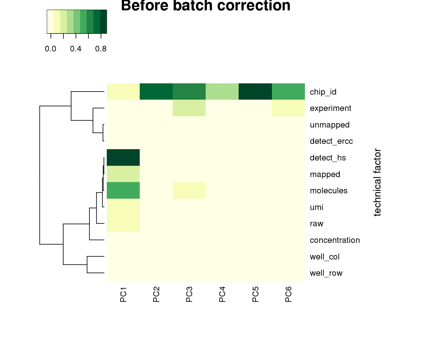
Session information
R version 3.4.1 (2017-06-30)
Platform: x86_64-redhat-linux-gnu (64-bit)
Running under: Scientific Linux 7.2 (Nitrogen)

Matrix products: default
BLAS/LAPACK: /usr/lib64/R/lib/libRblas.so

locale:
 [1] LC_CTYPE=en_US.UTF-8       LC_NUMERIC=C
 [3] LC_TIME=en_US.UTF-8        LC_COLLATE=en_US.UTF-8
 [5] LC_MONETARY=en_US.UTF-8    LC_MESSAGES=en_US.UTF-8
 [7] LC_PAPER=en_US.UTF-8       LC_NAME=C
 [9] LC_ADDRESS=C               LC_TELEPHONE=C
[11] LC_MEASUREMENT=en_US.UTF-8 LC_IDENTIFICATION=C

attached base packages:
[1] parallel  stats     graphics  grDevices utils     datasets  methods
[8] base

other attached packages:
 [1] ibd_1.2             multcompView_0.1-7  lsmeans_2.27-61
 [4] car_2.1-6           MASS_7.3-47         lpSolve_5.6.13
 [7] heatmap3_1.1.1      stringr_1.2.0       scales_0.5.0
[10] Biobase_2.38.0      BiocGenerics_0.24.0 RColorBrewer_1.1-2
[13] wesanderson_0.3.4   cowplot_0.9.2       ggplot2_2.2.1
[16] dplyr_0.7.4         data.table_1.10.4-3

loaded via a namespace (and not attached):
 [1] fastcluster_1.1.24 zoo_1.8-1          splines_3.4.1
 [4] lattice_0.20-35    colorspace_1.3-2   htmltools_0.3.6
 [7] yaml_2.1.16        mgcv_1.8-17        survival_2.41-3
[10] rlang_0.1.6        pillar_1.1.0       nloptr_1.0.4
[13] glue_1.2.0         bindrcpp_0.2       multcomp_1.4-8
[16] bindr_0.1          plyr_1.8.4         MatrixModels_0.4-1
[19] munsell_0.4.3      gtable_0.2.0       mvtnorm_1.0-7
[22] coda_0.19-1        codetools_0.2-15   evaluate_0.10.1
[25] labeling_0.3       knitr_1.19         SparseM_1.77
[28] quantreg_5.35      pbkrtest_0.4-7     TH.data_1.0-8
[31] Rcpp_0.12.15       xtable_1.8-2       backports_1.1.2
[34] lme4_1.1-15        digest_0.6.15      stringi_1.1.6
[37] grid_3.4.1         rprojroot_1.3-2    tools_3.4.1
[40] sandwich_2.4-0     magrittr_1.5       lazyeval_0.2.1
[43] tibble_1.4.2       pkgconfig_2.0.1    Matrix_1.2-10
[46] estimability_1.2   assertthat_0.2.0   minqa_1.2.4
[49] rmarkdown_1.8      R6_2.2.2           nnet_7.3-12
[52] nlme_3.1-131       git2r_0.21.0       compiler_3.4.1
This R Markdown site was created with workflowr