Select genes indicative of cell cycle state
Joyce Hsiao
Last updated: 2018-04-10
Code version: b8f2627
Estimate cell time
library(Biobase)
# load gene expression
df <- readRDS(file="../data/eset-final.rds")
pdata <- pData(df)
fdata <- fData(df)

# select endogeneous genes
counts <- exprs(df)[grep("ENSG", rownames(df)), ]

log2cpm.all <- t(log2(1+(10^6)*(t(counts)/pdata$molecules)))


pdata.adj <- readRDS("../output/images-normalize-anova.Rmd/pdata.adj.rds")

macosko <- readRDS("../data/cellcycle-genes-previous-studies/rds/macosko-2015.rds")

pc.fucci <- prcomp(subset(pdata.adj,
                          select=c("rfp.median.log10sum.adjust",
                                   "gfp.median.log10sum.adjust")),
                   center = T, scale. = T)
Theta.cart <- pc.fucci$x
library(circular)
Theta.fucci <- coord2rad(Theta.cart)
Theta.fucci <- 2*pi - Theta.fucci
Cluster cell times to move the origin of the cell times
# cluster cell time
library(movMF)
clust.res <- lapply(2:5, function(k) {
  movMF(Theta.cart, k=k, nruns = 100, kappa = list(common = TRUE))
})
k.list <- sapply(clust.res, function(x) length(x$theta) + length(x$alpha) + 1)
bic <- sapply(1:length(clust.res), function(i) {
  x <- clust.res[[i]]
  k <- k.list[i]
  n <- nrow(Theta.cart)
  -2*x$L + k *(log(n) - log(2*pi)) })
plot(bic)
labs <- predict(clust.res[[2]])

saveRDS(labs, file = "../output/images-time-eval.Rmd/labs.rds")
labs <- readRDS(file = "../output/images-time-eval.Rmd/labs.rds")
summary(as.numeric(Theta.fucci)[labs==1]) Min. 1st Qu. Median Mean 3rd Qu. Max.
1.277 1.978 2.392 2.336 2.692 3.525 summary(as.numeric(Theta.fucci)[labs==2]) Min. 1st Qu. Median Mean 3rd Qu. Max.
3.579 4.348 4.689 4.675 5.007 5.809 summary(as.numeric(Theta.fucci)[labs==3]) Min. 1st Qu. Median Mean 3rd Qu. Max.
0.004806 0.434017 0.874891 2.095213 5.830072 6.278717 # move the origin to 1.27
Theta.fucci.new <- vector("numeric", length(Theta.fucci))
cutoff <- min(Theta.fucci[labs==1])
Theta.fucci.new[Theta.fucci>=cutoff] <- Theta.fucci[Theta.fucci>=cutoff] - cutoff
Theta.fucci.new[Theta.fucci<cutoff] <- Theta.fucci[Theta.fucci<cutoff] - cutoff + 2*piTry plotting for one gene
macosko[macosko$hgnc == "CDK1",] hgnc phase ensembl
113 CDK1 G2 ENSG00000170312cdk1 <- log2cpm.all[rownames(log2cpm.all)=="ENSG00000170312",]
plot(x=Theta.fucci.new, y = cdk1)
points(y=cdk1[labs==1], x=as.numeric(Theta.fucci.new)[labs==1], pch=16, cex=.7, col = "red")
points(y=cdk1[labs==2], x=as.numeric(Theta.fucci.new)[labs==2], pch=16, cex=.7, col = "forestgreen")
points(y=cdk1[labs==3], x=as.numeric(Theta.fucci.new)[labs==3], pch=16, cex=.7, col = "blue")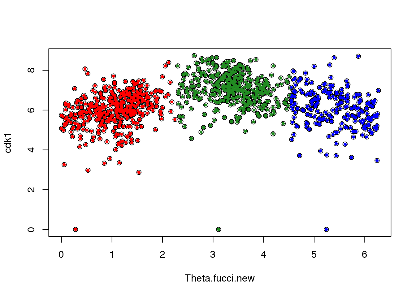
Results
par(mfrow=c(2,2))
ylims <- with(pdata.adj, range(c(dapi.median.log10sum.adjust,
                                 gfp.median.log10sum.adjust,
                                 rfp.median.log10sum.adjust)))
plot(as.numeric(Theta.fucci.new), pdata.adj$dapi.median.log10sum.adjust, col = "blue",
     ylab= "adjusted intensity values",
     ylim = ylims, main = "DAPI intensity values",
     xlab ="Estimated cell time")
plot(as.numeric(Theta.fucci.new), pdata.adj$gfp.median.log10sum.adjust, col = "forestgreen",
     ylab= "adjusted intensity values",
     ylim = ylims, main = "GFP and RFP intensity values",
     xlab ="Estimated cell time")
points(as.numeric(Theta.fucci.new), pdata.adj$rfp.median.log10sum.adjust, col = "red")
plot(as.numeric(Theta.fucci.new), pdata$molecules, main = "Total molecule count",
     xlab ="Estimated cell time", ylab = "Total molecule count")
plot(pdata.adj$dapi.median.log10sum.adjust, pdata$molecules, main = "DAPI vs. molecule count",
     xlab = "DAPI intensity adjusted for C1 batch", ylab = "Total molecule count")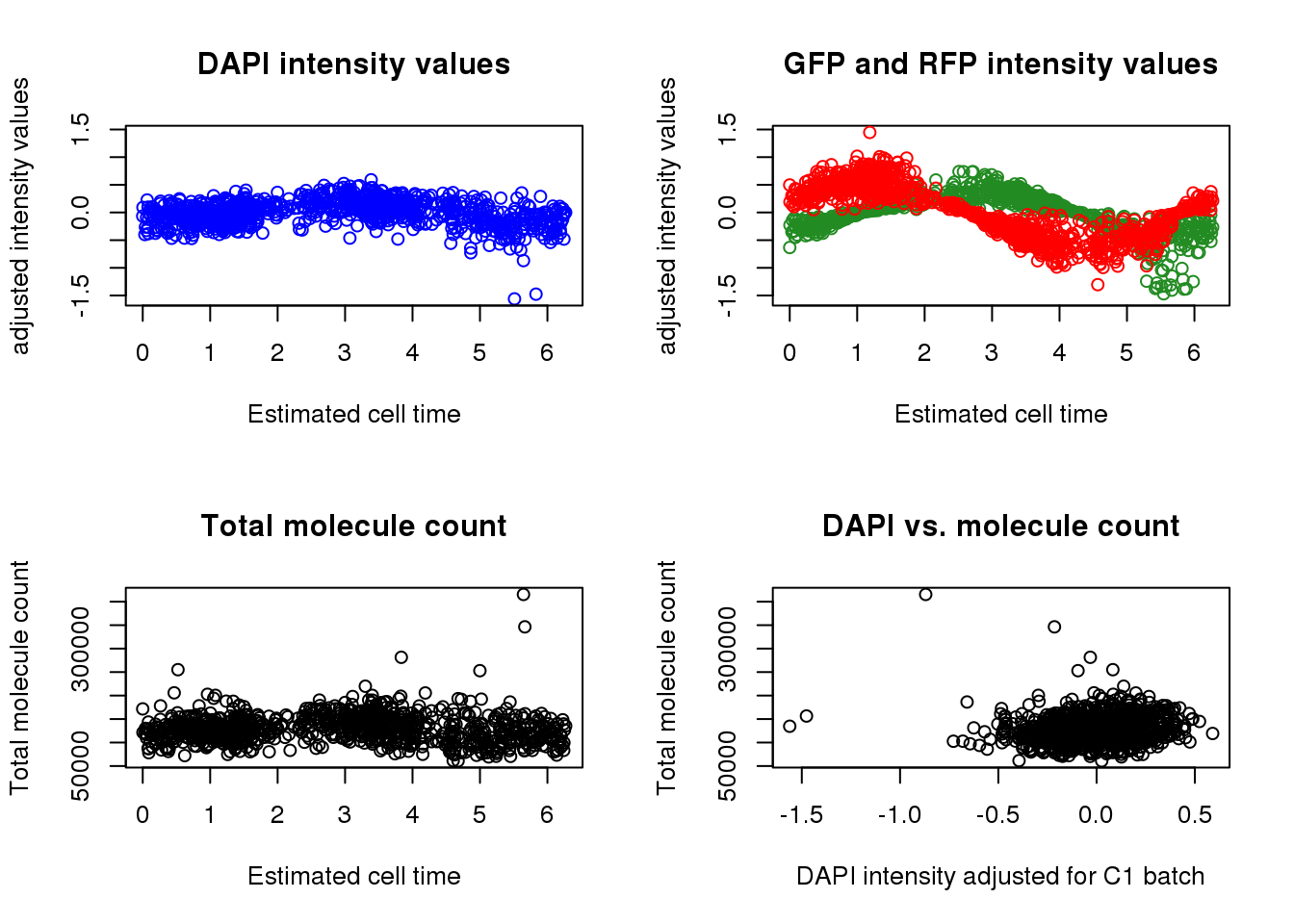
Test the association between total sample molecule count and DAPI.
After excluding outliers, pearson correlation is .2
Consider lm(molecules ~ dapi). The adjusted R-squared is .04
Consider lm(log10(molecules) ~ dapi). The adjusted R-squared is .04
Weak linear trend between molecule count and DAPI…
xy <- data.frame(dapi=pdata.adj$dapi.median.log10sum.adjust,
                 molecules=pdata$molecules)
xy <- subset(xy, molecules < 2*10^5 & dapi > -1)

fit <- lm(log10(molecules)~dapi, data=xy)
summary(fit)
Call:
lm(formula = log10(molecules) ~ dapi, data = xy)

Residuals:
      Min        1Q    Median        3Q       Max
-0.316134 -0.056187  0.007504  0.060388  0.225894

Coefficients:
            Estimate Std. Error  t value Pr(>|t|)
(Intercept) 5.098818   0.002783 1832.186  < 2e-16 ***
dapi        0.082510   0.013209    6.246 6.27e-10 ***
---
Signif. codes:  0 '***' 0.001 '**' 0.01 '*' 0.05 '.' 0.1 ' ' 1

Residual standard error: 0.08695 on 975 degrees of freedom
Multiple R-squared:  0.03848,   Adjusted R-squared:  0.03749
F-statistic: 39.02 on 1 and 975 DF,  p-value: 6.268e-10
fit <- lm(molecules~dapi, data=xy)
summary(fit)
Call:
lm(formula = molecules ~ dapi, data = xy)

Residuals:
   Min     1Q Median     3Q    Max
-67799 -17713   -348  16665  73746

Coefficients:
            Estimate Std. Error t value Pr(>|t|)
(Intercept) 128117.8      793.7 161.415  < 2e-16 ***
dapi         23538.3     3767.5   6.248 6.21e-10 ***
---
Signif. codes:  0 '***' 0.001 '**' 0.01 '*' 0.05 '.' 0.1 ' ' 1

Residual standard error: 24800 on 975 degrees of freedom
Multiple R-squared:  0.03849,   Adjusted R-squared:  0.03751
F-statistic: 39.03 on 1 and 975 DF,  p-value: 6.211e-10
par(mfrow=c(1,2))
plot(x=xy$dapi, y = xy$molecules,
xlab = "DAPI intensity", ylab = "Total molecule count",
main = "DAPI vs. molecule count \n adj-Rsq = .04")
abline(lm(molecules~dapi, data=xy), col = "red")
plot(x=xy$dapi, y = log10(xy$molecules),
xlab = "DAPI intensity", ylab = "log10 total molecule count",
main = "DAPI vs. log10 molecule count \n adj-Rsq = .04")
abline(lm(log10(molecules)~dapi, data=xy), col = "red")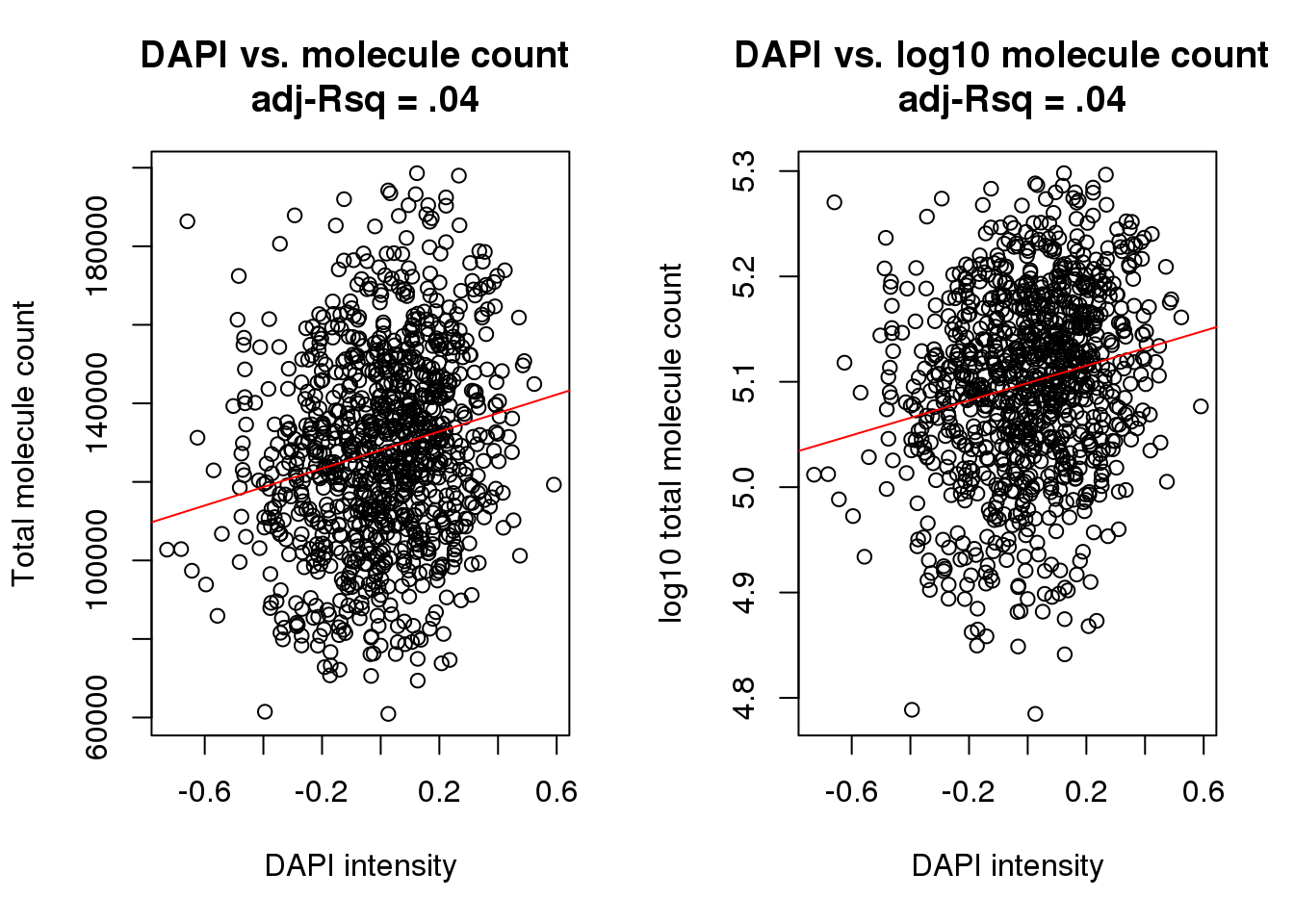
cor(xy$dapi, xy$molecules, method = "pearson")[1] 0.1962001Session information
sessionInfo()R version 3.4.1 (2017-06-30)
Platform: x86_64-redhat-linux-gnu (64-bit)
Running under: Scientific Linux 7.2 (Nitrogen)
Matrix products: default
BLAS/LAPACK: /usr/lib64/R/lib/libRblas.so
locale:
[1] LC_CTYPE=en_US.UTF-8 LC_NUMERIC=C
[3] LC_TIME=en_US.UTF-8 LC_COLLATE=en_US.UTF-8
[5] LC_MONETARY=en_US.UTF-8 LC_MESSAGES=en_US.UTF-8
[7] LC_PAPER=en_US.UTF-8 LC_NAME=C
[9] LC_ADDRESS=C LC_TELEPHONE=C
[11] LC_MEASUREMENT=en_US.UTF-8 LC_IDENTIFICATION=C
attached base packages:
[1] parallel stats graphics grDevices utils datasets methods
[8] base
other attached packages:
[1] circular_0.4-93 Biobase_2.38.0 BiocGenerics_0.24.0
loaded via a namespace (and not attached):
[1] Rcpp_0.12.16 mvtnorm_1.0-7 digest_0.6.15 rprojroot_1.3-2
[5] backports_1.1.2 git2r_0.21.0 magrittr_1.5 evaluate_0.10.1
[9] stringi_1.1.7 boot_1.3-19 rmarkdown_1.9 tools_3.4.1
[13] stringr_1.3.0 yaml_2.1.18 compiler_3.4.1 htmltools_0.3.6
[17] knitr_1.20 This R Markdown site was created with workflowr