Creating Custom Cluster Files in GenomeStudio
Jenny Sjaarda
Last updated: 2019-12-02
Checks: 2 0
Knit directory: PSYMETAB/
This reproducible R Markdown analysis was created with workflowr (version 1.5.0). The Checks tab describes the reproducibility checks that were applied when the results were created. The Past versions tab lists the development history.
Great! Since the R Markdown file has been committed to the Git repository, you know the exact version of the code that produced these results.
Great! You are using Git for version control. Tracking code development and connecting the code version to the results is critical for reproducibility. The version displayed above was the version of the Git repository at the time these results were generated.
Note that you need to be careful to ensure that all relevant files for the analysis have been committed to Git prior to generating the results (you can use wflow_publish or wflow_git_commit). workflowr only checks the R Markdown file, but you know if there are other scripts or data files that it depends on. Below is the status of the Git repository when the results were generated:
Ignored files:
    Ignored:    .drake/
    Ignored:    data/processed/
    Ignored:    data/raw/

Untracked files:
    Untracked:  analysis/QC/
    Untracked:  post_imputation_qc.log
    Untracked:  pre_impute_qc.out
    Untracked:  qc_part2.out

Unstaged changes:
    Deleted:    pre_imputation_qc.out
    Deleted:    qc_part1.out
Note that any generated files, e.g. HTML, png, CSS, etc., are not included in this status report because it is ok for generated content to have uncommitted changes.
These are the previous versions of the R Markdown and HTML files. If you’ve configured a remote Git repository (see ?wflow_git_remote), click on the hyperlinks in the table below to view them.
| File | Version | Author | Date | Message |
|---|---|---|---|---|
| Rmd | 0dd02a7 | Jenny | 2019-12-02 | modify website |
Notes from Illumina webinar: GenomeStudio Genotyping: Creating Custom Cluster Files for Infinium Arrays.
Background and raw genotype data:
- Scanner detects red and green fluorescent intenseities for each locaus (A and B) to produce genotyping data (intensity data files - idats).
- GenomeStudio converts A and B color channel signals into genoype calls.
- A and B intensity plots (A vs. B) are transformed into polar coordinates plots (theta vs. R, where theta is the angle from the line Y=0 [x-axis] to a given point i (A,B) and R = sum of A and B signal intensities).
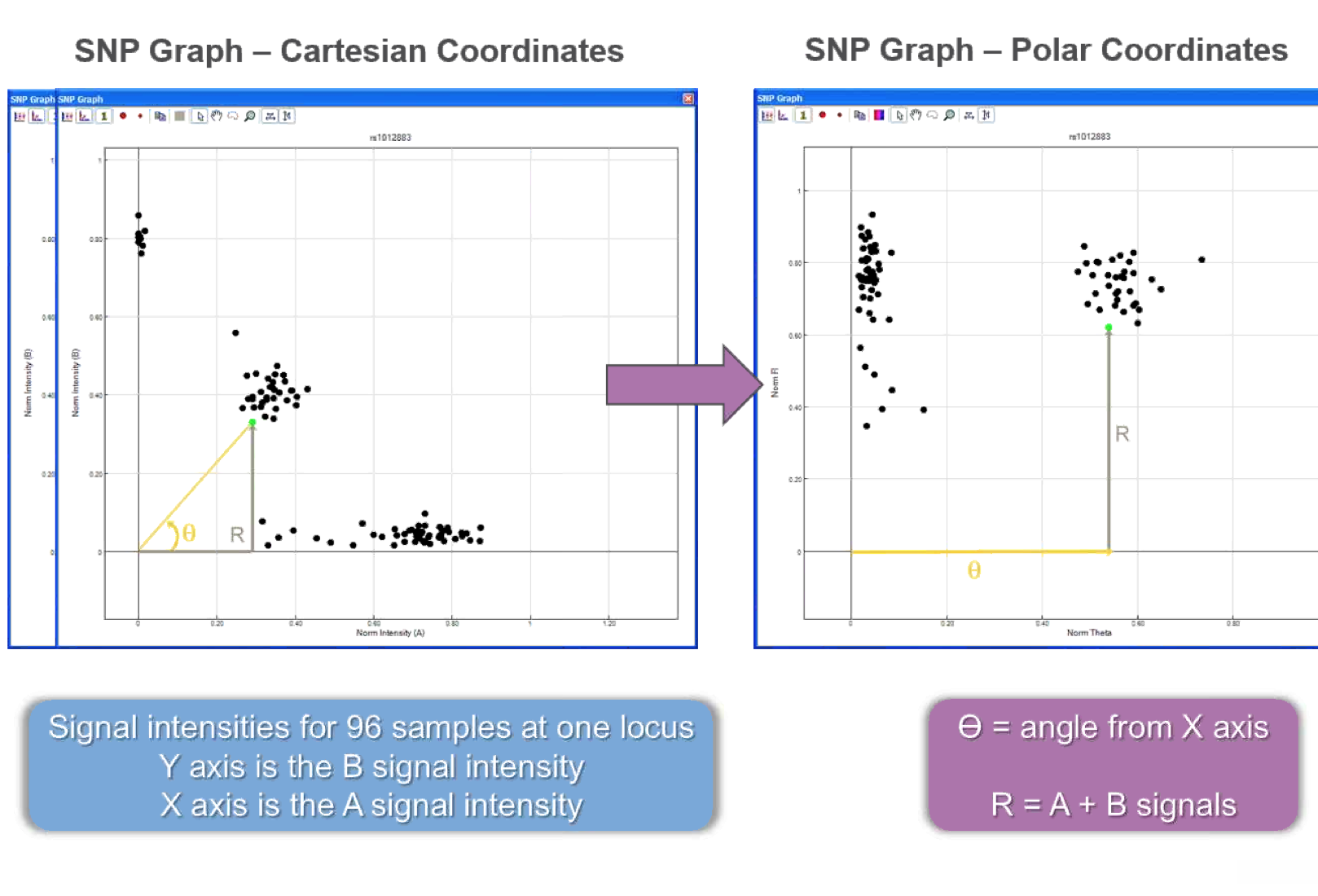
- GS uses algorithms to create clusters and assign genotypes.
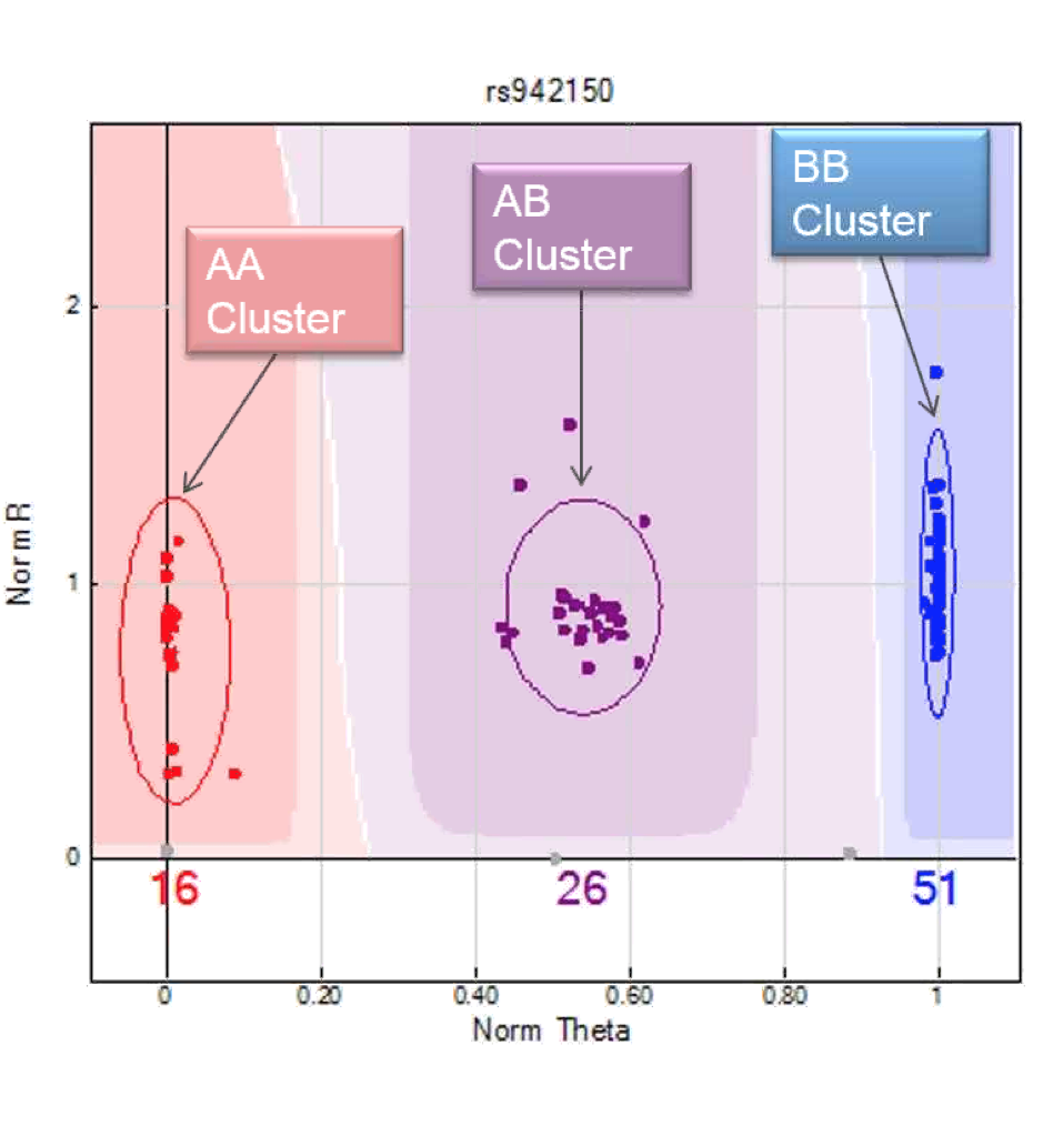
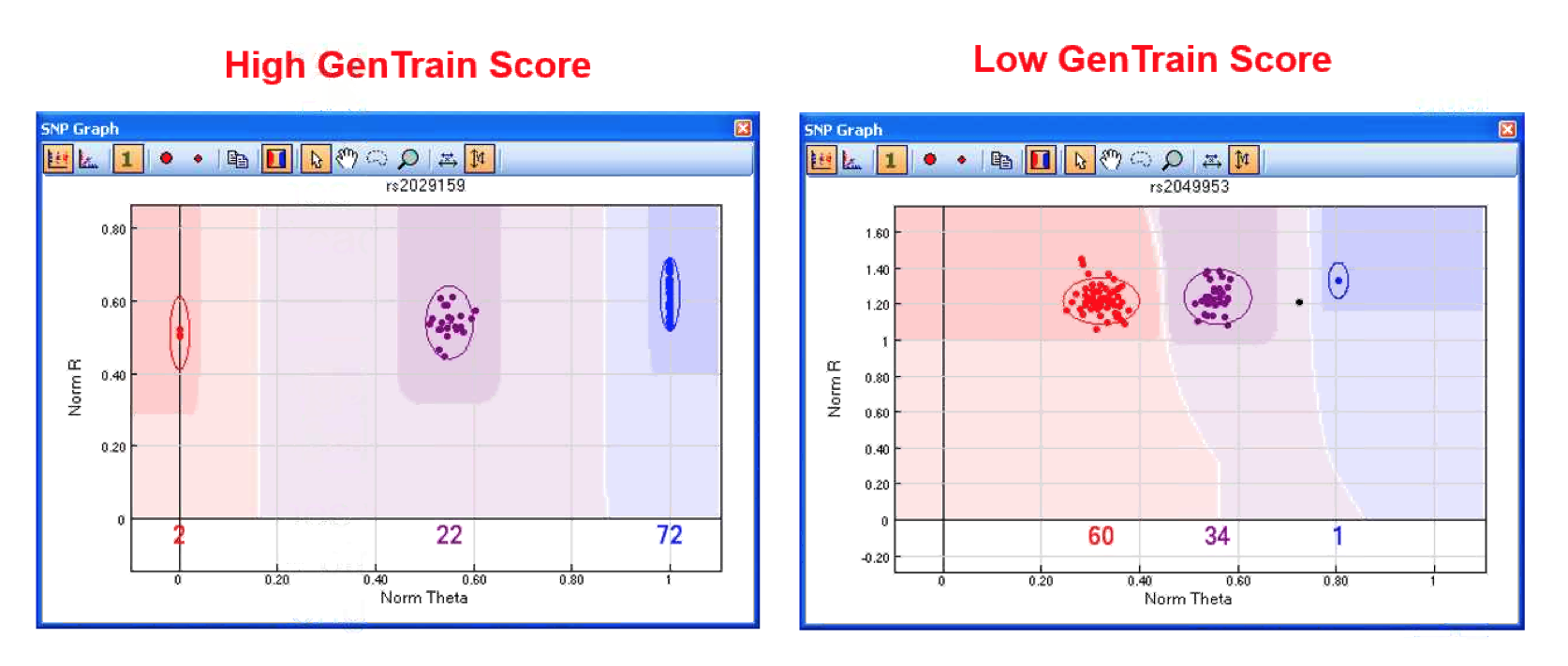
- Clustering algorithm GenTrain surveys data to determine shape of genotype cluster (3 clusters expected), algorithm works in 3 steps (SNP specific):
- Preliminary clustering based on samples, looks for groups.
- Assigns 3 clusters (AA/AB/BB).
- Scores them based on tighteness and spread between them and HW, perfect GenTrain score = 1.
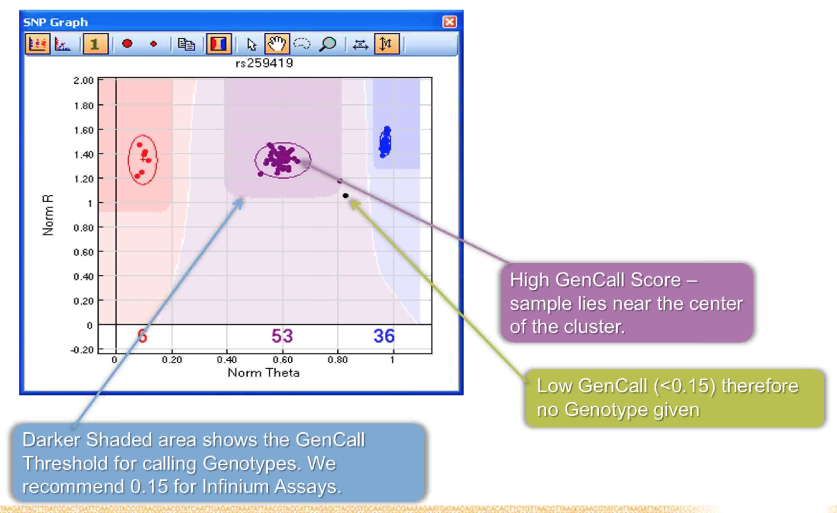
- Calling algorithm GenCall determines which genotype bin each data point belongs to after clustered are defined.
- GenCall score is SNP and sample specific, measures how well a smaple fits into a given cluster.
- SNP with poor GenTrain score then this SNP will also have low GenCall scores.
- Threshold for calling genotypes is recommended at 0.15.
Cluster files:
- Matrices, with one row per SNP with the following columns:
- Cluster positions: mean and SD of R and Theta for each AA, AB, BB cluster in normalized coordinates for every SNP.
- Cluster score information, i.e. GenTrain score.
- Cluster seperation.

- Cluster file (.egt) and manifest file (.bpm) are needed to define genotypes from intensity files (.idats).
- Standard cluster files are provided with each version of an array.
- Reclustering some or all SNPs will make your calls more accurate (since they are based on your data not a reference panel).
Designing a custom cluster file:
- Sample choice:
- Use normal samples (i.e. controls)
- Samples of comparable, good quality
- >100 individauls
- Conditions:
- >3 runs
- >3 reagent lots
- Representative number of operators/technicians/robtots
Creating a cluster file:
- Cluster:
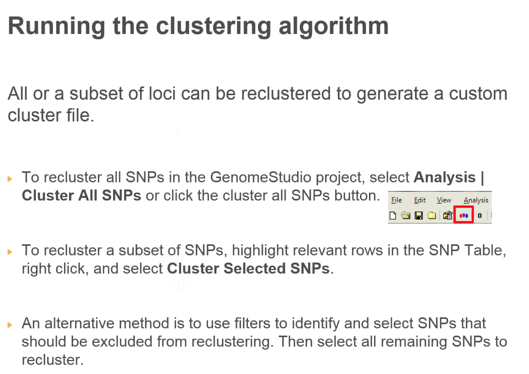
- Cluster all SNPs (takes a long time)
- Evaluate samples and remove outliers
- Recluster:
- Cluster sex chromosomes
- Cluster autosomes
- Review and edit:
- Use filters and score to evaluate SNPs
- Correct or zero SNPs as needed
See technical note with additional details.