Last updated: 2020-07-28

Checks: 6 1

Knit directory: jesslyn_ovca/analysis/

This reproducible R Markdown analysis was created with workflowr (version 1.6.2). The Checks tab describes the reproducibility checks that were applied when the results were created. The Past versions tab lists the development history.

R Markdown file: uncommitted changes

The R Markdown file has unstaged changes. To know which version of the R Markdown file created these results, you’ll want to first commit it to the Git repo. If you’re still working on the analysis, you can ignore this warning. When you’re finished, you can run wflow_publish to commit the R Markdown file and build the HTML.

Environment: empty

Great job! The global environment was empty. Objects defined in the global environment can affect the analysis in your R Markdown file in unknown ways. For reproduciblity it’s best to always run the code in an empty environment.

Seed: set.seed(20200713)

The command set.seed(20200713) was run prior to running the code in the R Markdown file. Setting a seed ensures that any results that rely on randomness, e.g. subsampling or permutations, are reproducible.

Session information: recorded

Great job! Recording the operating system, R version, and package versions is critical for reproducibility.

Cache: none

Nice! There were no cached chunks for this analysis, so you can be confident that you successfully produced the results during this run.

File paths: relative

Great job! Using relative paths to the files within your workflowr project makes it easier to run your code on other machines.

Repository version: 35c7947

Great! You are using Git for version control. Tracking code development and connecting the code version to the results is critical for reproducibility.

The results in this page were generated with repository version 35c7947. See the Past versions tab to see a history of the changes made to the R Markdown and HTML files.

Note that you need to be careful to ensure that all relevant files for the analysis have been committed to Git prior to generating the results (you can use wflow_publish or wflow_git_commit). workflowr only checks the R Markdown file, but you know if there are other scripts or data files that it depends on. Below is the status of the Git repository when the results were generated:


Ignored files:
    Ignored:    .DS_Store
    Ignored:    .Rhistory
    Ignored:    .Rproj.user/
    Ignored:    analysis/.DS_Store
    Ignored:    code/.DS_Store
    Ignored:    data/.DS_Store
    Ignored:    data/HTAPP/
    Ignored:    data/Izar_2020/
    Ignored:    data/gene_lists/.DS_Store
    Ignored:    data/gene_lists/extra/.DS_Store
    Ignored:    jesslyn_plots/
    Ignored:    mike_plots/
    Ignored:    old/.DS_Store
    Ignored:    renv/.DS_Store
    Ignored:    renv/library/
    Ignored:    renv/python/
    Ignored:    renv/staging/
    Ignored:    vignettes/

Unstaged changes:
    Modified:   analysis/02.1_Izar2020_SS2_DEAnalysis.Rmd
    Modified:   analysis/03.1_Izar2020_PDX_DEAnalysis.Rmd
    Modified:   analysis/index.Rmd
    Modified:   old/edited/02_Izar2020_SS2_Load_Plots.Rmd

Note that any generated files, e.g. HTML, png, CSS, etc., are not included in this status report because it is ok for generated content to have uncommitted changes.

These are the previous versions of the repository in which changes were made to the R Markdown (analysis/02.1_Izar2020_SS2_DEAnalysis.Rmd) and HTML (docs/02.1_Izar2020_SS2_DEAnalysis.html) files. If you’ve configured a remote Git repository (see ?wflow_git_remote), click on the hyperlinks in the table below to view the files as they were in that past version.

File	Version	Author	Date	Message
Rmd	35c7947	jgoh2	2020-07-27	SS2 Analysis Part 1 and 2
Rmd	e27cfd1	jgoh2	2020-07-22	Moved files out of the analysis folder + AddModulescore in read_Izar_2020.R
Rmd	527247a	jgoh2	2020-07-20	Reorganize SS2 code and add to the analysis folder

IZAR 2020 SS2 (COHORT 2) DATA DIFFERANTIAL EXPRESISON ANALYSIS

OVERVIEW

The SS2 data from Izar2020 consists of cells from 14 ascites samples from 6 individuals:
- selected for malignant EPCAM+CD24+ cells by fluorophore-activated cell sorting into 96-well plates
- Includes both malignant and nonmalignant populations but differs from 10X data - examines malignant ascites more closely.
- We are only interested in the malignant ascites population, specifically samples from patient 8 and 9 because they are the only patients that have samples from different treatment statuses:
- Treatment naive (p.0)
- On-treatment (p.1 and p.2)
- Did not specify like 10X data whether p.1 is after initial chemotherapy and p.2 is on-treatment (Clinical status at time of sample collection obtained from patients 8 and 9 is “Recurent”)
In our 3-part analysis of the Izar 2020 SS2 data, we are interested in identifying differentially expressed genes and hallmark genesets between treatment statuses within patients 8 and 9
We split our SS2 analysis into three parts:
1. Load Data and Create SS2 Seurat Object
  1. The code to this part of our analysis is in the read_Izar_2020.R file in the code folder. During this part of our analysis we:
    1. Load in SS2 count matrix and Create Seurat Object
    2. Assign Metadata identities including:
      - Patient ID
      - Time
      - Sample ID
      - Treatment Status
    3. Score cells for cell cycle and hallmark genesets - Note: It does not matter whether we call AddModuleScore before or after subsetting and scaling each model because AddModuleScore uses the data slot.
    4. Save Seurat Object
2. Process Data and Exploratory Data Analysis
  1. The code to this part of our analysis can be found in the 03_Izar2020_SS2_Load_Plots.Rmd file in the old/edited folder. During this part of our analysis we:
    1. Load in SS2 Seurat Object from Part 1 and subset for Malignant cells then for patient 8 and 9. Continue analysis separately for each patient.
    2. Scale and FindVariableFeatures (prepares data for dimensionality reduction)
    3. Dimensionality Reduction (PCA + UMAP)
    4. Visualize how cells separate based on metadata identities via UMAP
      - Intermodel heterogeneity: How do cells separate by model?
      - Intramodel heterogeneity:
        
        How do cells separate by treament status?
        
        How do cells separate by cell cycle phase?
    5. Compute summary metrics for SS2 data such as:
      - Number of cells per patient per treatment
      - Number of cells per treatment per cell cycle phase
    6. Save Seurat Objects
3. DE Analysis
  1. TYPE #1 DE ANALYSIS: Visualizing and Quantifying Differentially Expression on Predefined GO Genesets
    1. Violin Plots and UMAP
    2. Gene Set Enrichment Analysis (GSEA)
  2. TYPE #2 DE ANALYSIS: Finding DE Genes from scratch
    1. Volcano Plots
  3. CELL CYCLE ANALYSIS
    1. Evaluate the idea that cell cycle might influence expression of signatures

This is the third part of our 3-part analysis of the Izar 2020 SS2 (Cohort 2) data.

STEP 1 LOAD SEURAT OBJECT

# Load packages
source(here::here('packages.R'))

#Read in SS2 RDS object
SS2Malignant = readRDS(file = "data/Izar_2020/jesslyn_SS2Malignant_processed.RDS")
SS2Malignant.8 = readRDS(file = "data/Izar_2020/jesslyn_SS2Malignant8_processed.RDS")
SS2Malignant.9 = readRDS(file = "data/Izar_2020/jesslyn_SS2Malignant9_processed.RDS")

#Read in hallmarks of interest
hallmark_names = read_lines("data/gene_lists/hallmarks.txt")
hallmark.list <- vector(mode = "list", length = length(hallmark_names) + 2)
names(hallmark.list) <- c(hallmark_names, "GO.OXPHOS", "KEGG.OXPHOS")
for(hm in hallmark_names){
  file <- read_lines(glue("data/gene_lists/hallmarks/{hm}_updated.txt"), skip = 1)
  hallmark.list[[hm]] <- file
}

hallmark.list[["GO.OXPHOS"]] <- read_lines("data/gene_lists/extra/GO.OXPHOS.txt", skip = 1)
hallmark.list[["KEGG.OXPHOS"]] <- read_lines("data/gene_lists/extra/KEGG.OXPHOS.txt", skip = 2)

#center module and cell cycle scores and reassign to the metadata of each Seurat object
hm.names <- names(SS2Malignant@meta.data)[14:51]

for(i in hm.names){
    SS2Malignant.hm.centered <- scale(SS2Malignant[[i]], center = TRUE, scale = FALSE)
    SS2Malignant <- AddMetaData(SS2Malignant, SS2Malignant.hm.centered, col.name = glue("{i}.centered"))
    
    SS2Malignant8.hm.centered <- scale(SS2Malignant.8[[i]], center = TRUE, scale = FALSE)
    SS2Malignant.8 <- AddMetaData(SS2Malignant.8, SS2Malignant8.hm.centered, col.name = glue("{i}.centered"))
    
    SS2Malignant9.hm.centered <- scale(SS2Malignant.9[[i]], center = TRUE, scale = FALSE)
    SS2Malignant.9 <- AddMetaData(SS2Malignant.9, SS2Malignant9.hm.centered, col.name = glue("{i}.centered"))
}

STEP 2 DE ANALYSIS #1. VISUALIZING AND QUANTIFYING DE HALLMARK GENESETS

QUESTION Are modules (OXPHOS and UPR) differentially expressed across treatment conditions within each patient?
HYPOTHESIS We hypothesize that the on-treatment time-points (p.1 and p.2) will express enriched levels of OXPHOS and UPR hallmarks relative to cells treatment-naive time-point (p.0). We are not so sure what to expect between p.1 and p.2 on-treatment samples because we are not told how the two samples are different in terms of their treatment status.
- APPROACH #1 Violin Plots and UMAP
  - Visualize differences in hallmark score across treatment conditions with:
    - UMAP by treatment vs. UMAP by hallmark score
    - Violin Plot (center module scores at 0)
  - Statistical test (wilcoxon rank sum test): is the difference in hallmark score across treatment conditions statistically significant?

hms.centered <- c("KEGG.OXPHOS36.centered", "HALLMARK_UNFOLDED_PROTEIN_RESPONSE33.centered")

#UMAP 
SS2.names <- c("SS2 Malignant Patient 8", "SS2 Malignant Patient 9")
SS2s <- c(SS2Malignant.8, SS2Malignant.9)
UMAP.plots <- vector("list", length(SS2s))
names(UMAP.plots) <- SS2.names

for (i in 1:length(SS2s)){
  obj <- SS2s[[i]]
  name <- SS2.names[[i]]
  numCells = nrow(obj@meta.data)
  
  umap <- UMAPPlot(obj, group.by = "sample") + 
    labs(title = glue("{name} UMAP by Sample"), subtitle = glue("Number of cells in {name}: {numCells}")) +
    theme(plot.title = element_text(size = 10), plot.subtitle = element_text(size = 8))
  
  p <- FeaturePlot(obj, features = hms.centered, combine = FALSE)
  p[[1]] <- p[[1]] + labs(title = glue("{name} UMAP by KEGG Oxphos Scores")) +
    theme(plot.title = element_text(size = 10))
  p[[2]] <- p[[2]] + labs(title = glue("{name} UMAP by HALLMARK UPR Scores")) + 
    theme(plot.title = element_text(size = 10))
  
  UMAP.plots[[name]] <- umap + p[[1]] + p[[2]]
}

UMAP.plots[["SS2 Malignant Patient 8"]]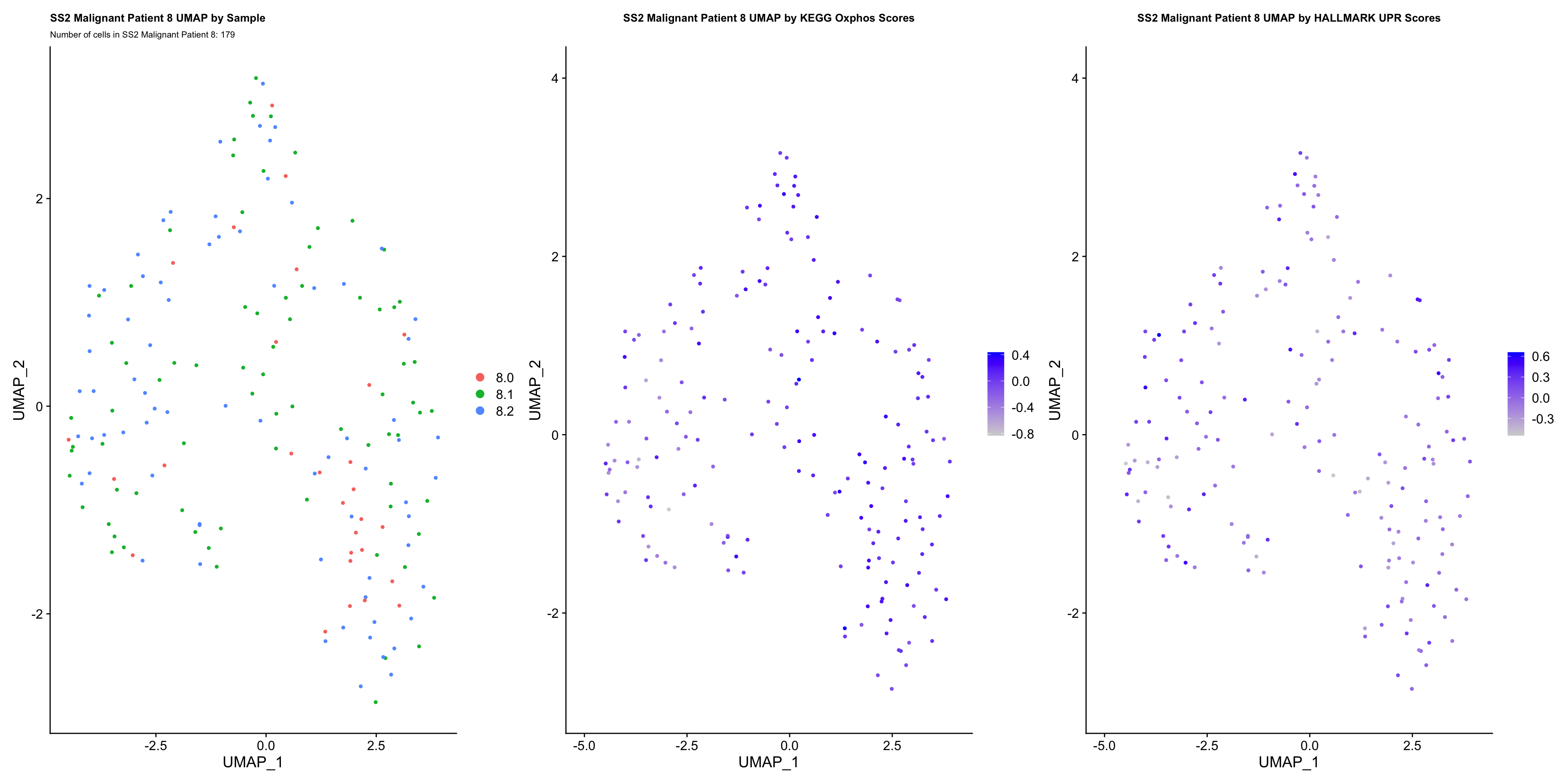

UMAP.plots[["SS2 Malignant Patient 9"]]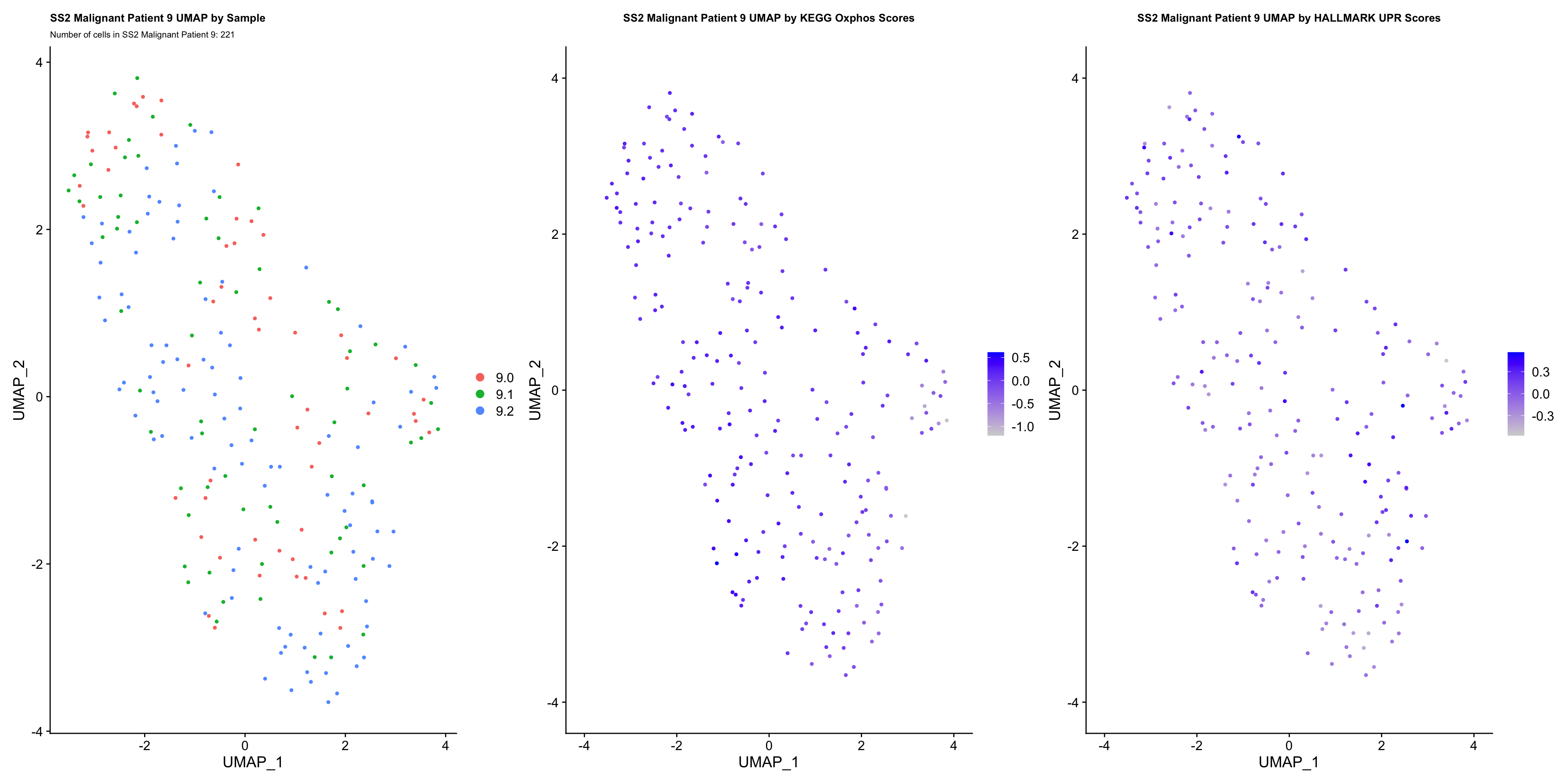

OBSERVATIONS
- Since cells do not separate by treatment status, it is difficult to determine whether there is a correlation between treatment condition and hallmark scores based on our UMAP visualization.
- We therefore try to visualize DE hallmark scores across treatment conditions with VlnPlots

#VlnPlot
SS2.names <- c("SS2 Malignant Patient 8", "SS2 Malignant Patient 9")
SS2s <- c(SS2Malignant.8, SS2Malignant.9)
Vln.plots <- vector("list", length(SS2s))
names(UMAP.plots) <- SS2.names
patient <- c("8", "9")

for (i in 1:length(SS2s)){
  obj <- SS2s[[i]]
  name <- SS2.names[[i]]
  numCells <- nrow(obj@meta.data)
  
  p <- VlnPlot(obj, features = hms.centered, group.by = "sample", pt.size = 0, combine = F)
  p[[1]] <- p[[1]] + labs(title = glue("{name} OXPHOS scores across treatment"), x = name, subtitle = glue("Number of cells in {name}: {numCells}"), caption = "www.gsea-msigdb.org: KEGG_OXIDATIVE_PHOSPHORYLATION") +
    theme(plot.title = element_text(size = 10), plot.caption = element_text(size = 10)) + 
    geom_boxplot(width = 0.15, position = position_dodge(0.9), alpha = 0.3, show.legend = F) + 
    geom_text(label = paste(sum(str_detect(obj$sample, "[:digit:].0")), "cells"), x = glue("{patient[[i]]}.0"), y = min(obj$KEGG.OXPHOS36.centered) -0.03) + 
    geom_text(label = paste(sum(str_detect(obj$sample, "[:digit:].1")), "cells"), x = glue("{patient[[i]]}.1"), y = min(obj$KEGG.OXPHOS36.centered) - 0.03) + 
    geom_text(label = paste(sum(str_detect(obj$sample, "[:digit:].2")), "cells"), x = glue("{patient[[i]]}.2"), y = min(obj$KEGG.OXPHOS36.centered) - 0.03)
  
  p[[2]] <- p[[2]] + labs(title = glue("{name} UPR scores across treatment"), x = name, caption = "www.gsea-msigdb.org: HALLMARK_UNFOLDED_PROTEIN_RESPONSE") +
    theme(plot.title = element_text(size = 10), plot.caption = element_text(size = 10)) + 
    geom_boxplot(width = 0.15, position = position_dodge(0.9), alpha = 0.3, show.legend = F)
  p <- p[[1]] + p[[2]] + plot_layout(guides= 'collect')
  
  Vln.plots[[name]] <- p
}

Vln.plots[["SS2 Malignant Patient 8"]]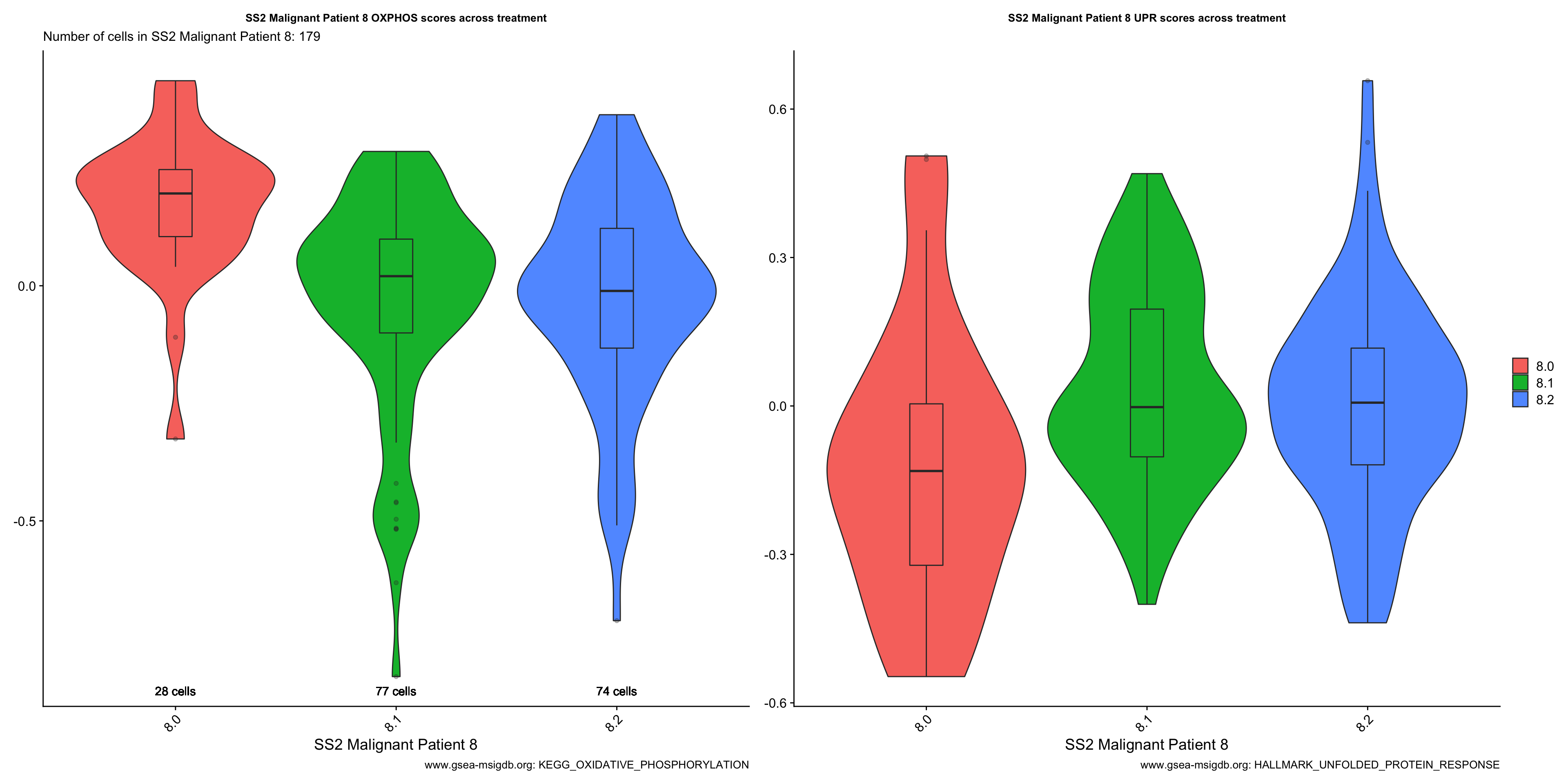

Vln.plots[["SS2 Malignant Patient 9"]]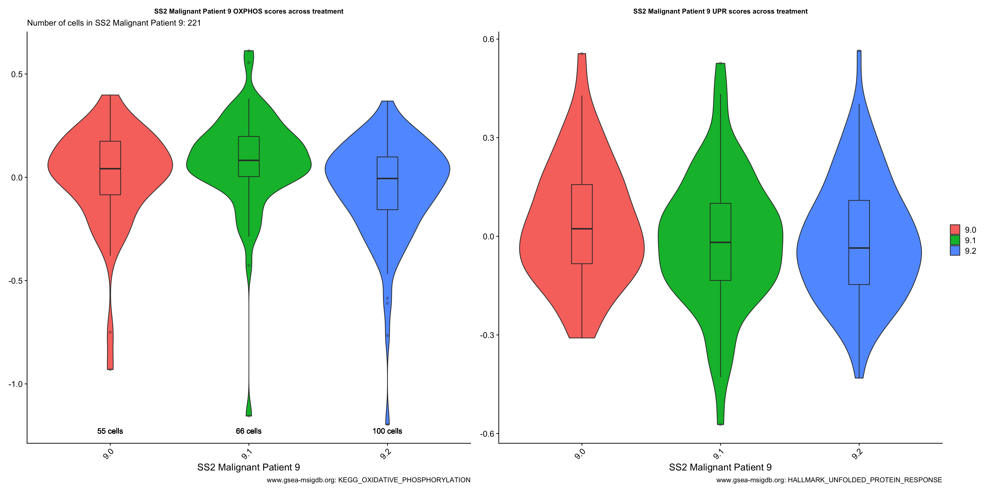

OBSERVATIONS
- Patient 8
  - OXPHOS: Sample 8.0 > 8.1 > 8.2 (does not support our hypothesis)
  - UPR: Sample 8.2 > 8.1 > 8.0
- Patient 9
  - OXPHOS: Sample 9.1 > 9.0 > 9.2 (supports our hypothesis)
  - UPR: Sample 9.0 > 9.1 > 9.2 (does not support our hypothesis)
Overall trend of OXPHOS and UPR scores across treatment time-point within each patient does not support our hypothesis that On-treatment samples (esp. 8.1 and 9.1) will express higher levels of these genes relative to Treatment-naive samples.
We now examine the statistical significance of our results.

#Patient 8 ---------------------------------
SS2Malignant8.0 <- subset(SS2Malignant.8, subset = (sample == "8.0"))
SS2Malignant8.1 <- subset(SS2Malignant.8, subset = (sample == "8.1"))
SS2Malignant8.2 <- subset(SS2Malignant.8, subset = (sample == "8.2"))

SS2M8.oxphos.df <- data.frame(
  "p.0vsp.1" = wilcox.test(SS2Malignant8.0$KEGG.OXPHOS36.centered, SS2Malignant8.1$KEGG.OXPHOS36.centered)$p.value, 
  "p.1vsp.2" = wilcox.test(SS2Malignant8.1$KEGG.OXPHOS36.centered, SS2Malignant8.2$KEGG.OXPHOS36.centered)$p.value, 
  "p.0vsp.2" = wilcox.test(SS2Malignant8.0$KEGG.OXPHOS36.centered, SS2Malignant8.2$KEGG.OXPHOS36.centered)$p.value
)

SS2M8.UPR.df <- 
  data.frame(
  "p.0vsp.1" = wilcox.test(SS2Malignant8.0$HALLMARK_UNFOLDED_PROTEIN_RESPONSE33.centered, SS2Malignant8.1$HALLMARK_UNFOLDED_PROTEIN_RESPONSE33.centered)$p.value, 
  "p.1vsp.2" = wilcox.test(SS2Malignant8.1$HALLMARK_UNFOLDED_PROTEIN_RESPONSE33.centered, SS2Malignant8.2$HALLMARK_UNFOLDED_PROTEIN_RESPONSE33.centered)$p.value, 
  "p.0vsp.2" = wilcox.test(SS2Malignant8.0$HALLMARK_UNFOLDED_PROTEIN_RESPONSE33.centered, SS2Malignant8.2$HALLMARK_UNFOLDED_PROTEIN_RESPONSE33.centered)$p.value
)

#Patient 9 ---------------------------------
SS2Malignant9.0 <- subset(SS2Malignant.9, subset = (sample == "9.0"))
SS2Malignant9.1 <- subset(SS2Malignant.9, subset = (sample == "9.1"))
SS2Malignant9.2 <- subset(SS2Malignant.9, subset = (sample == "9.2"))

SS2M9.oxphos.df <- data.frame(
  "p.0vsp.1" = wilcox.test(SS2Malignant9.0$KEGG.OXPHOS36.centered, SS2Malignant9.1$KEGG.OXPHOS36.centered)$p.value, 
  "p.1vsp.2" = wilcox.test(SS2Malignant9.1$KEGG.OXPHOS36.centered, SS2Malignant9.2$KEGG.OXPHOS36.centered)$p.value, 
  "p.0vsp.2" = wilcox.test(SS2Malignant9.0$KEGG.OXPHOS36.centered, SS2Malignant9.2$KEGG.OXPHOS36.centered)$p.value
)

SS2M9.UPR.df <- 
  data.frame(
  "p.0vsp.1" = wilcox.test(SS2Malignant9.0$HALLMARK_UNFOLDED_PROTEIN_RESPONSE33.centered, SS2Malignant9.1$HALLMARK_UNFOLDED_PROTEIN_RESPONSE33.centered)$p.value, 
  "p.1vsp.2" = wilcox.test(SS2Malignant9.1$HALLMARK_UNFOLDED_PROTEIN_RESPONSE33.centered, SS2Malignant9.2$HALLMARK_UNFOLDED_PROTEIN_RESPONSE33.centered)$p.value, 
  "p.0vsp.2" = wilcox.test(SS2Malignant9.0$HALLMARK_UNFOLDED_PROTEIN_RESPONSE33.centered, SS2Malignant9.2$HALLMARK_UNFOLDED_PROTEIN_RESPONSE33.centered)$p.value
)

#combine ------------------------------
SS2.oxphos.DF <- rbind(SS2M8.oxphos.df, SS2M9.oxphos.df)
rownames(SS2.oxphos.DF) <- c("OXPHOS.PATIENT8", "OXPHOS.PATIENT9")

SS2.UPR.DF <- rbind(SS2M8.UPR.df, SS2M9.UPR.df)
rownames(SS2.UPR.DF) <- c("UPR.PATIENT8", "UPR.PATIENT9")

SS2.all.DF <- rbind(SS2.oxphos.DF, SS2.UPR.DF)
DT::datatable(SS2.all.DF) %>% 
  DT::formatRound(names(SS2.all.DF), digits = 7) %>% 
  DT::formatStyle(names(SS2.all.DF), color = DT::styleInterval(0.05, c('red', 'black')))

CONCLUSIONS
- The statistically significant results are (p < 0.05):
  - Patient 8
    - OXPHOS: Sample 8.0 > 8.1 ; 8.0 > 8.2 (does not support our hypothesis)
    - UPR: Sample 8.2 > 8.0 ; 8.1 > 8.0 (supports our hypothesis)
  - Patient 9
    - OXPHOS: Sample 9.1 > 9.2 (supports our hypothesis, but would be better if 9.1 > 9.0 is also statistically significant)
- Interestingly, 2/3 of the statistically significant comparisons support our hypothesis that on-treatment samples should express higher levels of OXPHOS and/or URP relative to the treatment-naive samples.
- We are, however, not sure how to compare between p.1 vs. p.2 because they are both categorized as “on-treatment” and the clinical status of samples obtained from patients 8 and 9 is “Recurrent”, instead of denoting two types of treatment status “Diagnosis/Initial treatment” that corresponds to the two treatment timepoints for the 10X data.

We try to confirm our results again with our second appraoch: GSEA

APPROACH #2 Geneset Enrichment Analysis (GSEA) - GSEA enrichment plots for hallmarks of interest between condition.1 vs. condition.2 - Rank genes and compute GSEA enrichment scores - Statistical test: how significant are the enrichment scores?

have not finalized the statistical test and ranking method to use for GSEA

STEP 3 DE ANALYSIS #2. IDENTIFYING INDIVIDUAL DE GENES

have not finalized the statistical test to use for volcano plot (need to match what we use for GSEA)

STEP 4 CELL CYCLE ANALYSIS

QUESTION #1 Are more cells at different cell cycle phases between treatments?
HYPOTHESIS There should be less cycling cells in the on-treatment conditions (p.1 and p.2) relative to the treatment-naive condition (p.0)
- APPROACH Violin Plots and UMAP
  - Visualize differences in cell cycle score across treatment conditions with:
    - Stacked Bar Plot
    - UMAP by treatment vs. UMAP by cell cycle phase vs. UMAP by S and G2M Score
    - Violin Plot
  - Statistical test: is the difference in cell cycle scores across treatment conditions statistically significant.

#Stacked Bar Plot --------------------------
bar.plots <- vector("list", length = 3)
names(bar.plots) <- SS2.names

for(i in 1:length(SS2s)){
  obj = SS2s[[i]]
  name = SS2.names[[i]]
  numCells = nrow(obj@meta.data)
  
  obj$Phase <- factor(obj$Phase, levels = c("G1", "S", "G2M"))
  t = table(obj$Phase, obj$sample) %>% 
    as.data.frame() %>% 
    rename(Phase = Var1, Sample = Var2, numCells = Freq)

sum = c()
z = 1
while(z < nrow(t)){
    n = t$numCells[z] + t$numCells[z+1] + t$numCells[z+2]
    sum = c(sum, rep(n,3))
    z = z + 3
  }
  
t <- t %>% mutate(total = sum) %>% mutate(percent = (numCells/total)*100)
  
  p = t %>% 
    ggplot(aes(x=Sample, y=percent, fill=Phase)) + 
    geom_bar(stat="identity") + 
    labs(title = glue("{name} % of Cells in Each Cell Cycle Phase/ Treatment"), subtitle = glue("Total # Cells in {name}: {numCells}"), caption = "Labeled by # cells in each phase per treatment") +
    theme(plot.title = element_text(size = 10), plot.subtitle = element_text(size = 10), plot.caption = element_text(size = 8)) +
    geom_text(aes(label = paste(numCells, "cells")), position = "stack", hjust = 0.5, vjust = 2, size = 3, color = "white")
  bar.plots[[i]] <- p
}

bar.plots[["SS2 Malignant Patient 8"]] + bar.plots[["SS2 Malignant Patient 9"]] + plot_layout(guides= 'collect')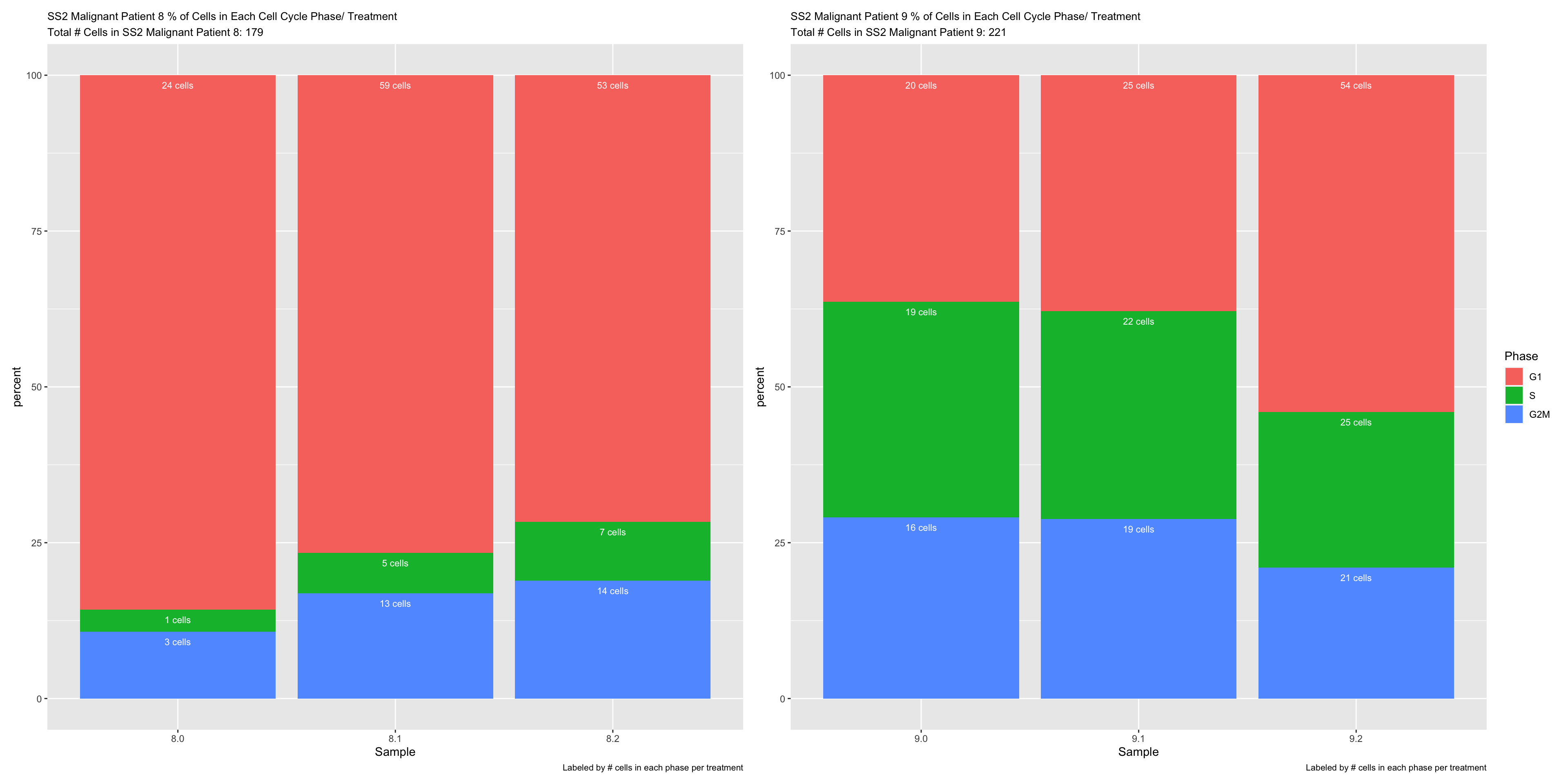

OBSERVATIONS
- Patient 8 % Noncyclying cells 8.0 > 8.1 > 8.2 (does not support our hypothesis, on-treatment samples should have more noncycling cells)
- Patient 9 % Noncycling cells 9.2 > 9.1 > 9.0 (supports our hypothesis, not sure how to interpret 9.2 > 9.1)
- Important to note that we have very little cells in each condition, so we have really little power and the results from our sample may not be representative of the true population.

To investigate this further, we compare PCA by sample vs. PCA by cell cycle phase and scores

#PCA -------------------- (PCA is known to separate cell by cell cycle really well)
ccPCA.plots <- vector("list", length = 3)
names(ccPCA.plots) <- SS2.names

for(i in 1:length(SS2s)){
  obj = SS2s[[i]]
  name = SS2.names[[i]]
  numCells = nrow(obj@meta.data)
  obj$Phase <- factor(obj$Phase, levels = c("G1", "S", "G2M"))
  
  bys <- PCAPlot(obj, group.by = "sample") + 
    labs(title = glue("{name} PCA by sample"), subtitle = glue("Number of cells in {name}: {numCells}")) +
    theme(plot.title = element_text(hjust = 0.5))
  
  bycc <- PCAPlot(obj, group.by = "Phase") + 
    labs(title = glue("{name} PCA by Cell Cycle Phase")) + 
    theme(plot.title = element_text(hjust = 0.5))
  
  byscore <- FeaturePlot(obj, features = c("S.Score", "G2M.Score"), reduction = "pca",combine = FALSE)
  byscore[[1]] <- byscore[[1]] + labs(title = glue("{name} PCA by centered S Score"))
  byscore[[2]] <- byscore[[2]] + labs(title = glue("{name} PCA by centered G2M Score"))
  
  ccPCA.plots[[i]] <- bys + bycc + byscore[[1]] + byscore[[2]]
}

ccPCA.plots[["SS2 Malignant Patient 8"]]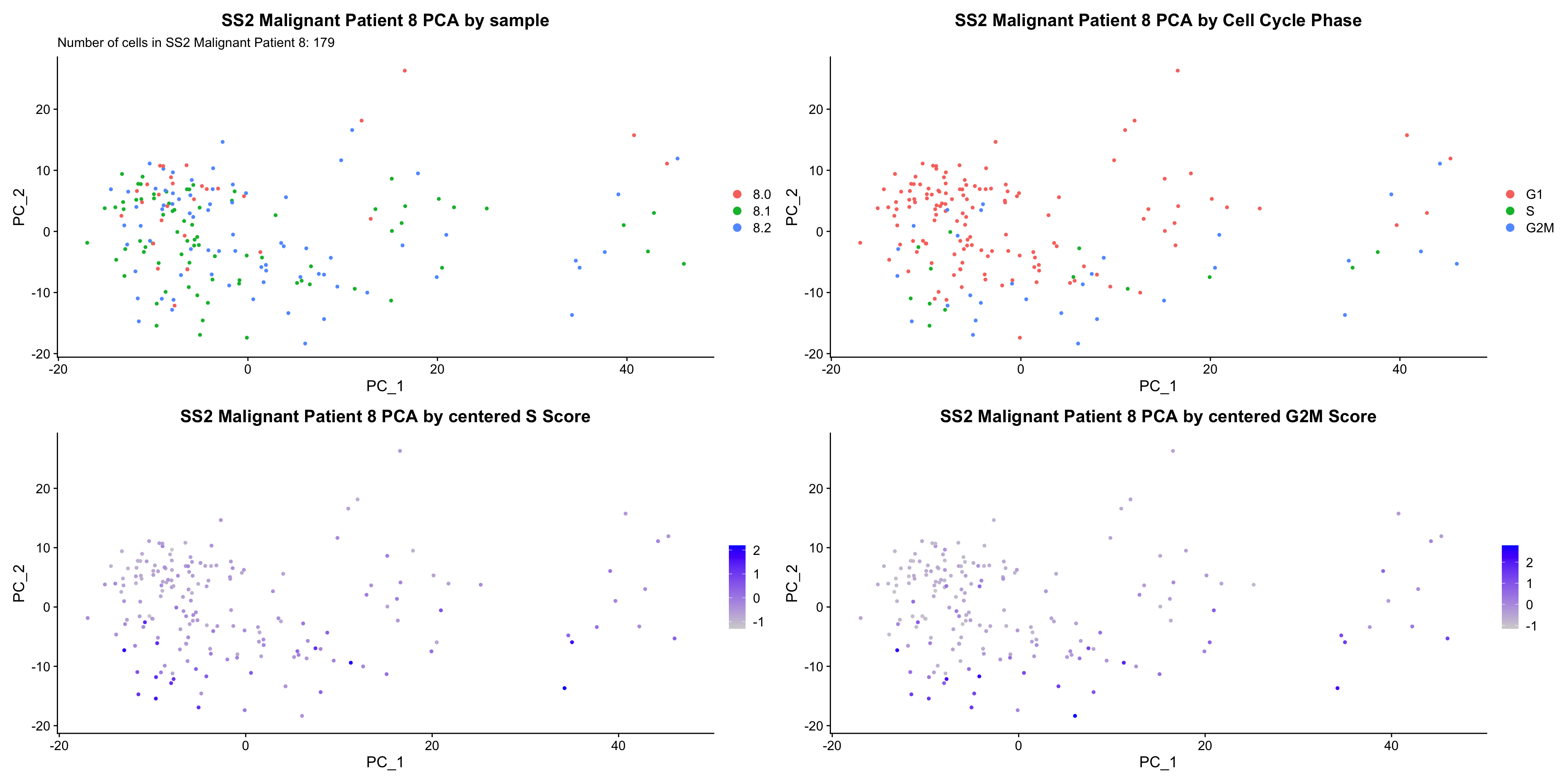

ccPCA.plots[["SS2 Malignant Patient 9"]]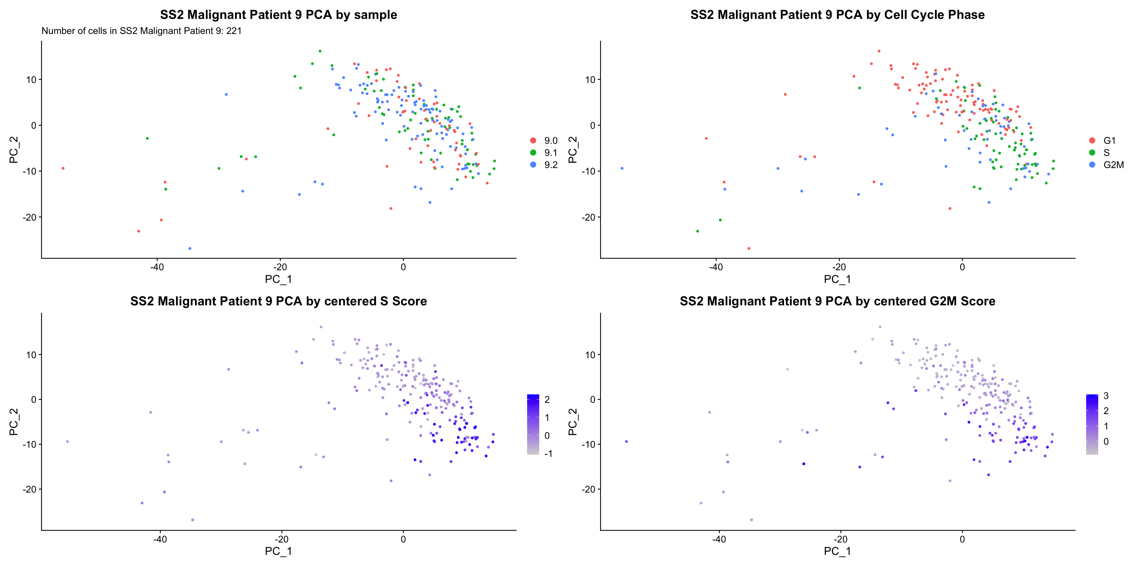

OBSERVATIONS
- No obvious separation by treatment. However, cells in the same cell cycle phase, or those with higher S or G2M score, seem to cluster closer together in PCA space.
- However, it is hard to tell whether there is a correlation between treatment condition and cell cycle phase / score based on these plots. We further investigate this by building violin plots of cell cycle scores separated by treatment status.

#VlnPlot -------------------------
cc.Vln.plots <- vector("list", length = 3)
names(Vln.plots) <- SS2.names

for (i in 1:length(SS2s)){
  obj <- SS2s[[i]]
  name <- SS2.names[[i]]
  numCells = nrow(obj@meta.data)
  p <- VlnPlot(obj, features = c("S.Score.centered", "G2M.Score.centered"), group.by = "sample", pt.size = 0, combine = F)
  p[[1]] <- p[[1]] + labs(title = glue("{name} S.Score across treatment"), x = name, subtitle = glue("Number of cells in {name}: {numCells}")) + 
    geom_boxplot(width = 0.15, position = position_dodge(0.9), alpha = 0.3, show.legend = F) + 
    geom_text(label = paste(sum(str_detect(obj$sample, "[:digit:].0")), "cells"), x = glue("{patient[[i]]}.0"), y = min(obj$S.Score.centered) -0.03) + 
    geom_text(label = paste(sum(str_detect(obj$sample, "[:digit:].1")), "cells"), x = glue("{patient[[i]]}.1"), y = min(obj$S.Score.centered) - 0.03) + 
    geom_text(label = paste(sum(str_detect(obj$sample, "[:digit:].2")), "cells"), x = glue("{patient[[i]]}.2"), y = min(obj$S.Score.centered) - 0.03)
  
  p[[2]] <- p[[2]] + labs(title = glue("{name} G2M.Score across treatment"), x = name) +
    geom_boxplot(width = 0.15, position = position_dodge(0.9), alpha = 0.3, show.legend = F)

  cc.Vln.plots[[name]] <- p[[1]] + p[[2]] + plot_layout(guides= 'collect')
}

cc.Vln.plots[["SS2 Malignant Patient 8"]]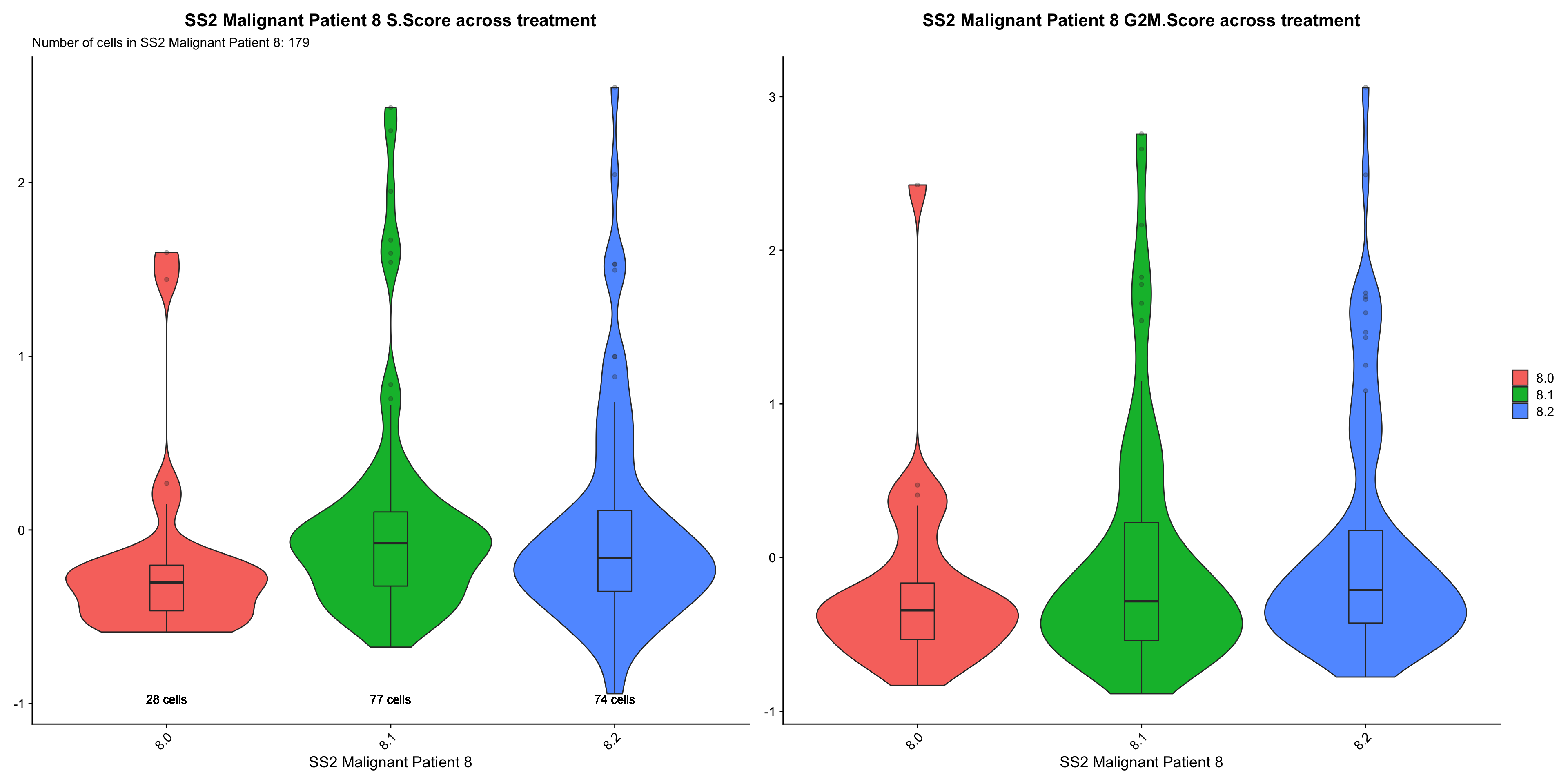

cc.Vln.plots[["SS2 Malignant Patient 9"]]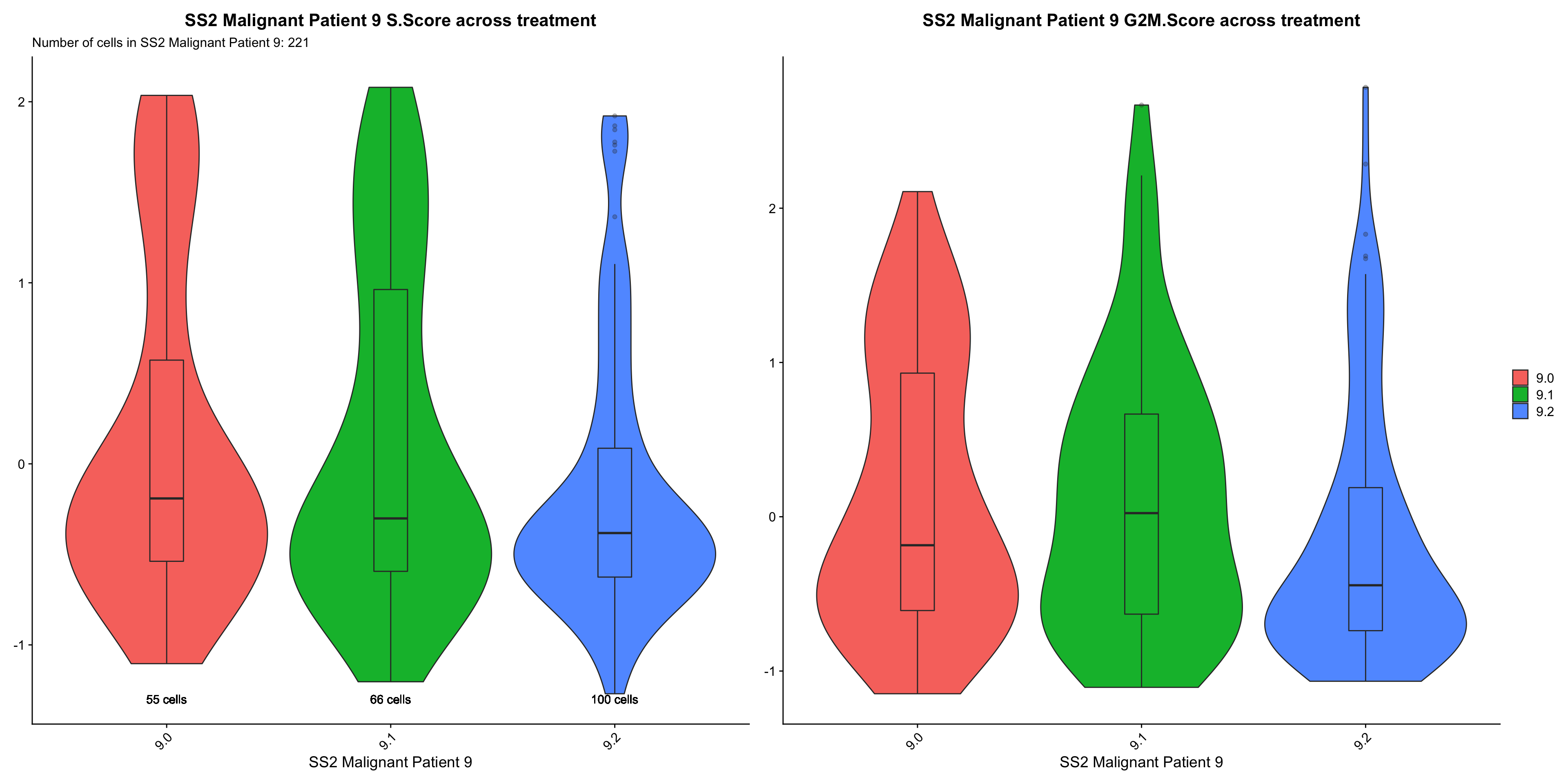

OBSERVATIONS
- Patient 8
  - S.SCORE: Sample 8.1 > 8.2 > 8.0 (does not support our hypothesis, on-treatment samples should have lower S and G2M cycling scores)
  - G2M.SCORE: Sample 8.2 > 8.1 > 8.0 (does not support our hypothesis)
- Patient 9
  - S.SCORE: Sample 9.0 > 9.1 > 9.2 (supports our hypothesis)
  - G2M.SCORE: Sample 9.1 > 9.0 > 9.2 (does not support our hypothesis, 9.1 should have a lower G2M score than 9.0)
Overall trend of S and G2M scores across treatment time-point within each patient does not support our hypothesis that On-treatment samples (esp. 8.1 and 9.1) will express lower levels of these genes relative to Treatment-naive samples.
We now examine which comparison are statistical significance.

#Patient 8 ---------------------------------
SS2M8.S.df <- data.frame(
  "p.0vsp.1" = wilcox.test(SS2Malignant8.0$S.Score.centered, SS2Malignant8.1$S.Score.centered)$p.value, 
  "p.1vsp.2" = wilcox.test(SS2Malignant8.1$S.Score.centered, SS2Malignant8.2$S.Score.centered)$p.value, 
  "p.0vsp.2" = wilcox.test(SS2Malignant8.0$S.Score.centered, SS2Malignant8.2$S.Score.centered)$p.value
)

SS2M8.G2M.df <- 
  data.frame(
  "p.0vsp.1" = wilcox.test(SS2Malignant8.0$G2M.Score.centered, SS2Malignant8.1$G2M.Score.centered)$p.value, 
  "p.1vsp.2" = wilcox.test(SS2Malignant8.1$G2M.Score.centered, SS2Malignant8.2$G2M.Score.centered)$p.value, 
  "p.0vsp.2" = wilcox.test(SS2Malignant8.0$G2M.Score.centered, SS2Malignant8.2$G2M.Score.centered)$p.value
)

#Patient 9 ---------------------------------
SS2M9.S.df <- data.frame(
  "p.0vsp.1" = wilcox.test(SS2Malignant9.0$S.Score.centered, SS2Malignant9.1$S.Score.centered)$p.value, 
  "p.1vsp.2" = wilcox.test(SS2Malignant9.1$S.Score.centered, SS2Malignant9.2$S.Score.centered)$p.value, 
  "p.0vsp.2" = wilcox.test(SS2Malignant9.0$S.Score.centered, SS2Malignant9.2$S.Score.centered)$p.value
)

SS2M9.G2M.df <- 
  data.frame(
  "p.0vsp.1" = wilcox.test(SS2Malignant9.0$G2M.Score.centered, SS2Malignant9.1$G2M.Score.centered)$p.value, 
  "p.1vsp.2" = wilcox.test(SS2Malignant9.1$G2M.Score.centered, SS2Malignant9.2$G2M.Score.centered)$p.value, 
  "p.0vsp.2" = wilcox.test(SS2Malignant9.0$G2M.Score.centered, SS2Malignant9.2$G2M.Score.centered)$p.value
)

#combine ------------------------------
SS2.S.DF <- rbind(SS2M8.S.df, SS2M9.S.df)
rownames(SS2.S.DF) <- c("S.PATIENT8", "S.PATIENT9")

SS2.G2M.DF <- rbind(SS2M8.G2M.df, SS2M9.G2M.df)
rownames(SS2.G2M.DF) <- c("G2M.PATIENT8", "G2M.PATIENT9")

SS2.cc.DF <- rbind(SS2.S.DF, SS2.G2M.DF)
DT::datatable(SS2.cc.DF) %>% 
  DT::formatRound(names(SS2.cc.DF), digits = 7) %>% 
  DT::formatStyle(names(SS2.cc.DF), color = DT::styleInterval(0.05, c('red', 'black')))

CONCLUSIONS
- Statistically significant results:
  - Patient 8: S.SCORE - 8.1 > 8.0 ; 8.1 > 8.2 (does not support our hypothesis)
  - Patient 9: G2M.SCORE - 9.1 > 9.2 ; 9.0 > 9.2
    - The part where 9.0 > 9.2 supports our hypothesis
    - However, 9.1 . 9.2 does not support our hypothesis
  - Cell cycle does not seem to correlate with treatment condition based on these results

Our results from above collectively suggest that OXPHOS and UPR expression weakly correlate with treatment condition, while cell cycle phase does not significantly correlate with treatment. However, considering the idea that cell cycle might influence the expression of signatures, we are now interested in examining whether there is a correlation between the expression of OXPHOS and UPR and cell cycle phase.

QUESTION #2 Is there a correlation between cell cycle phase and the expression of signatures?
HYPOTHESIS We hypothesize that low cycling cells (G1) should express higher levels of OXPHOS and UPR genes. (G1 > S > G2M)
- APPROACH Violin Plots
  - Create Violin Plots for each hallmark of interest like **DE Analysis #1/APPROACH #1.
  - Stratify the Violin Plots by cell cycle phase

cc.exp.plot <- vector("list", length = 3)
names(cc.exp.plot) <- SS2.names

for(i in 1:length(SS2s)){
  obj = SS2s[[i]]
  name = SS2.names[[i]]
  numCells = nrow(obj@meta.data)
  obj$Phase <- factor(obj$Phase, levels = c("G1", "S", "G2M"))
  
  p1 <- VlnPlot(obj, features = hms.centered, group.by = "Phase", pt.size = 0, combine = FALSE)
  p1[[1]] <- p1[[1]] + labs(title = glue("{name} OXPHOS score by Cell Cycle Phase"), subtitle = glue("Number of cells in {name}: {numCells}")) +
    geom_boxplot(width = 0.15, position = position_dodge(0.9), alpha = 0.3, show.legend = F)+  
    geom_text(label = paste(sum(obj$Phase == "G1"), "cells"), x = "G1", y = min(obj$KEGG.OXPHOS36.centered) -0.03) + 
    geom_text(label = paste(sum(obj$Phase == "S"), "cells"), x = "S", y = min(obj$KEGG.OXPHOS36.centered) - 0.03) + 
    geom_text(label = paste(sum(obj$Phase == "G2M"), "cells"), x = "G2M", y = min(obj$KEGG.OXPHOS36.centered) - 0.03) + 
    theme(plot.title = element_text(size = 10))
  
  p1[[2]] <- p1[[2]] + labs(title = glue("{name} UPR score by Cell Cycle Phase")) +
    theme(plot.title = element_text(size = 10)) + 
    geom_boxplot(width = 0.15, position = position_dodge(0.9), alpha = 0.3, show.legend = F)

  
  p2 <- VlnPlot(obj, features = hms.centered, group.by = "sample", split.by = "Phase", pt.size = 0, combine = FALSE)
  p2[[1]] <- p2[[1]] + labs(title = glue("{name} OXPHOS score by Cell Cycle Phase / Treatment")) +
    geom_boxplot(width = 0.15, position = position_dodge(0.9), alpha = 0.3, show.legend = F) + 
    theme(plot.title = element_text(size = 10))
  p2[[2]] <- p2[[2]] + labs(title = glue("{name} UPR score by Cell Cycle Phase / Treatment")) +
    geom_boxplot(width = 0.15, position = position_dodge(0.9), alpha = 0.3, show.legend = F) + 
    theme(plot.title = element_text(size = 10))
  
  cc.exp.plot[[i]] <- p1[[1]] + p1[[2]] + p2[[1]]+ p2[[2]] + plot_layout(guides= 'collect')
}

cc.exp.plot[["SS2 Malignant Patient 8"]]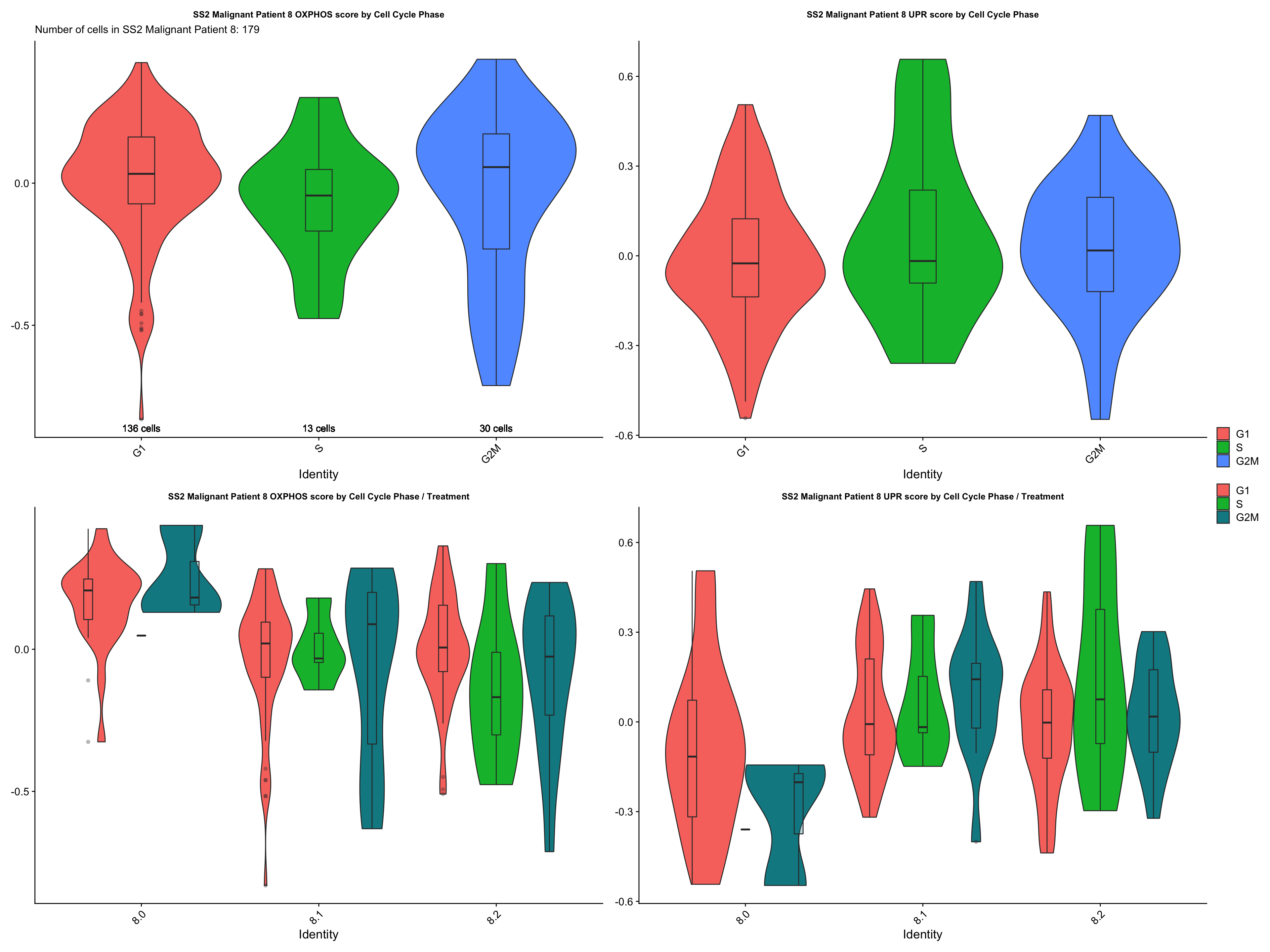

cc.exp.plot[["SS2 Malignant Patient 9"]]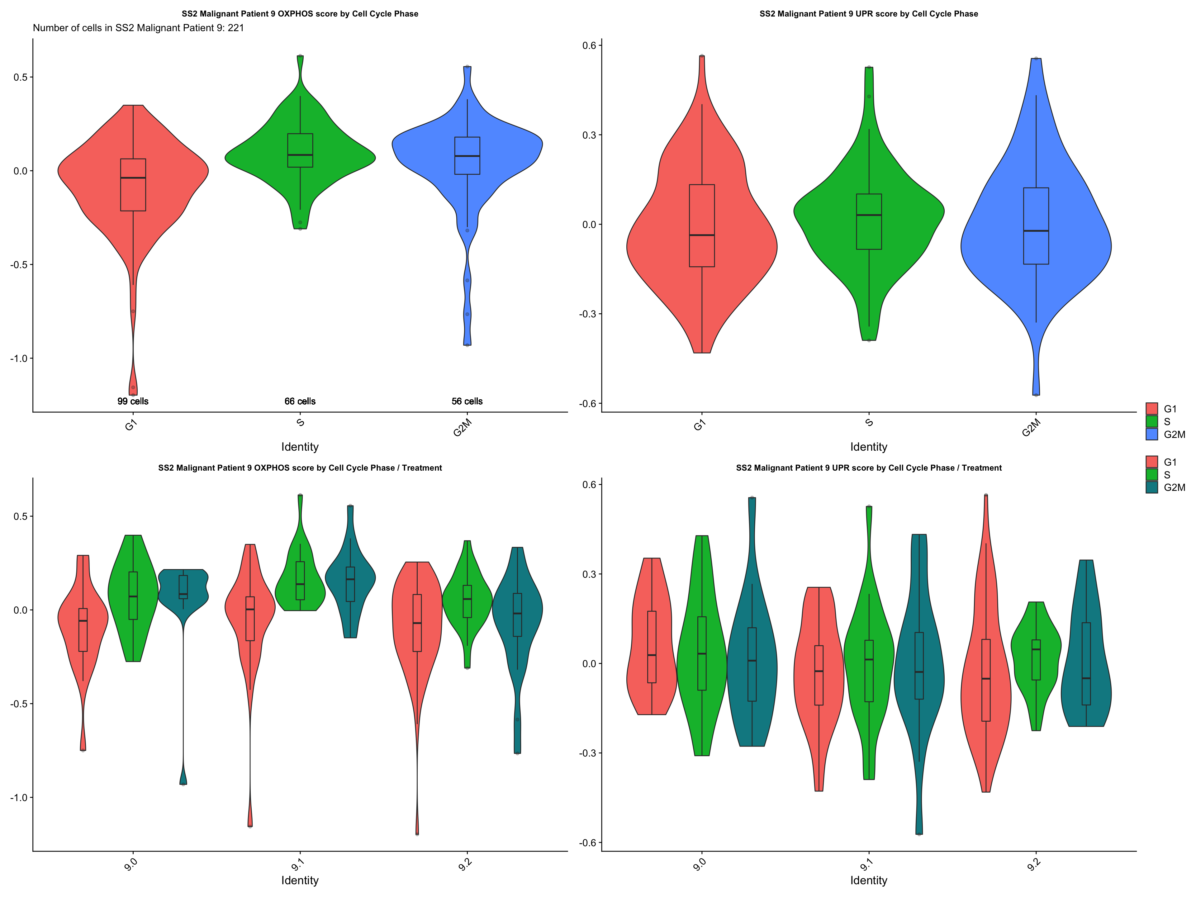

CONCLUSIONS
- Patient 8
  - OXPHOS: G2M > G1 > S (not statistically significant & does not support our hypothesis)
  - UPR: G2M > S > G1 (not statistically significant & does not support our hypothesis)
- Patient 9
  - OXPHOS: G2M > S > G1 (does not support our hypothesis)
  - UPR: S > G2M > G1 (does not support our hypothesis)
- No specific statistically significant trend identified. However, cells in the non / low cycling G1 phase do not seem to express higher levels of OXPHOS and UPR genes, which does not support our hypothesis.

sessionInfo()

R version 4.0.2 (2020-06-22)
Platform: x86_64-apple-darwin17.0 (64-bit)
Running under: macOS Mojave 10.14.6

Matrix products: default
BLAS:   /Library/Frameworks/R.framework/Versions/4.0/Resources/lib/libRblas.dylib
LAPACK: /Library/Frameworks/R.framework/Versions/4.0/Resources/lib/libRlapack.dylib

locale:
[1] en_US.UTF-8/en_US.UTF-8/en_US.UTF-8/C/en_US.UTF-8/en_US.UTF-8

attached base packages:
[1] stats     graphics  grDevices utils     datasets  methods   base     

other attached packages:
 [1] ggpubr_0.4.0          GGally_2.0.0          gt_0.2.1              reshape2_1.4.4        tidyselect_1.1.0     
 [6] presto_1.0.0          data.table_1.12.8     Rcpp_1.0.5            glue_1.4.1            patchwork_1.0.1      
[11] EnhancedVolcano_1.6.0 ggrepel_0.8.2         here_0.1              readxl_1.3.1          forcats_0.5.0        
[16] stringr_1.4.0         dplyr_1.0.0           purrr_0.3.4           readr_1.3.1           tidyr_1.1.0          
[21] tibble_3.0.3          ggplot2_3.3.2         tidyverse_1.3.0       cowplot_1.0.0         Seurat_3.1.5         
[26] BiocManager_1.30.10   renv_0.11.0-4        

loaded via a namespace (and not attached):
  [1] Rtsne_0.15         colorspace_1.4-1   ggsignif_0.6.0     rio_0.5.16         ellipsis_0.3.1     ggridges_0.5.2    
  [7] rprojroot_1.3-2    fs_1.4.2           rstudioapi_0.11    farver_2.0.3       leiden_0.3.3       listenv_0.8.0     
 [13] DT_0.14            fansi_0.4.1        lubridate_1.7.9    xml2_1.3.2         codetools_0.2-16   splines_4.0.2     
 [19] knitr_1.29         jsonlite_1.7.0     workflowr_1.6.2    broom_0.7.0        ica_1.0-2          cluster_2.1.0     
 [25] dbplyr_1.4.4       png_0.1-7          uwot_0.1.8         sctransform_0.2.1  compiler_4.0.2     httr_1.4.1        
 [31] backports_1.1.8    assertthat_0.2.1   Matrix_1.2-18      lazyeval_0.2.2     cli_2.0.2          later_1.1.0.1     
 [37] htmltools_0.5.0    tools_4.0.2        rsvd_1.0.3         igraph_1.2.5       gtable_0.3.0       RANN_2.6.1        
 [43] carData_3.0-4      cellranger_1.1.0   vctrs_0.3.2        ape_5.4            nlme_3.1-148       crosstalk_1.1.0.1 
 [49] lmtest_0.9-37      xfun_0.15          globals_0.12.5     openxlsx_4.1.5     rvest_0.3.5        lifecycle_0.2.0   
 [55] irlba_2.3.3        rstatix_0.6.0      future_1.18.0      MASS_7.3-51.6      zoo_1.8-8          scales_1.1.1      
 [61] hms_0.5.3          promises_1.1.1     parallel_4.0.2     RColorBrewer_1.1-2 curl_4.3           yaml_2.2.1        
 [67] reticulate_1.16    pbapply_1.4-2      gridExtra_2.3      reshape_0.8.8      stringi_1.4.6      zip_2.0.4         
 [73] rlang_0.4.7        pkgconfig_2.0.3    evaluate_0.14      lattice_0.20-41    ROCR_1.0-11        labeling_0.3      
 [79] htmlwidgets_1.5.1  RcppAnnoy_0.0.16   plyr_1.8.6         magrittr_1.5       R6_2.4.1           generics_0.0.2    
 [85] DBI_1.1.0          foreign_0.8-80     pillar_1.4.6       haven_2.3.1        whisker_0.4        withr_2.2.0       
 [91] fitdistrplus_1.1-1 abind_1.4-5        survival_3.2-3     future.apply_1.6.0 tsne_0.1-3         car_3.0-8         
 [97] modelr_0.1.8       crayon_1.3.4       KernSmooth_2.23-17 plotly_4.9.2.1     rmarkdown_2.3      grid_4.0.2        
[103] blob_1.2.1         git2r_0.27.1       reprex_0.3.0       digest_0.6.25      httpuv_1.5.4       munsell_0.5.0     
[109] viridisLite_0.3.0

Izar 2020 SS2 (Cohort 2) DE Analysis

Jesslyn Goh and Mike Cuoco