Simple Tree Simulations
jhmarcus
2019-04-14
Last updated: 2019-04-17
Checks: 5 1
Knit directory: drift-workflow/analysis/
This reproducible R Markdown analysis was created with workflowr (version 1.2.0). The Report tab describes the reproducibility checks that were applied when the results were created. The Past versions tab lists the development history.
The R Markdown file has unstaged changes. To know which version of the R Markdown file created these results, you’ll want to first commit it to the Git repo. If you’re still working on the analysis, you can ignore this warning. When you’re finished, you can run wflow_publish to commit the R Markdown file and build the HTML.
Great job! The global environment was empty. Objects defined in the global environment can affect the analysis in your R Markdown file in unknown ways. For reproduciblity it’s best to always run the code in an empty environment.
The command set.seed(20190211) was run prior to running the code in the R Markdown file. Setting a seed ensures that any results that rely on randomness, e.g. subsampling or permutations, are reproducible.
Great job! Recording the operating system, R version, and package versions is critical for reproducibility.
Nice! There were no cached chunks for this analysis, so you can be confident that you successfully produced the results during this run.
Great! You are using Git for version control. Tracking code development and connecting the code version to the results is critical for reproducibility. The version displayed above was the version of the Git repository at the time these results were generated.
Note that you need to be careful to ensure that all relevant files for the analysis have been committed to Git prior to generating the results (you can use wflow_publish or wflow_git_commit). workflowr only checks the R Markdown file, but you know if there are other scripts or data files that it depends on. Below is the status of the Git repository when the results were generated:
Ignored files:
    Ignored:    .Rhistory
    Ignored:    analysis/.Rhistory
    Ignored:    analysis/flash_cache/
    Ignored:    data.tar.gz
    Ignored:    data/datasets/
    Ignored:    data/raw/
    Ignored:    output.tar.gz
    Ignored:    output/

Unstaged changes:
    Modified:   analysis/simple_tree_simulation.Rmd
    Modified:   code/viz.R
Note that any generated files, e.g. HTML, png, CSS, etc., are not included in this status report because it is ok for generated content to have uncommitted changes.
These are the previous versions of the R Markdown and HTML files. If you’ve configured a remote Git repository (see ?wflow_git_remote), click on the hyperlinks in the table below to view them.
| File | Version | Author | Date | Message |
|---|---|---|---|---|
| Rmd | 1a21d43 | jhmarcus | 2019-04-17 | updated simple tree doc |
| html | 1a21d43 | jhmarcus | 2019-04-17 | updated simple tree doc |
| Rmd | 0a3374d | jhmarcus | 2019-04-15 | added simple sim |
| html | 0a3374d | jhmarcus | 2019-04-15 | added simple sim |
Introduction
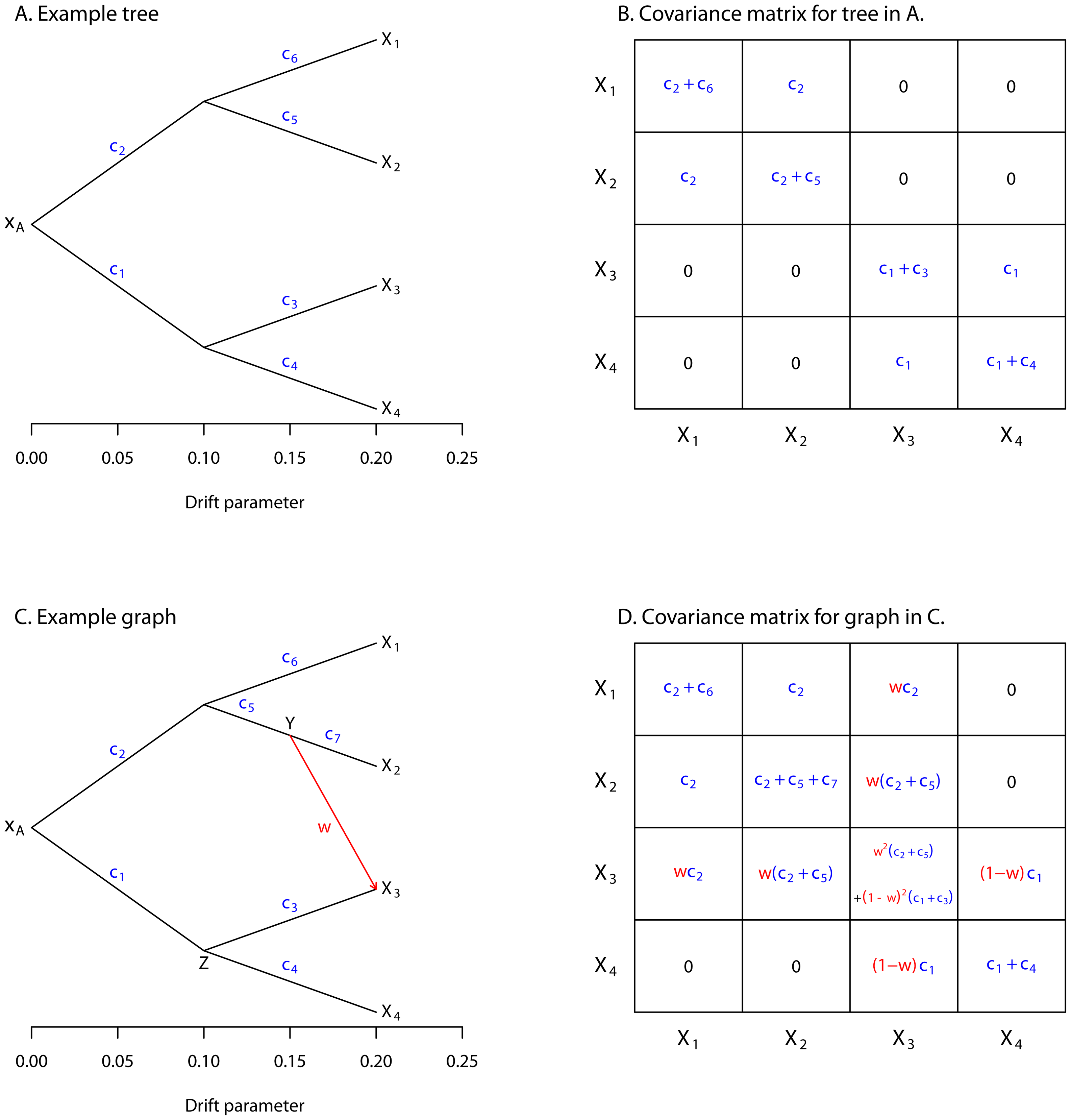
Here I explore FLASH applied to simulations under a simple population tree, as described in Pickrell et al 2012. Specifically I use a multivariate normal approximation to allele frequencies under a fixed tree and generate genotype data given these allele frequencies. See Figure 1 from Pickrell and Pritchard 2012 that shows the parameterization of the tree:
Import
Here I import the some required packages:
library(ggplot2)
library(dplyr)
library(tidyr)
library(flashier)
library(alstructure)
source("../code/nmf.R")
source("../code/viz.R")
Functions
Here are a couple functions to help with the simulations and plotting:
#' @title Simple Graph Simulation
#'
#' @description Simulates genotypes under a simple population
#'              tree as described in Pickrell and Pritchard 2012:
#'
#'              https://journals.plos.org/plosgenetics/article?id=10.1371/journal.pgen.1002967
#'
#' @param n_per_pop number of individuals per population
#' @param p number of SNPs
#' @param w admixture weight from population 2 --> 3
#' @param c1 branch length 1
#' @param c2 branch length 2
#' @param c3 branch length 3
#' @param c4 branch length 4
#' @param c5 branch length 5
#' @param c6 branch length 6
#' @param c7 branch length 7
#' @param mu_a mean allele frequency of the ancestral population
#' @sigma_e std. deviation of the allele frequency
#'          in the ancestral population
#'
#' @return list of matrix genotypes and allele frequencies
#'         allele frequencies in the ancestral population
#'
simple_graph_simulation = function(n_per_pop=10,
                                   p=1000,
                                   w=0.0,
                                   c1=.1,
                                   c2=.1,
                                   c3=.1,
                                   c4=.1,
                                   c5=.05,
                                   c6=.1,
                                   c7=.05,
                                   mu_a=.5,
                                   sigma_e=.05){

  # number of populations
  n_pops = 4

  # simulate ancestral allele freqeuncy
  p_a = mu_a + rnorm(p, 0, sigma_e)

  # ancestral variance
  sigma_a = p_a * (1.0 - p_a)

  # covariance matrix specified by the tree
  V = matrix(NA, nrow=4, ncol=4)
  V[1, 1] = c2 + c6
  V[2, 1] = V[1, 2] = c2
  V[2, 2] = c2 + c5 + c7
  V[3, 1] = V[1, 3] =  w * c2
  V[3, 2] = V[2, 3] = w * (c2 + c5)
  V[3, 3] = (w^2 * (c2 + c5)) + ((1 - w)^2 * (c1 + c3))
  V[4, 1] = V[1, 4] = 0.0
  V[4, 2] = V[2, 4] = 0.0
  V[4, 3] = V[3, 4] = (1.0 - w) * c1
  V[4, 4] = c1 + c4

  # simulate allele frequencies
  P = matrix(NA, nrow=p, ncol=n_pops)
  for(j in 1:p){

    # simulate from truncated multivariate normal
    P[j, ] = tmvtnorm::rtmvnorm(1, rep(p_a[j], n_pops), sigma_a[j] * V,
                                lower=rep(1e-4, n_pops),
                                upper=rep(1.0-1e-4, n_pops)
                                )
  }


  # simulate genotypes
  Y = matrix(rbinom(n_per_pop * p, 2, P[,1]), nrow=p, ncol=n_per_pop)
  for(i in 2:n_pops){
    Y_i = matrix(rbinom(n_per_pop * p, 2, P[,i]), nrow=p, ncol=n_per_pop)
    Y = cbind(Y, Y_i)
  }

  return(list(Y=t(Y), P=t(P), p_a=p_a))

}

plot_flash_loadings = function(flash_fit, n_per_pop){

  l_df = as.data.frame(flash_fit$loadings$normalized.loadings[[1]])
  colnames(l_df) = paste0("K", 1:ncol(l_df))
  l_df$ID = 1:nrow(l_df)
  l_df$pop = c(rep("Pop1", n_per_pop), rep("Pop2", n_per_pop),
               rep("Pop3", n_per_pop), rep("Pop4", n_per_pop))
  gath_l_df = l_df %>% gather(K, value, -ID, -pop) %>% filter(K != "K1")

  p1 = ggplot(gath_l_df, aes(x=ID, y=value, color=pop)) +
       geom_point() +
       facet_wrap(K~., scale="free") +
       theme_bw()

  p2 = structure_plot(gath_l_df,
                      colset="Set3",
                      facet_grp="pop",
                      facet_levels=paste0("Pop", 1:4),
                      fact_type="nonnegative")

  return(list(p1=p1, p2=p2))

}
Tree Simulation
Here I simulate under a tree model by setting the admixture weight \(w=0.0\). I simulate 10 individuals per population and 10,000 SNPs. I also made the branch lengths of the internal branches to be 5 times longer then the external branches.
set.seed(1990)

# number of individuals per pop
n_per_pop = 20

# set w = 0.0 to just simulate from a tree
sim = simple_graph_simulation(w=0.0, p=10000, n_per_pop=n_per_pop)

# data matrix
Y = sim$Y

# centered data matrix
Y_c = scale(Y, center=TRUE, scale=FALSE)

# centered scaled data matrix
Y_cs = scale(Y, center=TRUE, scale=TRUE)

# number of individuals
n = nrow(Y)

# number of SNPs
p = ncol(Y)

# number of factors
K = 20
PCA
Here I apply PCA to the centered and scaled genotype matrix:
svd_fit = lfa:::trunc.svd(Y_cs, K)
lamb = svd_fit$d^2
p = qplot(1:K, lamb / sum(lamb)) +
    xlab("PC") +
    ylab("PVE") +
    theme_bw()
p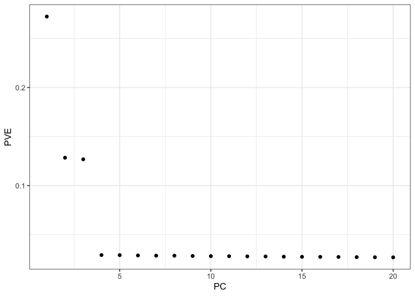
From the PVE plot we can see there is a large drop off after the first 3 PCs so lets just visualize them:
l_df = data.frame(svd_fit$u[,1:3])
colnames(l_df) = paste0("PC", 1:3)
l_df$iid = 1:n
l_df$pop = c(rep("Pop1", n_per_pop), rep("Pop2", n_per_pop),
             rep("Pop3", n_per_pop), rep("Pop4", n_per_pop))

gath_l_df = l_df %>% gather(PC, value, -iid, -pop)
p = ggplot(gath_l_df, aes(x=iid, y=value, color=pop)) +
    geom_point() +
    facet_wrap(PC~., scale="free") +
    theme_bw()
p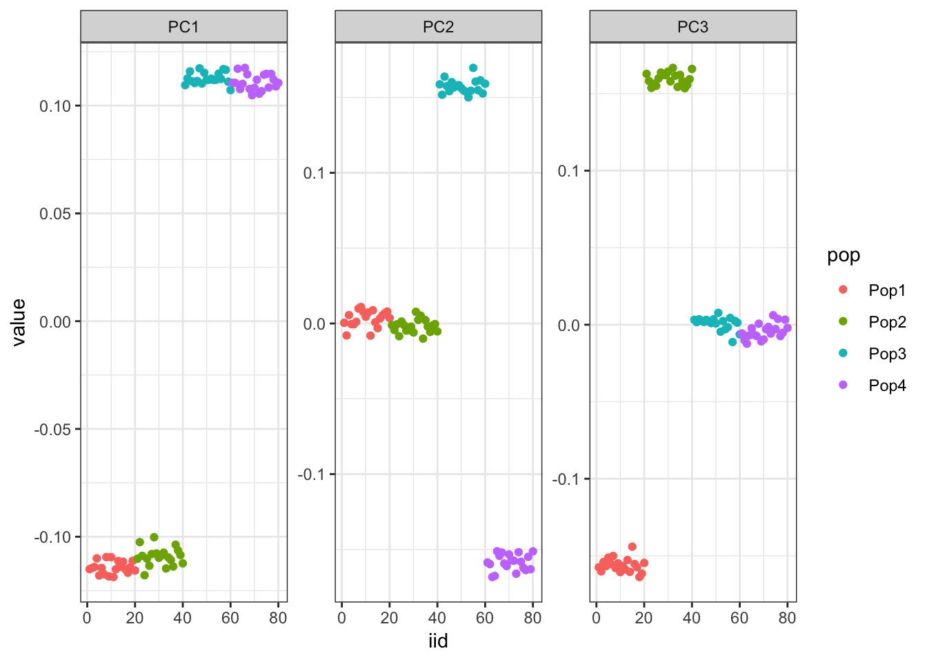
It looks like PC1 represents the first split on the tree. PC2 and PC3 represent the subsequent splits.
PSD (alstructure)
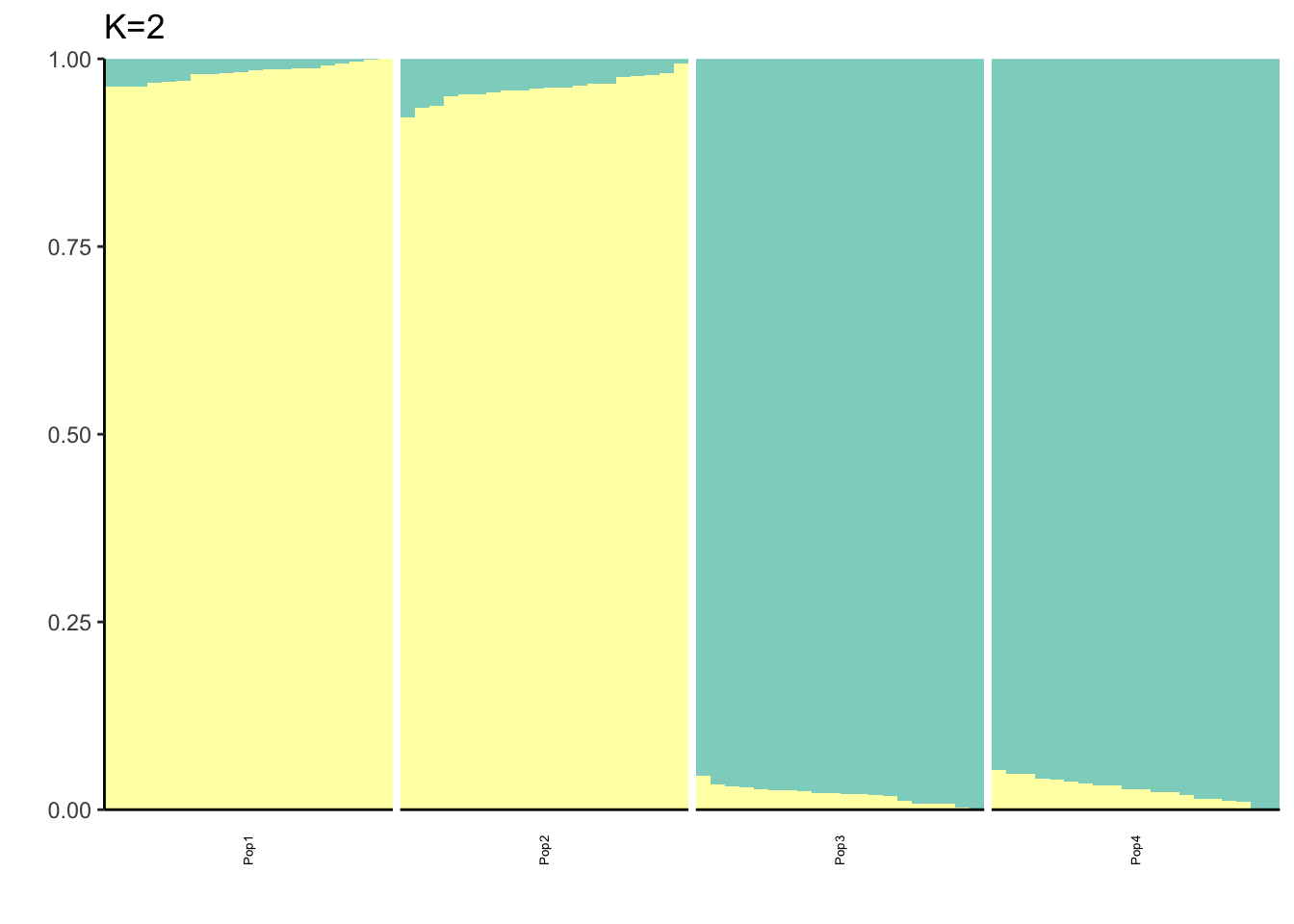
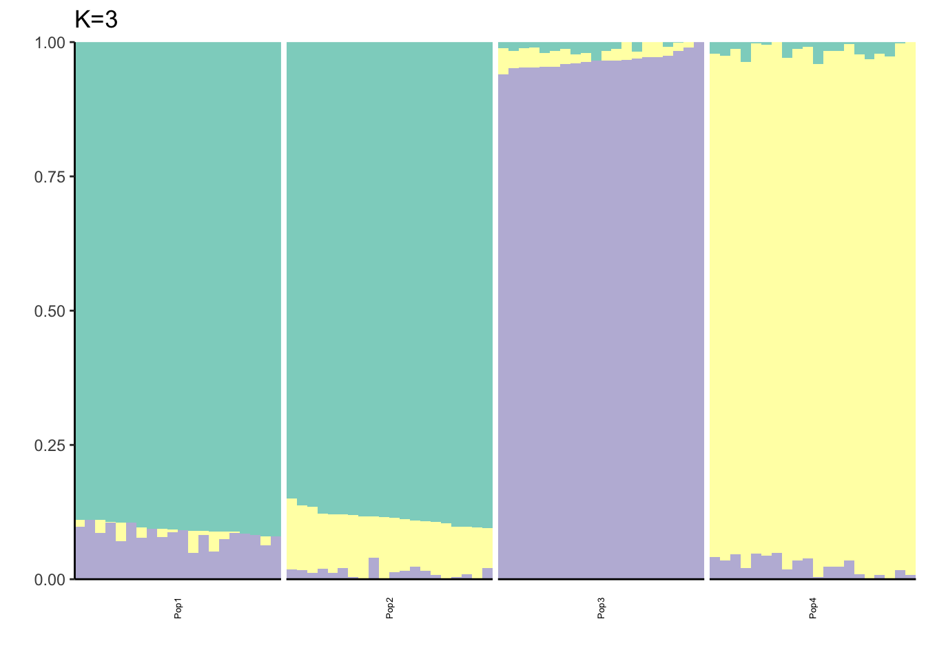
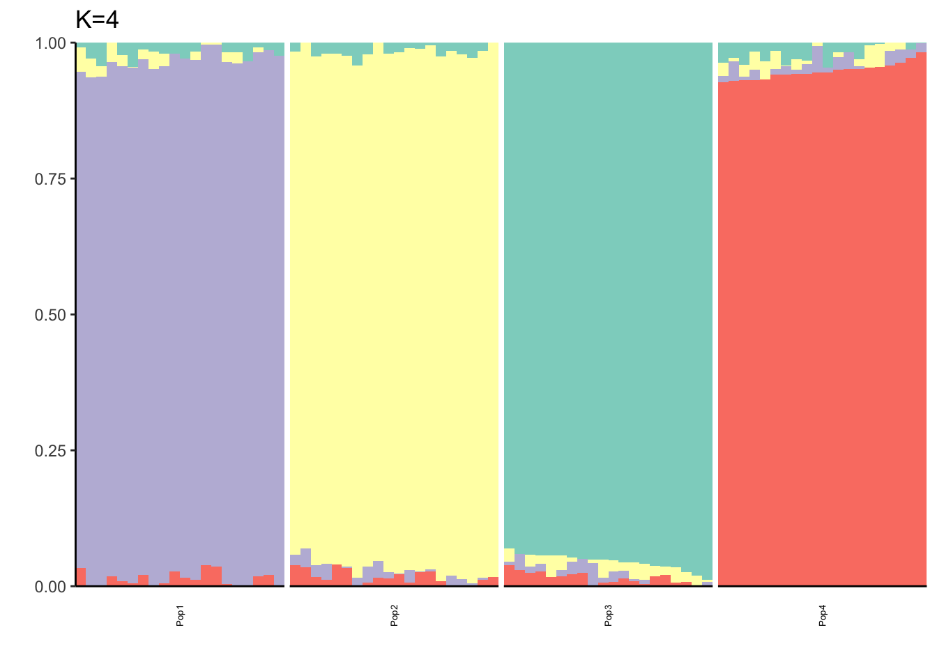
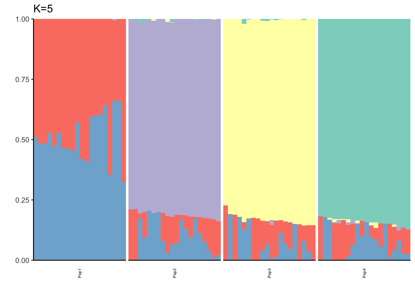
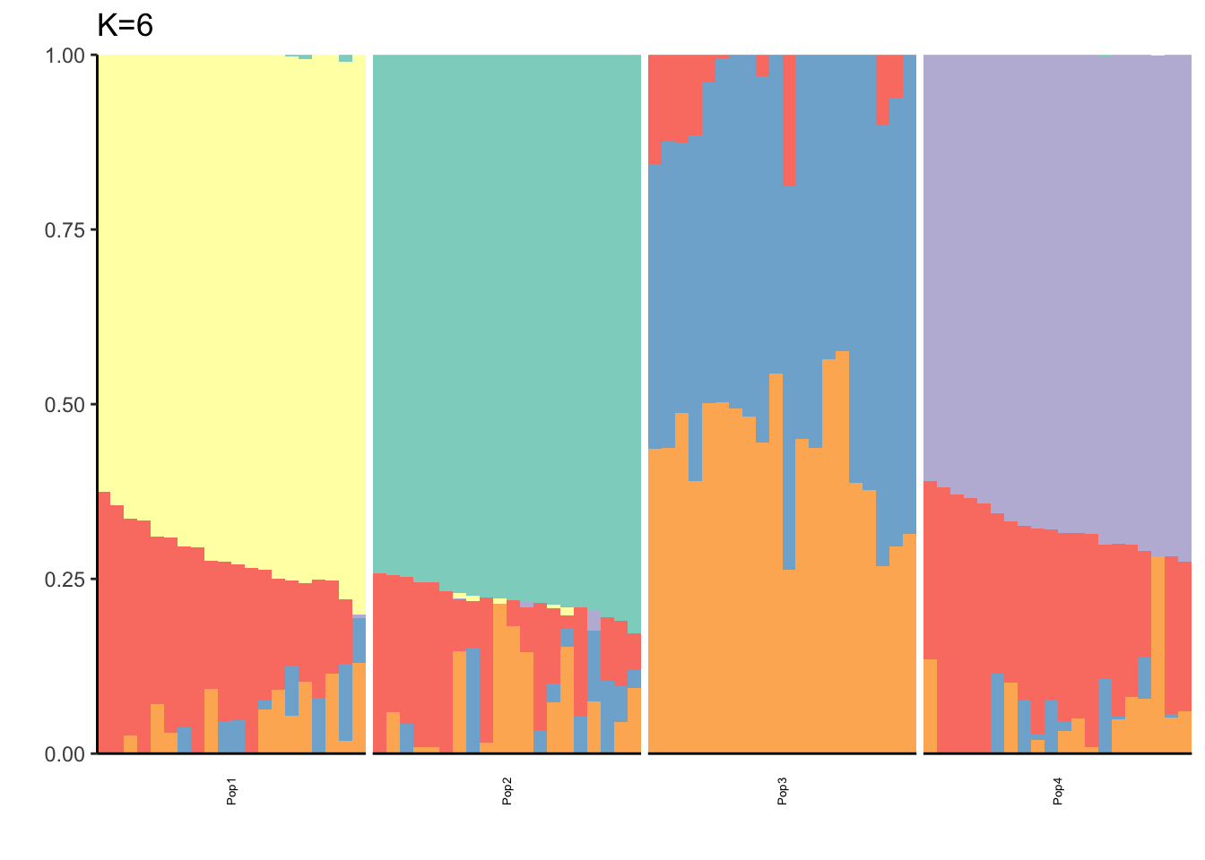
Here I fit the Pritchard, Stephens, and Donnelly model using alstructure for K=2,…,6:
K = 6
for(k in 2:K){
  al_fit = alstructure(t(Y), d_hat = k)
  Q = t(al_fit$Q_hat)
  l_df = as.data.frame(Q)
  colnames(l_df) = 1:k
  l_df$ID = 1:n
  l_df$pop = c(rep("Pop1", n_per_pop), rep("Pop2", n_per_pop),
               rep("Pop3", n_per_pop), rep("Pop4", n_per_pop))
  gath_l_df = l_df %>% gather(K, value, -ID, -pop)
  p = structure_plot(gath_l_df,
                     colset="Set3",
                     facet_grp="pop",
                     facet_levels=paste0("Pop", 1:4),
                     fact_type="structure") +
                     ggtitle(paste0("K=", k))
  print(p)
}
| Version | Author | Date |
|---|---|---|
| 1a21d43 | jhmarcus | 2019-04-17 |
| Version | Author | Date |
|---|---|---|
| 1a21d43 | jhmarcus | 2019-04-17 |
| Version | Author | Date |
|---|---|---|
| 1a21d43 | jhmarcus | 2019-04-17 |
| Version | Author | Date |
|---|---|---|
| 1a21d43 | jhmarcus | 2019-04-17 |
| Version | Author | Date |
|---|---|---|
| 1a21d43 | jhmarcus | 2019-04-17 |
It looks like for \(K=2\) we see the deeper split in the tree, \(K=4\) assigns population specific factors, and all the other K runs are less interpretable.
FLASH (Drift)
Here I apply Empirical Bayes matrix factorization with non-negative loadings and unconstrained factors. I fixed the factors to come from a normal prior with mean 0 and variance 1:
Fix Loadings Greedy
Here I fix the first loadings vector to the 1 vector and only run the greedy algorithm:
flash_fit = flashier::flashier(Y,
                               greedy.Kmax=K,
                               prior.type=c("nonnegative", "point.normal"),
                               ebnm.param=list(fixg=TRUE, g=list(pi0 = 0, a=1, mu=0)),
                               var.type=0,
                               fix.dim=list(1),
                               fix.idx=list(1:n),
                               fix.vals=list(rep(1, n)))
Initializing flash object...
Adding factor 1 to flash object...
Adding factor 2 to flash object...
Adding factor 3 to flash object...
Adding factor 4 to flash object...
Adding factor 5 to flash object...
Adding factor 6 to flash object...
Adding factor 7 to flash object...
Nullchecking 6 factors...
Wrapping up...
Done.p_res = plot_flash_loadings(flash_fit, n_per_pop)
print(p_res$p1)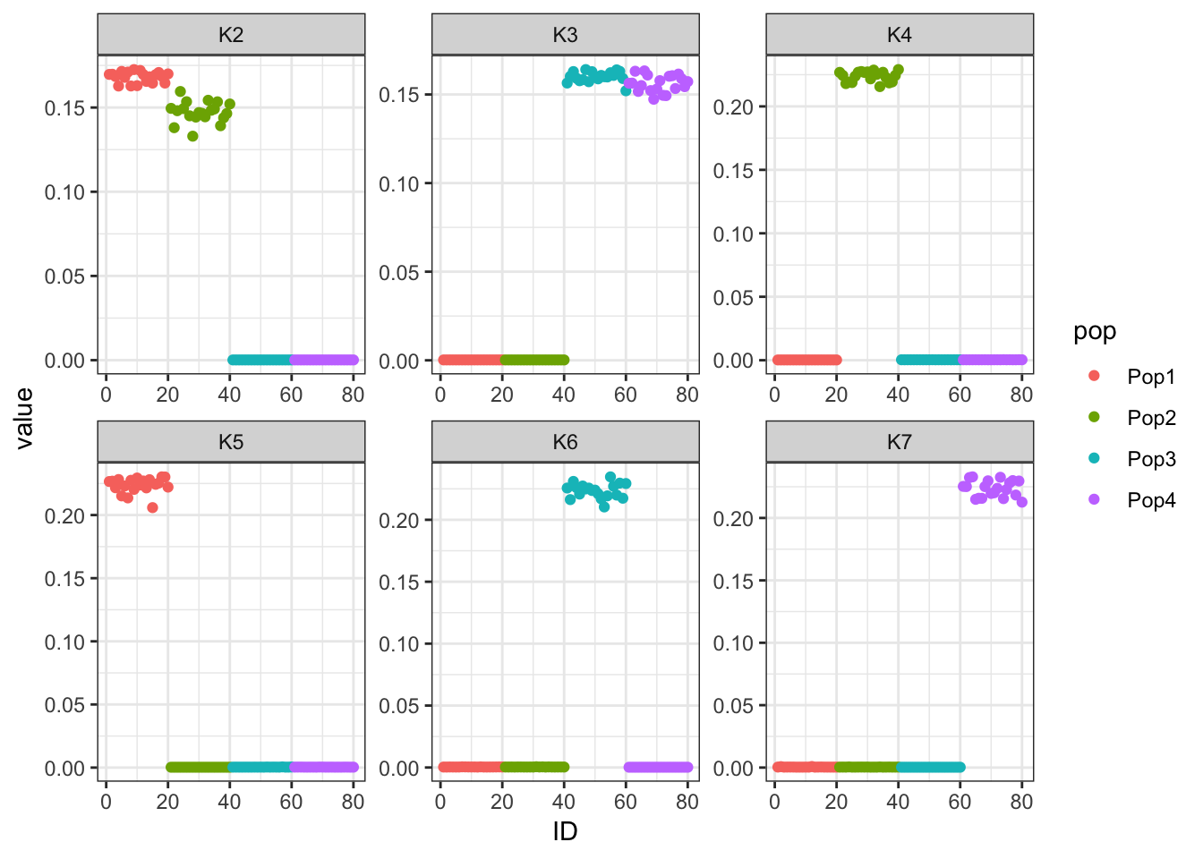
print(p_res$p2)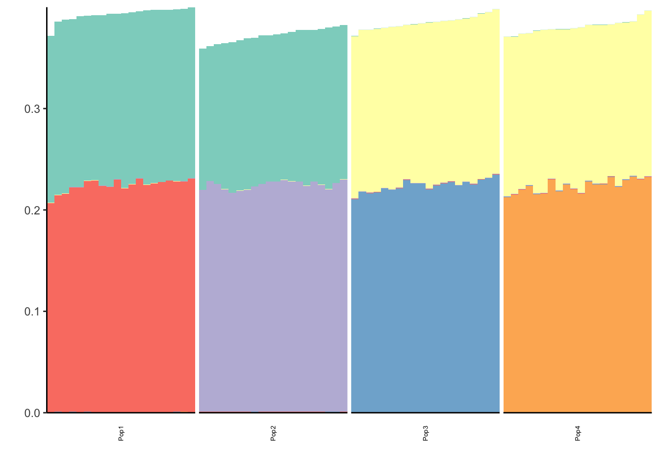
print(flash_fit$objective)[1] -863108.4Very cool … K2,K3 represent the internal nodes of the tree and K4,K5,K6,K7 represent the leaves i.e. population specific factors.
Fix Loadings Final Backfit
Here I fix the first loadings vector to the 1 vector, run the greedy algorithm to pick out \(K\) from the data and then run a final backfit to clean up the greedy solution:
flash_fit = flashier::flashier(Y,
                               flash.init = flash_fit,
                               prior.type=c("nonnegative", "point.normal"),
                               ebnm.param=list(fixg=TRUE, g=list(pi0 = 0, a=1, mu=0)),
                               var.type=0,
                               fix.dim=list(1),
                               fix.idx=list(1:n),
                               fix.vals=list(rep(1, n)),
                               backfit="final",
                               backfit.order="dropout",
                               backfit.reltol=10)
Initializing flash object...
Adding factor 8 to flash object...
Factor doesn't increase objective and won't be added.
Backfitting 7 factors...
An update to factor 7 decreased the objective by 3.531e+00.
An update to factor 2 decreased the objective by 6.613e+00.
Nullchecking 6 factors...
Factor 3 removed, increasing objective by 1.413e-01.
Factor 5 removed, increasing objective by 7.832e-02.
Adding factor 8 to flash object...
Factor doesn't increase objective and won't be added.
Backfitting 7 factors...
An update to factor 7 decreased the objective by 7.263e+00.
Nullchecking 6 factors...
Wrapping up...
Done.p_res = plot_flash_loadings(flash_fit, n_per_pop)
print(p_res$p1)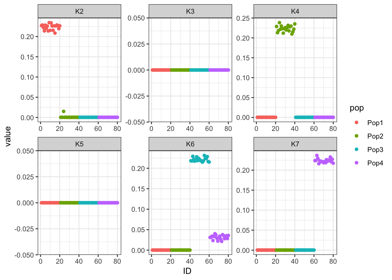
print(p_res$p2)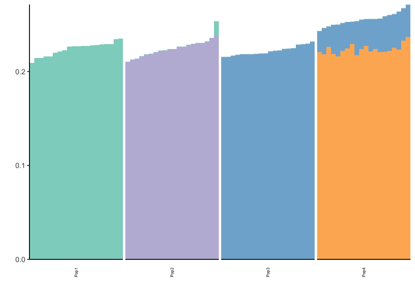
print(flash_fit$objective)[1] -851287Hmm it seems like the final backfit removes the nice signal we had in the greedy run and it zeros out some of the factors.
Fix Loadings Alternating Backfit
Here I fix the first loadings vector to the 1 vector and run a scheme where backfitting is performed after greedily adding each factor:
flash_fit = flashier::flashier(Y,
                               greedy.Kmax=K,
                               prior.type=c("nonnegative", "point.normal"),
                               ebnm.param=list(fixg=TRUE, g=list(pi0 = 0, a=1, mu=0)),
                               var.type=0,
                               fix.dim=list(1),
                               fix.idx=list(1:n),
                               fix.vals=list(rep(1, n)),
                               backfit = "alternating",
                               backfit.order = "dropout",
                               backfit.reltol = 10)
Initializing flash object...
Adding factor 1 to flash object...
Adding factor 2 to flash object...
Backfitting 2 factors...
An update to factor 2 decreased the objective by 7.768e+00.
Adding factor 3 to flash object...
Backfitting 3 factors...
Adding factor 4 to flash object...
Backfitting 4 factors...
An update to factor 3 decreased the objective by 4.801e+00.
Adding factor 5 to flash object...
Factor doesn't increase objective and won't be added.
Nullchecking 3 factors...
Wrapping up...
Done.p_res = plot_flash_loadings(flash_fit, n_per_pop)
print(p_res$p1)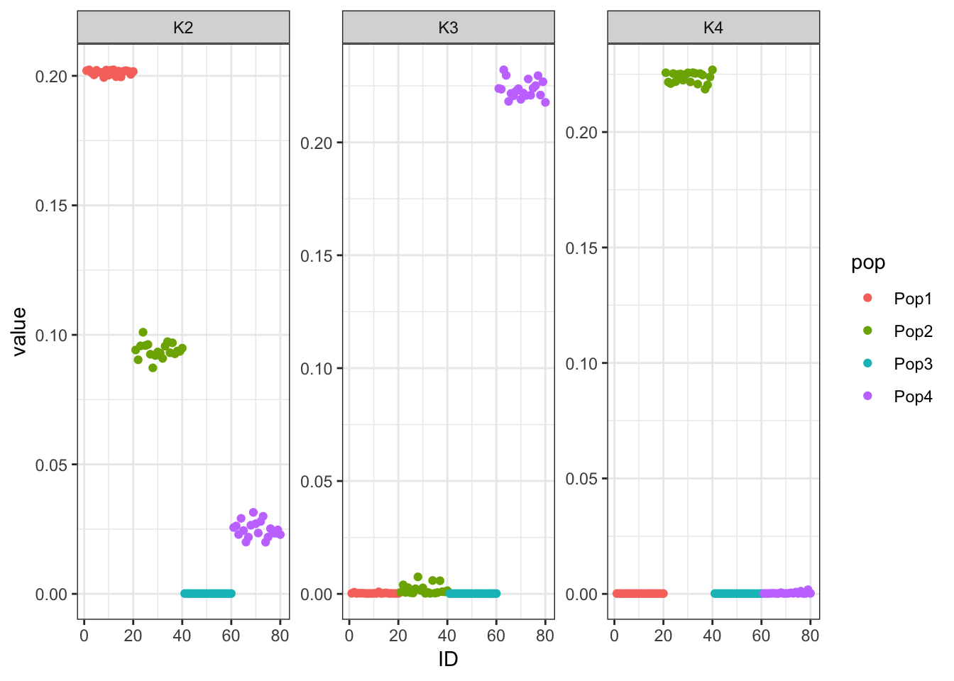
print(p_res$p2)
print(flash_fit$objective)[1] -848845.9Again this leads to an odd solution with only two population specific factors and its not obvious what K2 represents.
Mean Center Greedy
Here I don’t fix the first loadings vector and just mean center the data matrix before running greedy FLASH (Drift):
flash_fit = flashier::flashier(Y_c,
                               greedy.Kmax=K,
                               prior.type=c("nonnegative", "point.normal"),
                               ebnm.param=list(fixg=TRUE, g=list(pi0 = 0, a=1, mu=0)),
                               var.type=0)
Initializing flash object...
Adding factor 1 to flash object...
Adding factor 2 to flash object...
Adding factor 3 to flash object...
Adding factor 4 to flash object...
Adding factor 5 to flash object...
Adding factor 6 to flash object...
Nullchecking 6 factors...
Wrapping up...
Done.p_res = plot_flash_loadings(flash_fit, n_per_pop)
print(p_res$p1)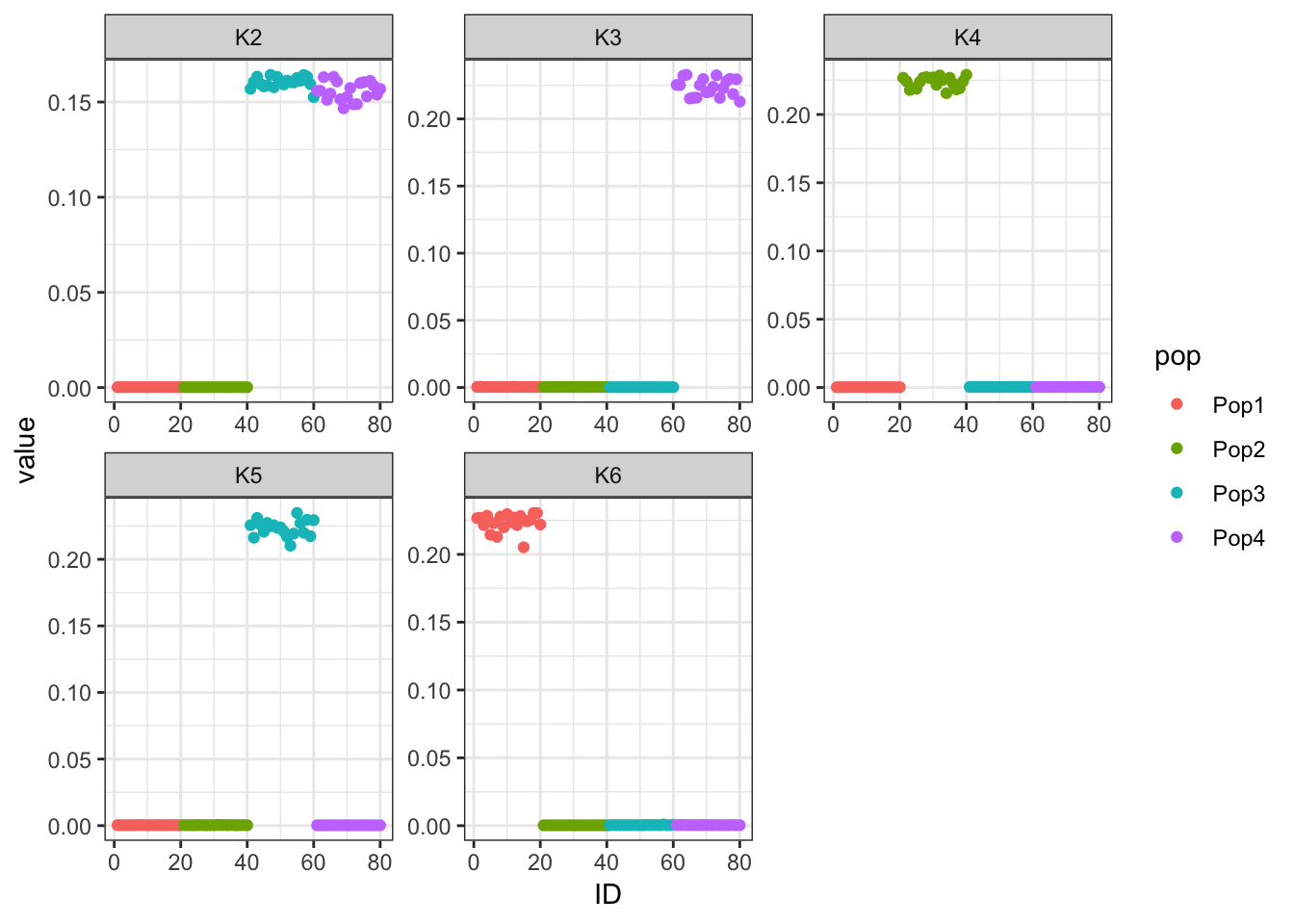
print(p_res$p2)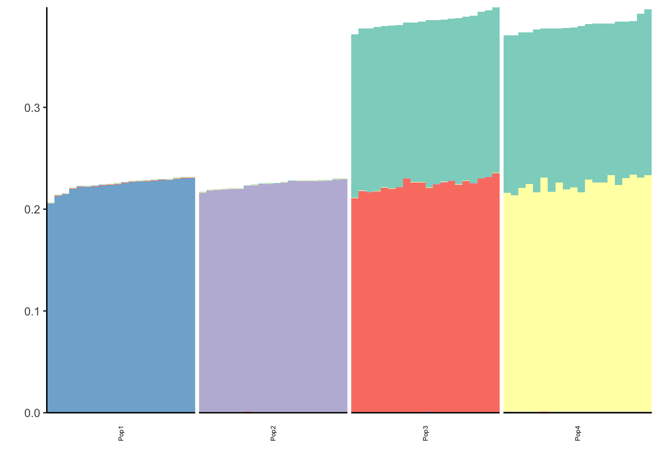
print(flash_fit$objective)[1] -831565Mean centering gives a similar solution to fixing the first factor.
Mean Center Final Backfit
Here I don’t fix the first loadings vector and just mean center the data matrix before running greedy FLASH (Drift) with a final backfit:
flash_fit = flashier::flashier(Y_c,
                               flash.init = flash_fit,
                               prior.type=c("nonnegative", "point.normal"),
                               ebnm.param=list(fixg=TRUE, g=list(pi0 = 0, a=1, mu=0)),
                               var.type=0,
                               fix.dim=list(1),
                               fix.idx=list(1:n),
                               fix.vals=list(rep(1, n)),
                               backfit="final",
                               backfit.order="dropout",
                               backfit.reltol=10)
Initializing flash object...
Adding factor 7 to flash object...
Factor doesn't increase objective and won't be added.
Backfitting 6 factors...
Nullchecking 5 factors...
Factor 2 removed, increasing objective by 1.402e-01.
Factor 6 removed, increasing objective by 7.608e-02.
Adding factor 7 to flash object...
Factor doesn't increase objective and won't be added.
Backfitting 6 factors...
Nullchecking 5 factors...
Wrapping up...
Done.p_res = plot_flash_loadings(flash_fit, n_per_pop)
print(p_res$p1)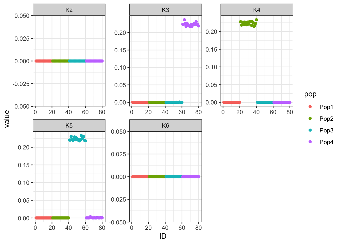
print(p_res$p2)
print(flash_fit$objective)[1] -823596.8We seem to be missing a few of the population specific factors?
Mean Center Alternating Backfit
Here I don’t fix the first loadings vector and just mean center the data matrix before running greedy FLASH (Drift) with alternating backfits:
flash_fit = flashier::flashier(Y,
                               greedy.Kmax=K,
                               prior.type=c("nonnegative", "point.normal"),
                               ebnm.param=list(fixg=TRUE, g=list(pi0 = 0, a=1, mu=0)),
                               var.type=0,
                               fix.dim=list(1),
                               fix.idx=list(1:n),
                               fix.vals=list(rep(1, n)),
                               backfit = "alternating",
                               backfit.order = "dropout",
                               backfit.reltol = 10)
Initializing flash object...
Adding factor 1 to flash object...
Adding factor 2 to flash object...
Backfitting 2 factors...
An update to factor 2 decreased the objective by 7.768e+00.
Adding factor 3 to flash object...
Backfitting 3 factors...
Adding factor 4 to flash object...
Backfitting 4 factors...
An update to factor 3 decreased the objective by 4.801e+00.
Adding factor 5 to flash object...
Factor doesn't increase objective and won't be added.
Nullchecking 3 factors...
Wrapping up...
Done.p_res = plot_flash_loadings(flash_fit, n_per_pop)
print(p_res$p1)
print(p_res$p2)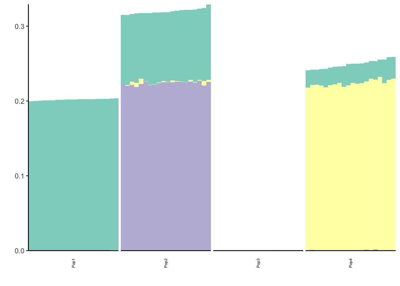
print(flash_fit$objective)[1] -848845.9Again we see only population specific factors but not shared factors.
FLASH
Here I run FLASH with no sign constraints on the loadings or factors:
Mean Center Greedy
Here I mean center the data matrix before running greedy FLASH:
flash_fit = flashier::flashier(Y_c,
                               greedy.Kmax=K,
                               prior.type=c("normal.mixture", "point.normal"),
                               ebnm.param=list(fixg=TRUE, g=list(pi0 = 0, a=1, mu=0)),
                               var.type=0)
Initializing flash object...
Adding factor 1 to flash object...
Adding factor 2 to flash object...
Adding factor 3 to flash object...
Adding factor 4 to flash object...
Factor doesn't increase objective and won't be added.
Nullchecking 3 factors...
Wrapping up...
Done.p_res = plot_flash_loadings(flash_fit, n_per_pop)
print(p_res$p1)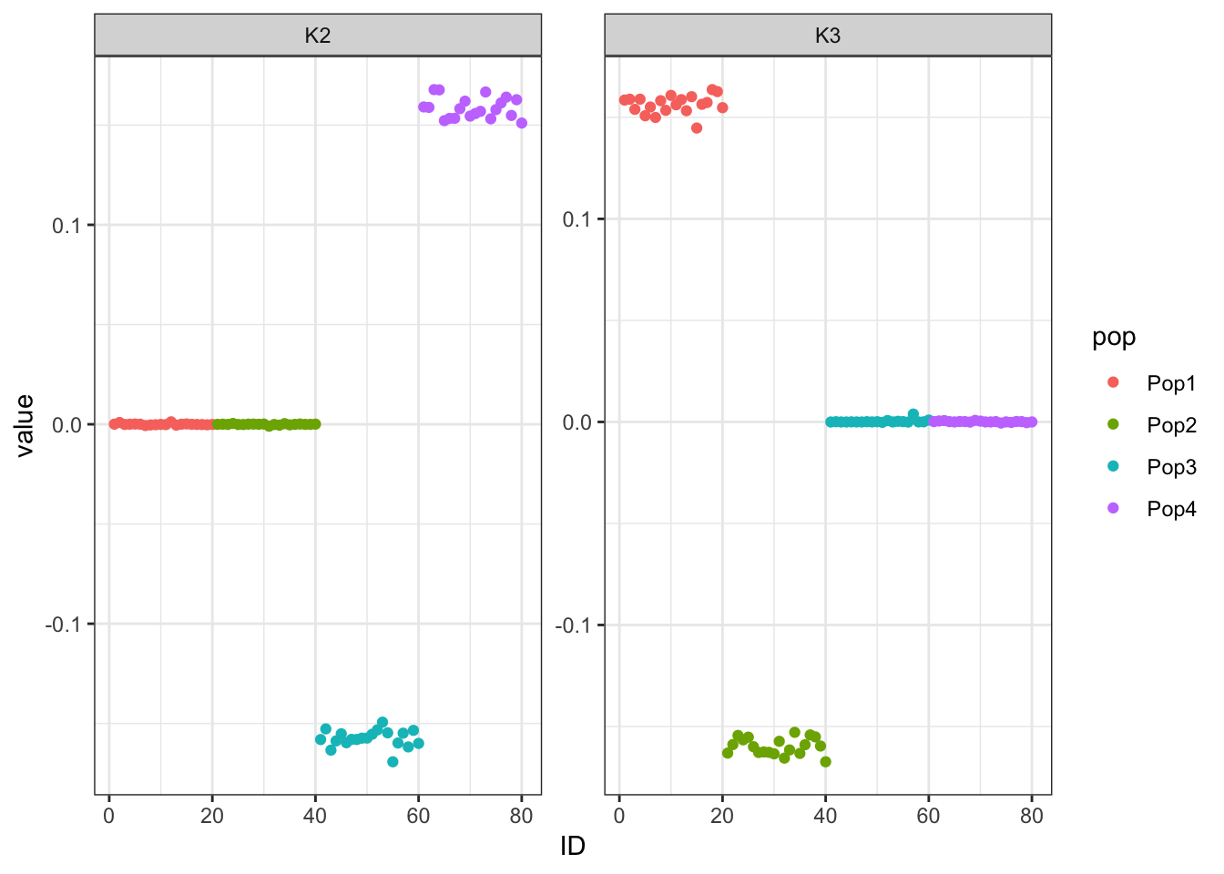
print(p_res$p2)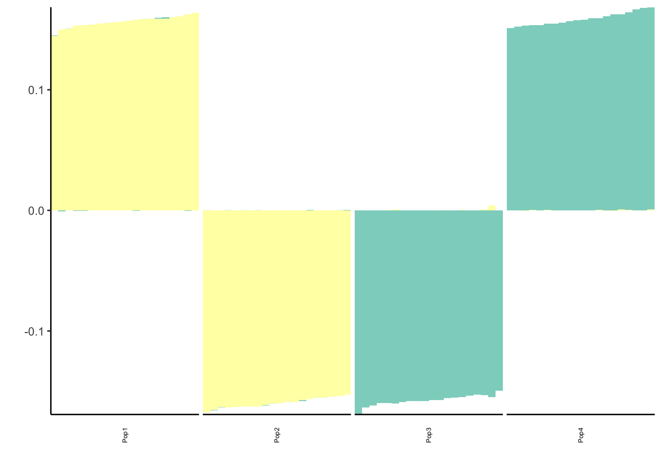
print(flash_fit$objective)[1] -809486.8Here we get a pretty nice solution similar to PCA but with a more interpretable sparsity pattern. K1 cleanly represents the first split in the tree and K2 and K3 cleanly represent the subsequent splits.
Mean Center Final Backfit
Here I mean center the data matrix before running greedy FLASH with a final backfit:
flash_fit = flashier::flashier(Y_c,
                               flash.init=flash_fit,
                               prior.type=c("normal.mixture", "point.normal"),
                               ebnm.param=list(fixg=TRUE, g=list(pi0 = 0, a=1, mu=0)),
                               var.type=0,
                               backfit = "final",
                               backfit.order = "dropout",
                               backfit.reltol = 10)
Initializing flash object...
Adding factor 4 to flash object...
Factor doesn't increase objective and won't be added.
Backfitting 3 factors...
Nullchecking 3 factors...
Wrapping up...
Done.p_res = plot_flash_loadings(flash_fit, n_per_pop)
print(p_res$p1)
print(p_res$p2)
print(flash_fit$objective)[1] -809448.4This solution looks very similar to the greedy solution.
Mean Center Alternating Backfit
Here I mean center the data matrix before running greedy FLASH with alternating backfits:
flash_fit = flashier::flashier(Y_c,
                               greedy.Kmax=K,
                               prior.type=c("normal.mixture", "point.normal"),
                               ebnm.param=list(fixg=TRUE, g=list(pi0 = 0, a=1, mu=0)),
                               var.type=0,
                               backfit = "alternating",
                               backfit.order = "dropout",
                               backfit.reltol = 10)
Initializing flash object...
Adding factor 1 to flash object...
Adding factor 2 to flash object...
Backfitting 2 factors...
Adding factor 3 to flash object...
Backfitting 3 factors...
Adding factor 4 to flash object...
Factor doesn't increase objective and won't be added.
Nullchecking 3 factors...
Wrapping up...
Done.p_res = plot_flash_loadings(flash_fit, n_per_pop)
print(p_res$p1)
print(p_res$p2)
print(flash_fit$objective)[1] -809448.3This solution also looks very similar to the greedy / final back solutions.
Convex-NMF
I implemented convex non-negative matrix factorization from Ding et al 2012 see code/nmf.R. I wanted to see if the greedy approach using another nmf algorithm would lead to a similar result to semi-negative FLASH:
Greedy
Z = t(Y)
K = 6
Znew = Z
L = matrix(NA, nrow=n, ncol=K)
for(k in 1:K){

  print(paste0("Running K=", k))
  res = convex_nmf(Znew, 1, init="kmeans", n_iter=5000, eps=1e-4, n_print=200)
  G = res$G
  F = res$F
  L[,k] = G[,1]
  Znew = Znew - res$Xhat

}
[1] "Running K=1"
[1] "iteration=200 | delta_rss=0.000214369792956859"
[1] "Running K=2"
[1] "Running K=3"
[1] "iteration=200 | delta_rss=0.000158286478836089"
[1] "Running K=4"
[1] "iteration=200 | delta_rss=0.15425558865536"
[1] "iteration=400 | delta_rss=0.0260007910546847"
[1] "iteration=600 | delta_rss=0.0150750136235729"
[1] "iteration=800 | delta_rss=0.0103306274977513"
[1] "iteration=1000 | delta_rss=0.00728529569460079"
[1] "iteration=1200 | delta_rss=0.00523876002989709"
[1] "iteration=1400 | delta_rss=0.00383262085961178"
[1] "iteration=1600 | delta_rss=0.00284782325616106"
[1] "iteration=1800 | delta_rss=0.00214615417644382"
[1] "iteration=2000 | delta_rss=0.00163837859872729"
[1] "iteration=2200 | delta_rss=0.00126567838015035"
[1] "iteration=2400 | delta_rss=0.000988550134934485"
[1] "iteration=2600 | delta_rss=0.000780007394496351"
[1] "iteration=2800 | delta_rss=0.000621327024418861"
[1] "iteration=3000 | delta_rss=0.00049933441914618"
[1] "iteration=3200 | delta_rss=0.000404637889005244"
[1] "iteration=3400 | delta_rss=0.000330461596604437"
[1] "iteration=3600 | delta_rss=0.000271862430963665"
[1] "iteration=3800 | delta_rss=0.000225196417886764"
[1] "iteration=4000 | delta_rss=0.000187751196790487"
[1] "iteration=4200 | delta_rss=0.000157488917466253"
[1] "iteration=4400 | delta_rss=0.000132865563500673"
[1] "iteration=4600 | delta_rss=0.000112701382022351"
[1] "Running K=5"
[1] "iteration=200 | delta_rss=0.00327718106564134"
[1] "iteration=400 | delta_rss=0.00257390743354335"
[1] "iteration=600 | delta_rss=0.0020490403403528"
[1] "iteration=800 | delta_rss=0.00165133021073416"
[1] "iteration=1000 | delta_rss=0.00134574202820659"
[1] "iteration=1200 | delta_rss=0.00110790698090568"
[1] "iteration=1400 | delta_rss=0.000920604856219143"
[1] "iteration=1600 | delta_rss=0.00077148579293862"
[1] "iteration=1800 | delta_rss=0.000651568523608148"
[1] "iteration=2000 | delta_rss=0.000554236699827015"
[1] "iteration=2200 | delta_rss=0.000474555941764265"
[1] "iteration=2400 | delta_rss=0.000408804742619395"
[1] "iteration=2600 | delta_rss=0.000354146060999483"
[1] "iteration=2800 | delta_rss=0.000308395712636411"
[1] "iteration=3000 | delta_rss=0.000269856071099639"
[1] "iteration=3200 | delta_rss=0.000237196451053023"
[1] "iteration=3400 | delta_rss=0.000209364865440875"
[1] "iteration=3600 | delta_rss=0.000185523473192006"
[1] "iteration=3800 | delta_rss=0.000164999801199883"
[1] "iteration=4000 | delta_rss=0.000147250830195844"
[1] "iteration=4200 | delta_rss=0.000131834880448878"
[1] "iteration=4400 | delta_rss=0.000118390482384712"
[1] "iteration=4600 | delta_rss=0.000106620485894382"
[1] "Running K=6"
[1] "iteration=200 | delta_rss=0.00080844247713685"
[1] "iteration=400 | delta_rss=0.000725734047591686"
[1] "iteration=600 | delta_rss=0.000652785762213171"
[1] "iteration=800 | delta_rss=0.000588317634537816"
[1] "iteration=1000 | delta_rss=0.000531231053173542"
[1] "iteration=1200 | delta_rss=0.000480581889860332"
[1] "iteration=1400 | delta_rss=0.000435557274613529"
[1] "iteration=1600 | delta_rss=0.000395456328988075"
[1] "iteration=1800 | delta_rss=0.000359673576895148"
[1] "iteration=2000 | delta_rss=0.000327685207594186"
[1] "iteration=2200 | delta_rss=0.000299037026707083"
[1] "iteration=2400 | delta_rss=0.000273334793746471"
[1] "iteration=2600 | delta_rss=0.000250235374551266"
[1] "iteration=2800 | delta_rss=0.000229439756367356"
[1] "iteration=3000 | delta_rss=0.000210686994250864"
[1] "iteration=3200 | delta_rss=0.000193748681340367"
[1] "iteration=3400 | delta_rss=0.000178424816112965"
[1] "iteration=3600 | delta_rss=0.000164539844263345"
[1] "iteration=3800 | delta_rss=0.000151939457282424"
[1] "iteration=4000 | delta_rss=0.000140487623866647"
[1] "iteration=4200 | delta_rss=0.000130064552649856"
[1] "iteration=4400 | delta_rss=0.000120564131066203"
[1] "iteration=4600 | delta_rss=0.00011189270298928"
[1] "iteration=4800 | delta_rss=0.000103967089671642"l_df = data.frame(L)
colnames(l_df) = paste0("K", 1:K)
l_df$iid = 1:n
l_df$pop = c(rep("Pop1", n_per_pop), rep("Pop2", n_per_pop),
rep("Pop3", n_per_pop), rep("Pop4", n_per_pop))
gath_l_df = l_df %>% gather(K, value, -iid, -pop)
p = ggplot(gath_l_df, aes(x=iid, y=value, color=pop)) +
geom_point() +
facet_wrap(K~., scale="free") +
theme_bw()
print(p)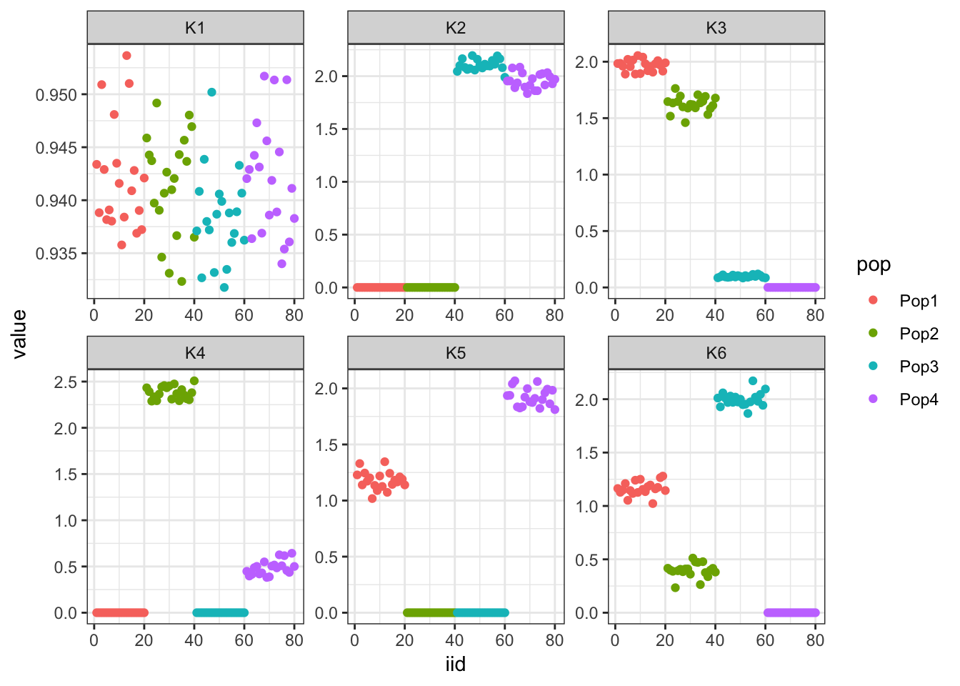
| Version | Author | Date |
|---|---|---|
| 1a21d43 | jhmarcus | 2019-04-17 |
The first factor looks like the mean then the following two look similar to greedy FLASH. The following 3 are less interpretable.
Greedy (remove ancestral mean)
Z = t(Y) - (2*sim$p_a)
K = 6
Znew = Z
L = matrix(NA, nrow=n, ncol=K)
for(k in 1:K){

  print(paste0("Running K=", k))
  res = convex_nmf(Znew, 1, init="kmeans", n_iter=5000, eps=1e-4, n_print=200)
  G = res$G
  F = res$F
  L[,k] = G[,1]
  Znew = Znew - res$Xhat

}
[1] "Running K=1"
[1] "iteration=200 | delta_rss=2.36968607478775"
[1] "iteration=400 | delta_rss=0.0060401774244383"
[1] "Running K=2"
[1] "iteration=200 | delta_rss=0.00163709180196747"
[1] "iteration=400 | delta_rss=0.000119189149700105"
[1] "Running K=3"
[1] "iteration=200 | delta_rss=0.04010079219006"
[1] "iteration=400 | delta_rss=0.0202493721735664"
[1] "iteration=600 | delta_rss=0.0143762896186672"
[1] "iteration=800 | delta_rss=0.0110623084474355"
[1] "iteration=1000 | delta_rss=0.00925089360680431"
[1] "iteration=1200 | delta_rss=0.0130199669511057"
[1] "iteration=1400 | delta_rss=0.00450576079310849"
[1] "iteration=1600 | delta_rss=0.00477232271805406"
[1] "iteration=1800 | delta_rss=0.0017393262241967"
[1] "iteration=2000 | delta_rss=0.00260783830890432"
[1] "iteration=2200 | delta_rss=0.00664551596855745"
[1] "iteration=2400 | delta_rss=0.00521458004368469"
[1] "iteration=2600 | delta_rss=0.00119250547140837"
[1] "iteration=2800 | delta_rss=0.00106901105027646"
[1] "iteration=3000 | delta_rss=0.003095222346019"
[1] "iteration=3200 | delta_rss=0.0031730595510453"
[1] "iteration=3400 | delta_rss=0.00107647129334509"
[1] "iteration=3600 | delta_rss=0.0020170253701508"
[1] "iteration=3800 | delta_rss=0.00611454120371491"
[1] "iteration=4000 | delta_rss=0.00127147982129827"
[1] "iteration=4200 | delta_rss=0.000384099257644266"
[1] "iteration=4400 | delta_rss=0.000260173401329666"
[1] "iteration=4600 | delta_rss=0.000228660472203046"
[1] "iteration=4800 | delta_rss=0.000226207368541509"
[1] "iteration=5000 | delta_rss=0.000741485739126801"
[1] "Running K=4"
[1] "iteration=200 | delta_rss=0.0571316437562928"
[1] "Running K=5"
[1] "Running K=6"
[1] "iteration=200 | delta_rss=0.00926272809738293"
[1] "iteration=400 | delta_rss=0.000970086606685072"
[1] "iteration=600 | delta_rss=0.000281919375993311"
[1] "iteration=800 | delta_rss=0.000139113748446107"l_df = data.frame(L)
colnames(l_df) = paste0("K", 1:K)
l_df$iid = 1:n
l_df$pop = c(rep("Pop1", n_per_pop), rep("Pop2", n_per_pop),
rep("Pop3", n_per_pop), rep("Pop4", n_per_pop))
gath_l_df = l_df %>% gather(K, value, -iid, -pop)
p = ggplot(gath_l_df, aes(x=iid, y=value, color=pop)) +
geom_point() +
facet_wrap(K~., scale="free") +
theme_bw()
print(p)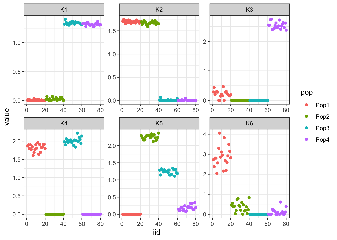
| Version | Author | Date |
|---|---|---|
| 1a21d43 | jhmarcus | 2019-04-17 |
This has a similar solution to greedy semi-negative FLASH except the first factor is way less sparse and the other factors are less sparse in general. This makes it clear how important it is to estimate the mean parameter in the model correctly.
Admixture Graph Simulation (in progress)
Here I simulate under an admixture event on the tree from population 2 to population 3 by setting the admixture weight \(w=0.4\). I simulate 10 individuals per population and 10,000 SNPs:
set.seed(1990)

# number of individuals per pop
n_per_pop = 20

# set w = 0.0 to just simulate from a tree
sim = simple_graph_simulation(w=0.4, c1=.5, c2=.5, p=10000, n_per_pop=n_per_pop)

# data matrix
Y = sim$Y

# centered data matrix
Y_c = scale(Y, center=TRUE, scale=FALSE)

# centered scaled data matrix
Y_cs = scale(Y, center=TRUE, scale=TRUE)

# number of individuals
n = nrow(Y)

# number of SNPs
p = ncol(Y)

# number of factors
K = 20
PCA
Here I apply PCA to the centered and scaled genotype matrix:
svd_fit = lfa:::trunc.svd(Y_cs, K)
lamb = svd_fit$d^2
p = qplot(1:K, lamb / sum(lamb)) +
    xlab("PC") +
    ylab("PVE") +
    theme_bw()

print(p)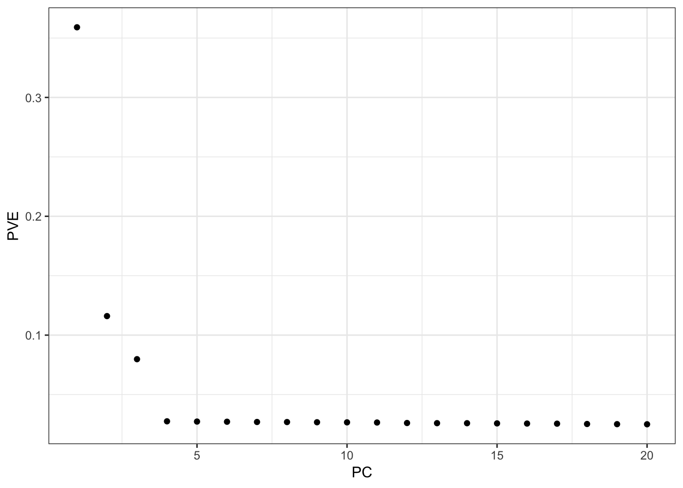
| Version | Author | Date |
|---|---|---|
| 1a21d43 | jhmarcus | 2019-04-17 |
From the PVE plot we can see there is a large drop off after the first 3 PCs so lets just visualize them:
l_df = data.frame(svd_fit$u[,1:3])
colnames(l_df) = paste0("PC", 1:3)
l_df$iid = 1:n
l_df$pop = c(rep("Pop1", n_per_pop), rep("Pop2", n_per_pop),
             rep("Pop3", n_per_pop), rep("Pop4", n_per_pop))

gath_l_df = l_df %>% gather(PC, value, -iid, -pop)
p = ggplot(gath_l_df, aes(x=iid, y=value, color=pop)) +
    geom_point() +
    facet_wrap(PC~., scale="free") +
    theme_bw()

print(p)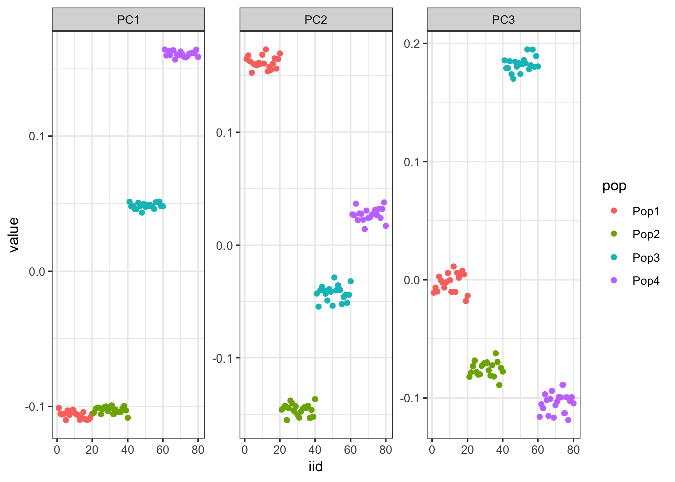
| Version | Author | Date |
|---|---|---|
| 1a21d43 | jhmarcus | 2019-04-17 |
There is some signal of the admixture event in PC1 … we see a shift of population 2 to 0.0 in PC1 rather than being cluster with population 4.
PSD (alstructure)
Here I fit the Pritchard, Stephens, and Donnelly model using alstructure for K=2,…,6:
K = 6
for(k in 2:K){
  al_fit = alstructure(t(Y), d_hat = k)
  Q = t(al_fit$Q_hat)
  l_df = as.data.frame(Q)
  colnames(l_df) = 1:k
  l_df$ID = 1:n
  l_df$pop = c(rep("Pop1", n_per_pop), rep("Pop2", n_per_pop),
               rep("Pop3", n_per_pop), rep("Pop4", n_per_pop))
  gath_l_df = l_df %>% gather(K, value, -ID, -pop)
  p = structure_plot(gath_l_df,
                     colset="Set3",
                     facet_grp="pop",
                     facet_levels=paste0("Pop", 1:4),
                     fact_type="structure") +
                     ggtitle(paste0("K=", k))

  print(p)
}
| Version | Author | Date |
|---|---|---|
| 1a21d43 | jhmarcus | 2019-04-17 |
| Version | Author | Date |
|---|---|---|
| 1a21d43 | jhmarcus | 2019-04-17 |
| Version | Author | Date |
|---|---|---|
| 1a21d43 | jhmarcus | 2019-04-17 |
| Version | Author | Date |
|---|---|---|
| 1a21d43 | jhmarcus | 2019-04-17 |
| Version | Author | Date |
|---|---|---|
| 1a21d43 | jhmarcus | 2019-04-17 |
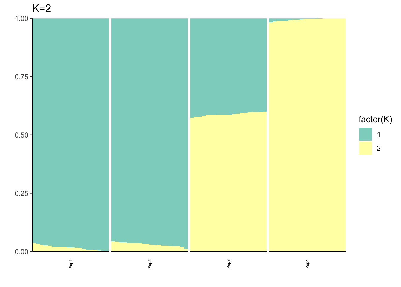
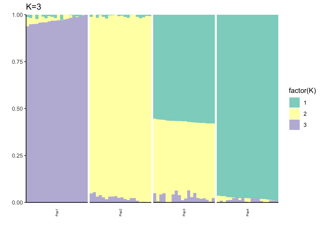
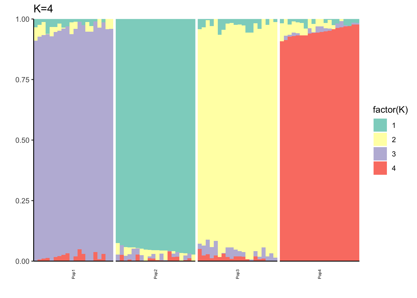
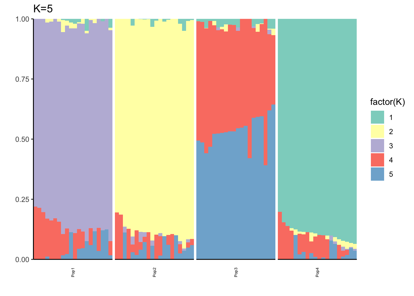
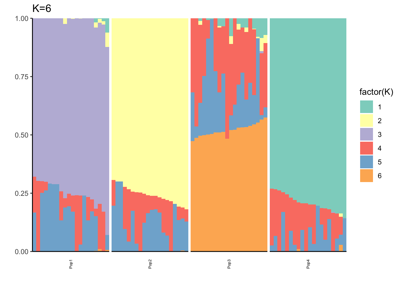
Here maybe \(K=3\) is the most interpretable? We see some signature of the split and admixture? This is already showing the difficulty of interpreting PSD fits in simple population genetic model. It also emphasizes thats the admixture gallery of many K plots needs to be shown to really understand what is going on not just a single one.
FLASH (Drift)
Here I apply Empirical Bayes matrix factorization with non-negative loadings and unconstrained factors:
Fix Loadings Greedy
Here I fix the first loadings vector to the 1 vector and only run the greedy algorithm:
flash_fit = flashier::flashier(Y,
                               greedy.Kmax=K,
                               prior.type=c("nonnegative", "point.normal"),
                               ebnm.param=list(fixg=TRUE, g=list(pi0 = 0, a=1, mu=0)),
                               var.type=0,
                               fix.dim=list(1),
                               fix.idx=list(1:n),
                               fix.vals=list(rep(1, n)))
Initializing flash object...
Adding factor 1 to flash object...
Adding factor 2 to flash object...
Adding factor 3 to flash object...
Adding factor 4 to flash object...
Adding factor 5 to flash object...
Adding factor 6 to flash object...
Adding factor 7 to flash object...
Factor doesn't increase objective and won't be added.
Nullchecking 5 factors...
Wrapping up...
Done.p_res = plot_flash_loadings(flash_fit, n_per_pop)
print(p_res$p1)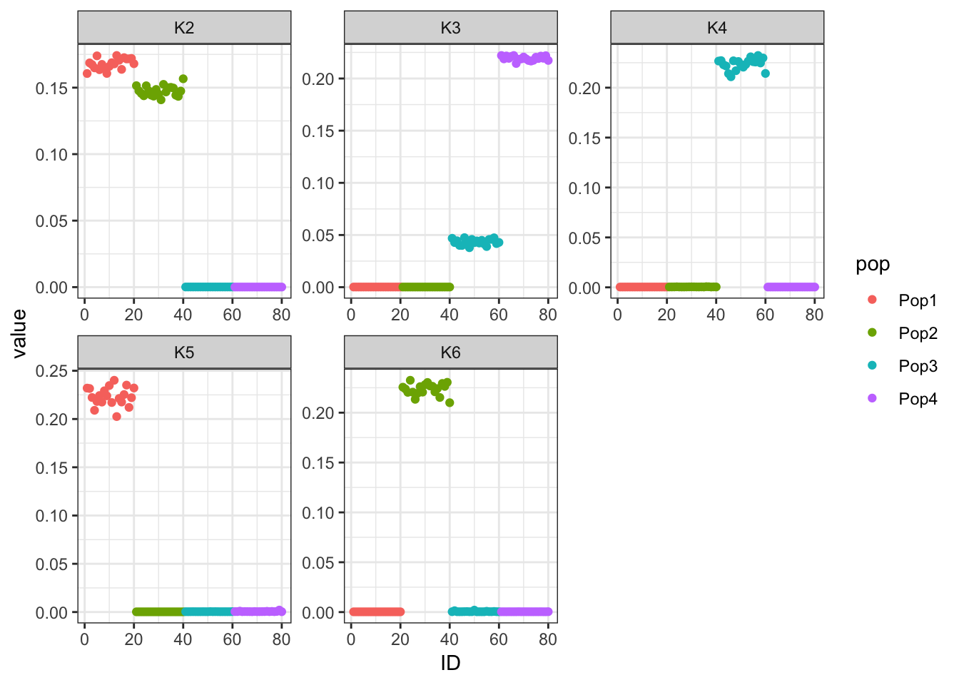
| Version | Author | Date |
|---|---|---|
| 1a21d43 | jhmarcus | 2019-04-17 |
print(p_res$p2)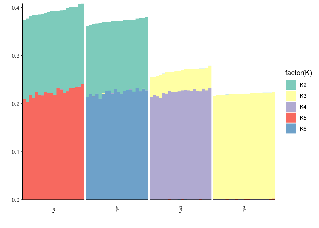
print(flash_fit$objective)[1] -832532.2Hmm we are missing the population specific factor for population 4? We also see population 3 not being as strongly loaded on factor 3 which maybe is a signature of the admixture event?
Fix Loadings Final Backfit
Here I fix the first loadings vector to the 1 vector, run the greedy algorithm to pick out \(K\) from the data and then run a final backfit to clean up the greedy solution:
flash_fit = flashier::flashier(Y,
                               flash.init = flash_fit,
                               prior.type=c("nonnegative", "point.normal"),
                               ebnm.param=list(fixg=TRUE, g=list(pi0 = 0, a=1, mu=0)),
                               var.type=0,
                               fix.dim=list(1),
                               fix.idx=list(1:n),
                               fix.vals=list(rep(1, n)),
                               backfit="final",
                               backfit.order="dropout",
                               backfit.reltol=10)
Initializing flash object...
Adding factor 7 to flash object...
Factor doesn't increase objective and won't be added.
Backfitting 6 factors...
Nullchecking 5 factors...
Factor 4 removed, increasing objective by 5.117e+00.
Factor 5 removed, increasing objective by 8.135e-02.
Adding factor 7 to flash object...
Factor doesn't increase objective and won't be added.
Backfitting 6 factors...
Nullchecking 5 factors...
Wrapping up...
Done.p_res = plot_flash_loadings(flash_fit, n_per_pop)
print(p_res$p1)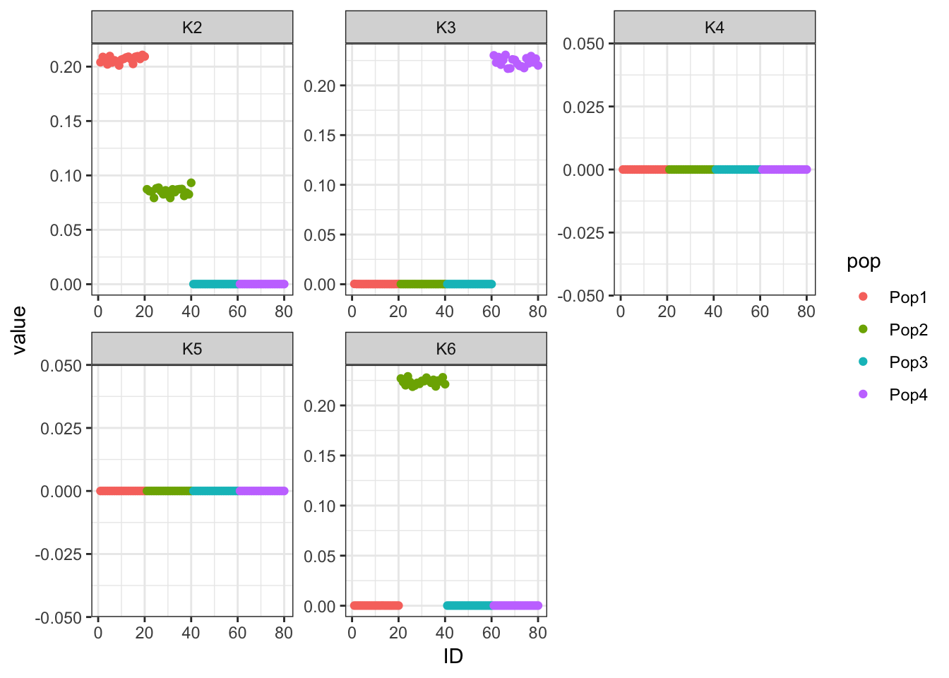
| Version | Author | Date |
|---|---|---|
| 1a21d43 | jhmarcus | 2019-04-17 |
print(p_res$p2)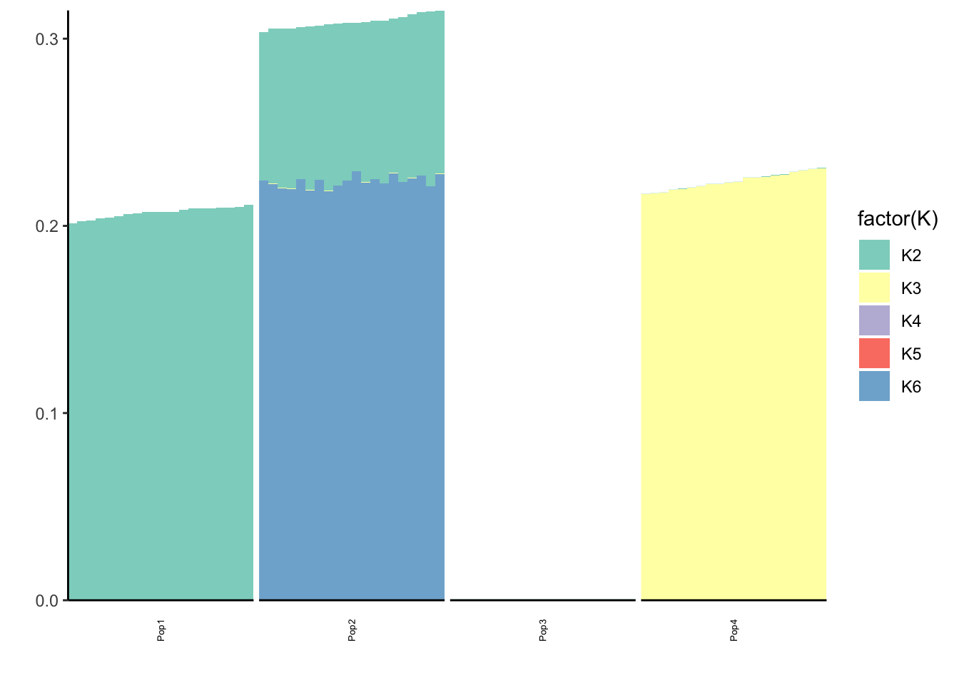
print(flash_fit$objective)[1] -821414.6This is not very interpretable.
Fix Loadings Alternating Backfit
Here I fix the first loadings vector to the 1 vector and run a scheme where backfitting is performed after greedily adding each factor:
flash_fit = flashier::flashier(Y,
                               greedy.Kmax=K,
                               prior.type=c("nonnegative", "point.normal"),
                               ebnm.param=list(fixg=TRUE, g=list(pi0 = 0, a=1, mu=0)),
                               var.type=0,
                               fix.dim=list(1),
                               fix.idx=list(1:n),
                               fix.vals=list(rep(1, n)),
                               backfit = "alternating",
                               backfit.order = "dropout",
                               backfit.reltol = 10)
Initializing flash object...
Adding factor 1 to flash object...
Adding factor 2 to flash object...
Backfitting 2 factors...
Adding factor 3 to flash object...
Backfitting 3 factors...
An update to factor 3 decreased the objective by 2.473e+00.
Adding factor 4 to flash object...
Backfitting 4 factors...
An update to factor 3 decreased the objective by 1.644e+00.
Adding factor 5 to flash object...
Factor doesn't increase objective and won't be added.
Nullchecking 3 factors...
Wrapping up...
Done.p_res = plot_flash_loadings(flash_fit, n_per_pop)
print(p_res$p1)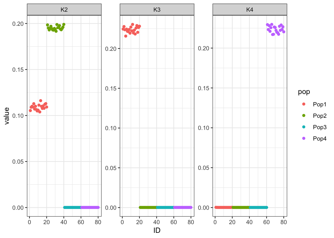
| Version | Author | Date |
|---|---|---|
| 1a21d43 | jhmarcus | 2019-04-17 |
print(p_res$p2)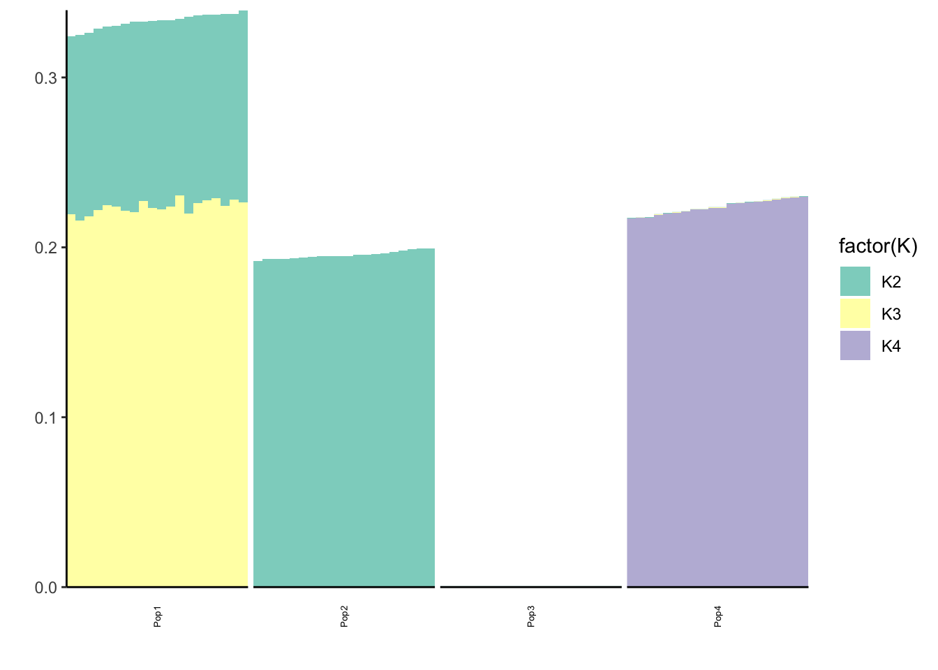
print(flash_fit$objective)[1] -821709.7
sessionInfo()R version 3.5.1 (2018-07-02)
Platform: x86_64-apple-darwin13.4.0 (64-bit)
Running under: macOS 10.14.2
Matrix products: default
BLAS/LAPACK: /Users/jhmarcus/miniconda3/lib/R/lib/libRblas.dylib
locale:
[1] en_US.UTF-8/en_US.UTF-8/en_US.UTF-8/C/en_US.UTF-8/en_US.UTF-8
attached base packages:
[1] stats graphics grDevices utils datasets methods base
other attached packages:
[1] RColorBrewer_1.1-2 alstructure_0.1.0 flashier_0.1.1
[4] tidyr_0.8.2 dplyr_0.8.0.1 ggplot2_3.1.0
loaded via a namespace (and not attached):
[1] zoo_1.8-4 tidyselect_0.2.5 xfun_0.4
[4] purrr_0.3.0 reshape2_1.4.3 ashr_2.2-35
[7] lattice_0.20-38 gmm_1.6-2 colorspace_1.4-0
[10] htmltools_0.3.6 stats4_3.5.1 yaml_2.2.0
[13] rlang_0.3.1 mixsqp_0.1-109 pillar_1.3.1
[16] glue_1.3.0 withr_2.1.2 foreach_1.4.4
[19] plyr_1.8.4 stringr_1.4.0 munsell_0.5.0
[22] gtable_0.2.0 workflowr_1.2.0 mvtnorm_1.0-10
[25] lfa_1.12.0 codetools_0.2-16 evaluate_0.12
[28] labeling_0.3 knitr_1.21 pscl_1.5.2
[31] doParallel_1.0.14 parallel_3.5.1 Rcpp_1.0.0
[34] corpcor_1.6.9 scales_1.0.0 backports_1.1.3
[37] tmvtnorm_1.4-10 truncnorm_1.0-8 fs_1.2.6
[40] digest_0.6.18 stringi_1.2.4 ebnm_0.1-17
[43] grid_3.5.1 rprojroot_1.3-2 tools_3.5.1
[46] sandwich_2.5-1 magrittr_1.5 lazyeval_0.2.1
[49] tibble_2.0.1 crayon_1.3.4 whisker_0.3-2
[52] pkgconfig_2.0.2 MASS_7.3-51.1 Matrix_1.2-15
[55] SQUAREM_2017.10-1 assertthat_0.2.0 rmarkdown_1.11
[58] iterators_1.0.10 R6_2.4.0 git2r_0.23.0
[61] compiler_3.5.1