Imports

Import the required libraries and scripts:

suppressMessages({
  library(lfa)
  library(flashier)
  library(drift.alpha)
  library(ggplot2)
  library(reshape2)
  library(tidyverse)
  library(alstructure)
})

Data

data_path <- "../output/simulations/OutOfAfrica_2T12/rep1.txt"
Y <- t(as.matrix(read.table(data_path, sep=" ")))
n <- nrow(Y)
maf <- colSums(Y) / (2 * n)

# filter out too rare and too common SNPs
Y <- Y[,((maf>=.05) & (maf <=.95))]
p <- ncol(Y)
Z <- scale(Y)
print(n)

[1] 80

print(p)

[1] 35925

# sub-population labels from stdpop
labs <- rep(c("AFR", "EUR"), each=40)

we end up with 80 individuals and ~35925 SNPs.

PCA

Lets run PCA on the centered and scaled genotype matrix:

svd_res <- lfa:::trunc.svd(Z, 5)
L_hat <- svd_res$u
plot_loadings(L_hat, labs)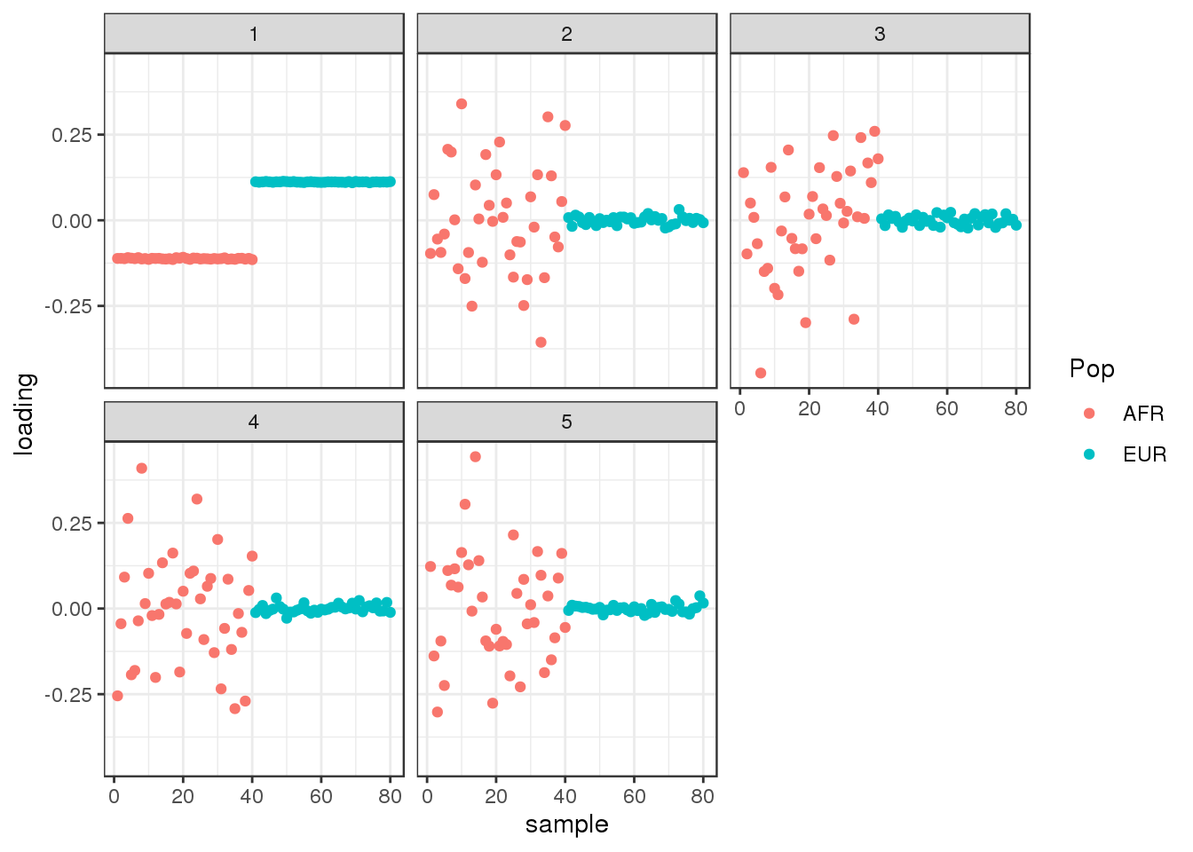

plot the first two factors against each other:

qplot(L_hat[,1], L_hat[,2], color=labs) + 
  xlab("PC1") + 
  ylab("PC2") + 
  theme_bw()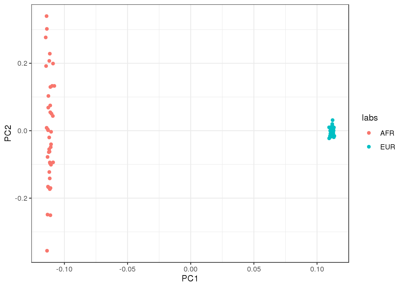

PC1 represents “Out of Africa” and PC2 represents within Africa variation.

ALStructure

Run ALStructure with \(K=2\):

admix_res <- alstructure::alstructure(t(Y), d_hat=2)
Qhat <- t(admix_res$Q_hat)
plot_loadings(Qhat, labs)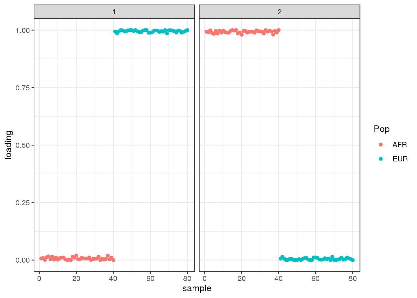

the PSD model assigns two distinct clusters.

flash [greedy]

Run the greedy algorithm:

fl <- flash(Y, 
            greedy.Kmax=5, 
            prior.family=c(prior.bimodal(), prior.normal()))

Adding factor 1 to flash object...
Adding factor 2 to flash object...
Adding factor 3 to flash object...
Adding factor 4 to flash object...
Factor doesn't significantly increase objective and won't be added.
Wrapping up...
Done.
Nullchecking 3 factors...
Done.

plot_loadings(fl$flash.fit$EF[[1]], labs)

the greedy algorithm learns a shared factor and then finds two population specific factors.

flash [backfit]

Run flash [backfit] initializing from the greedy solution:

flbf <- fl %>% 
  flash.backfit() %>% 
  flash.nullcheck(remove=TRUE)

Backfitting 3 factors (tolerance: 4.28e-02)...
  Difference between iterations is within 1.0e+02...
  Difference between iterations is within 1.0e+01...
  Difference between iterations is within 1.0e+00...
  Difference between iterations is within 1.0e-01...
Wrapping up...
Done.
Nullchecking 3 factors...
Wrapping up...
Done.

plot_loadings(flbf$flash.fit$EF[[1]], labs)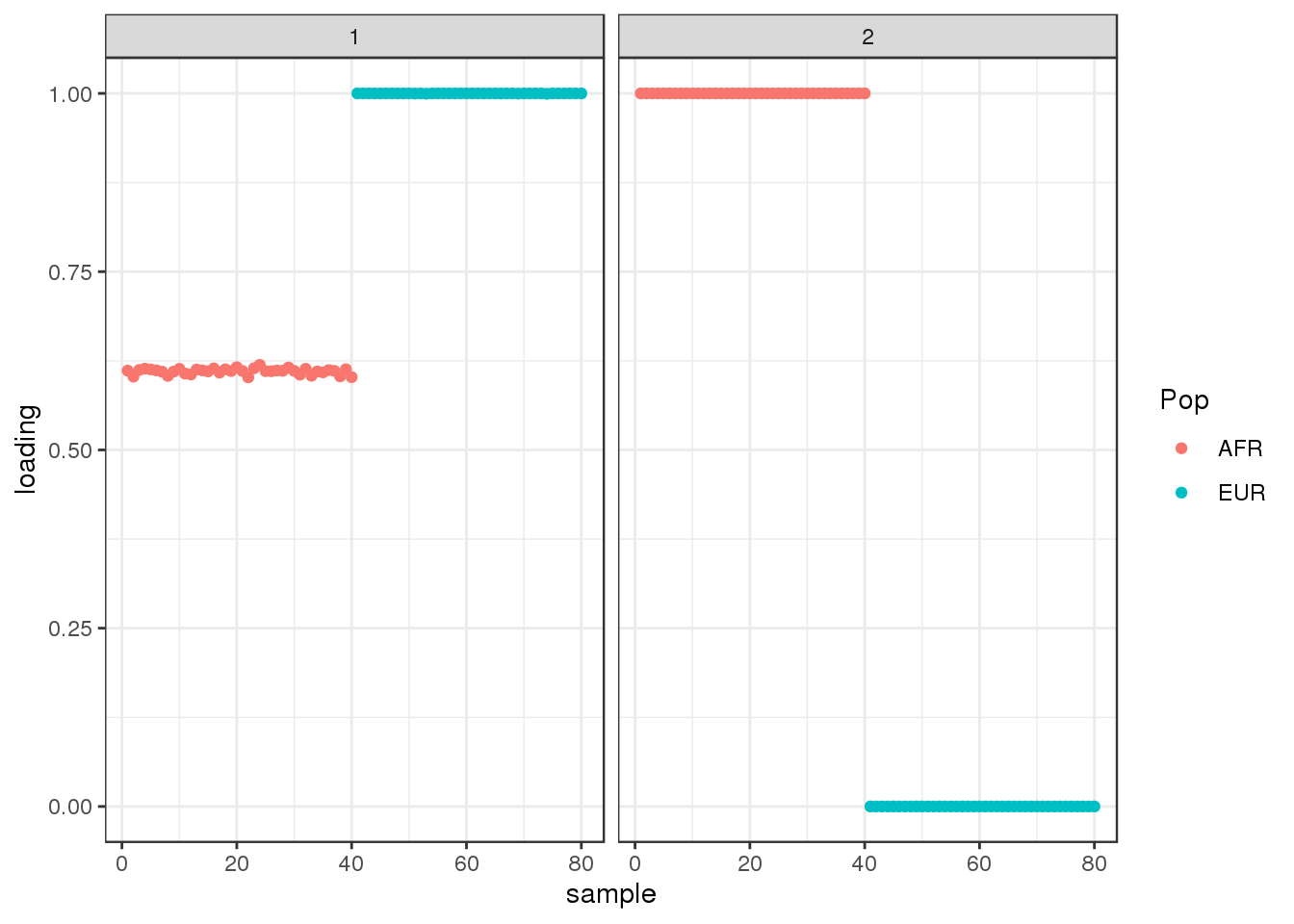

interestingly, flash finds the sparse representation of the the two population tree that we have seen before.

drift

Run drift initializing from the greedy solution:

init <- init_from_flash(fl)
dr <- drift(init, miniter=2, maxiter=500, tol=0.01, verbose=TRUE)

   1 :    -2312309.293 
   2 :    -2310400.853 
   3 :    -2310030.016 
   4 :    -2309946.385 
   5 :    -2309916.972 
   6 :    -2309899.156 
   7 :    -2309885.123 
   8 :    -2309873.347 
   9 :    -2309863.424 
  10 :    -2309855.130 
  11 :    -2309848.251 
  12 :    -2309842.565 
  13 :    -2309837.852 
  14 :    -2309833.914 
  15 :    -2309830.579 
  16 :    -2309827.663 
  17 :    -2309824.947 
  18 :    -2309822.390 
  19 :    -2309819.965 
  20 :    -2309817.645 
  21 :    -2309815.482 
  22 :    -2309813.664 
  23 :    -2309812.136 
  24 :    -2309810.853 
  25 :    -2309809.779 
  26 :    -2309808.880 
  27 :    -2309808.129 
  28 :    -2309807.502 
  29 :    -2309806.979 
  30 :    -2309806.544 
  31 :    -2309806.182 
  32 :    -2309805.882 
  33 :    -2309805.632 
  34 :    -2309805.425 
  35 :    -2309805.253 
  36 :    -2309805.110 
  37 :    -2309804.992 
  38 :    -2309804.895 
  39 :    -2309804.814 
  40 :    -2309804.747 
  41 :    -2309804.692 
  42 :    -2309804.646 
  43 :    -2309804.608 
  44 :    -2309804.577 
  45 :    -2309804.551 
  46 :    -2309804.530 
  47 :    -2309804.512 
  48 :    -2309804.498 
  49 :    -2309804.486 
  50 :    -2309804.476 

plot_loadings(dr$EL, labs)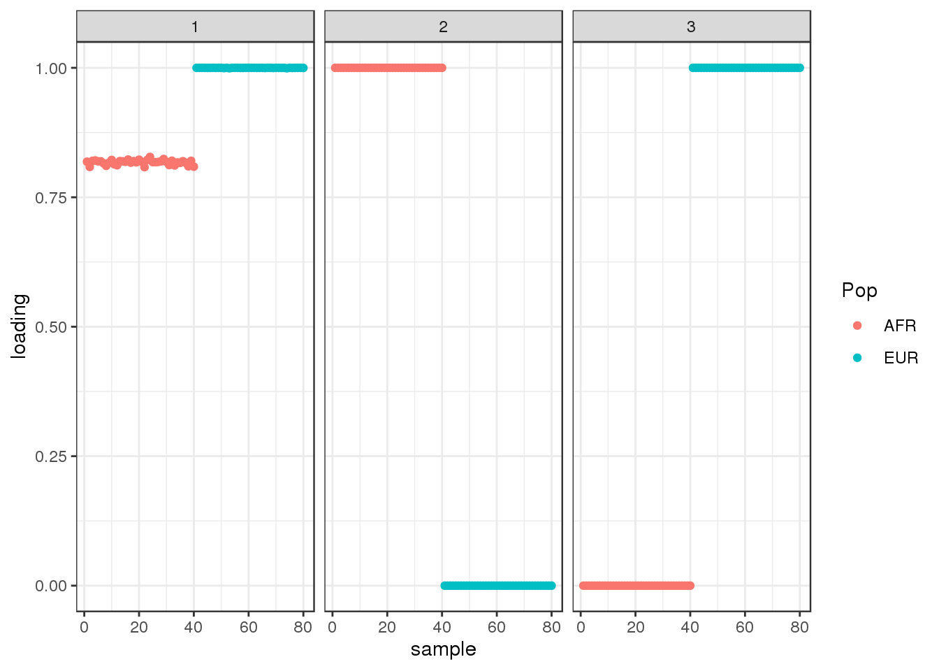

drift looks similar to the greedy algorithm.

Session information

sessionInfo()

R version 3.5.1 (2018-07-02)
Platform: x86_64-pc-linux-gnu (64-bit)
Running under: Scientific Linux 7.4 (Nitrogen)

Matrix products: default
BLAS/LAPACK: /software/openblas-0.2.19-el7-x86_64/lib/libopenblas_haswellp-r0.2.19.so

locale:
 [1] LC_CTYPE=en_US.UTF-8       LC_NUMERIC=C              
 [3] LC_TIME=en_US.UTF-8        LC_COLLATE=en_US.UTF-8    
 [5] LC_MONETARY=en_US.UTF-8    LC_MESSAGES=en_US.UTF-8   
 [7] LC_PAPER=en_US.UTF-8       LC_NAME=C                 
 [9] LC_ADDRESS=C               LC_TELEPHONE=C            
[11] LC_MEASUREMENT=en_US.UTF-8 LC_IDENTIFICATION=C       

attached base packages:
[1] stats     graphics  grDevices utils     datasets  methods   base     

other attached packages:
 [1] alstructure_0.1.0 forcats_0.5.0     stringr_1.4.0    
 [4] dplyr_0.8.5       purrr_0.3.4       readr_1.3.1      
 [7] tidyr_1.0.2       tibble_3.0.1      tidyverse_1.3.0  
[10] reshape2_1.4.3    ggplot2_3.3.0     drift.alpha_0.0.9
[13] flashier_0.2.4    lfa_1.9.0        

loaded via a namespace (and not attached):
 [1] httr_1.4.1       jsonlite_1.6     modelr_0.1.6     assertthat_0.2.1
 [5] mixsqp_0.3-17    cellranger_1.1.0 yaml_2.2.0       ebnm_0.1-24     
 [9] pillar_1.4.3     backports_1.1.6  lattice_0.20-38  glue_1.4.0      
[13] digest_0.6.25    promises_1.0.1   rvest_0.3.5      colorspace_1.4-1
[17] htmltools_0.3.6  httpuv_1.4.5     Matrix_1.2-15    plyr_1.8.4      
[21] pkgconfig_2.0.3  invgamma_1.1     broom_0.5.6      haven_2.2.0     
[25] corpcor_1.6.9    scales_1.1.0     whisker_0.3-2    later_0.7.5     
[29] git2r_0.26.1     farver_2.0.3     generics_0.0.2   ellipsis_0.3.0  
[33] withr_2.2.0      ashr_2.2-50      cli_2.0.2        magrittr_1.5    
[37] crayon_1.3.4     readxl_1.3.1     evaluate_0.14    fs_1.3.1        
[41] fansi_0.4.1      nlme_3.1-137     xml2_1.3.2       truncnorm_1.0-8 
[45] tools_3.5.1      hms_0.5.3        lifecycle_0.2.0  munsell_0.5.0   
[49] reprex_0.3.0     irlba_2.3.3      compiler_3.5.1   rlang_0.4.5     
[53] grid_3.5.1       rstudioapi_0.11  labeling_0.3     rmarkdown_1.10  
[57] gtable_0.3.0     DBI_1.0.0        R6_2.4.1         lubridate_1.7.4 
[61] knitr_1.20       workflowr_1.6.1  rprojroot_1.3-2  stringi_1.4.6   
[65] parallel_3.5.1   SQUAREM_2020.2   Rcpp_1.0.4.6     vctrs_0.2.4     
[69] dbplyr_1.4.3     tidyselect_1.0.0