OutOfAfrica_3G09
Joseph Marcus
2020-05-12
Last updated: 2020-05-13
Checks: 7 0
Knit directory: drift-workflow/analysis/
This reproducible R Markdown analysis was created with workflowr (version 1.6.1). The Checks tab describes the reproducibility checks that were applied when the results were created. The Past versions tab lists the development history.
Great! Since the R Markdown file has been committed to the Git repository, you know the exact version of the code that produced these results.
Great job! The global environment was empty. Objects defined in the global environment can affect the analysis in your R Markdown file in unknown ways. For reproduciblity it’s best to always run the code in an empty environment.
The command set.seed(20190211) was run prior to running the code in the R Markdown file. Setting a seed ensures that any results that rely on randomness, e.g. subsampling or permutations, are reproducible.
Great job! Recording the operating system, R version, and package versions is critical for reproducibility.
Nice! There were no cached chunks for this analysis, so you can be confident that you successfully produced the results during this run.
Great job! Using relative paths to the files within your workflowr project makes it easier to run your code on other machines.
Great! You are using Git for version control. Tracking code development and connecting the code version to the results is critical for reproducibility.
The results in this page were generated with repository version 8255772. See the Past versions tab to see a history of the changes made to the R Markdown and HTML files.
Note that you need to be careful to ensure that all relevant files for the analysis have been committed to Git prior to generating the results (you can use wflow_publish or wflow_git_commit). workflowr only checks the R Markdown file, but you know if there are other scripts or data files that it depends on. Below is the status of the Git repository when the results were generated:
Ignored files:
    Ignored:    .snakemake/
    Ignored:    data/datasets/
    Ignored:    data/raw/
    Ignored:    data/simulations/
    Ignored:    nb-log-1272639.err
    Ignored:    nb-log-1272639.out
    Ignored:    notebooks/.ipynb_checkpoints/
    Ignored:    output/
    Ignored:    sandbox/.ipynb_checkpoints/

Unstaged changes:
    Modified:   analysis/AmericanAdmixture_4B11.Rmd
    Deleted:    test.png
Note that any generated files, e.g. HTML, png, CSS, etc., are not included in this status report because it is ok for generated content to have uncommitted changes.
These are the previous versions of the repository in which changes were made to the R Markdown (analysis/OutOfAfrica_3G09.Rmd) and HTML (docs/OutOfAfrica_3G09.html) files. If you’ve configured a remote Git repository (see ?wflow_git_remote), click on the hyperlinks in the table below to view the files as they were in that past version.
| File | Version | Author | Date | Message |
|---|---|---|---|---|
| Rmd | 8255772 | Joseph Marcus | 2020-05-13 | wflow_publish(“analysis/OutOfAfrica_3G09.Rmd”) |
| html | c9a8a4e | Joseph Marcus | 2020-05-12 | Build site. |
| Rmd | a1cf2ad | Joseph Marcus | 2020-05-12 | wflow_publish(“OutOfAfrica_3G09.Rmd”) |
| html | 672b99f | Joseph Marcus | 2020-05-12 | Build site. |
| Rmd | 9df8cdd | Joseph Marcus | 2020-05-12 | wflow_publish(“OutOfAfrica_3G09.Rmd”) |
| html | db26ca6 | Joseph Marcus | 2020-05-12 | Build site. |
| Rmd | 1247ad0 | Joseph Marcus | 2020-05-12 | wflow_publish(“OutOfAfrica_3G09.Rmd”) |
| html | da3995d | Joseph Marcus | 2020-05-12 | Build site. |
| Rmd | f62c96c | Joseph Marcus | 2020-05-12 | wflow_publish(“OutOfAfrica_3G09.Rmd”) |
| Rmd | d075c79 | Joseph Marcus | 2020-04-30 | starting drift analysis on hoa global data |
| Rmd | 642f381 | Joseph Marcus | 2020-04-27 | switched from rpy2 to using Rscripts in snkmk |
Here I visualize population structure with simulated data from the OutOfAfrica_3G09 scenario. See Figure 2. from Gutenkunst et al. 2009.
Imports
Import the required libraries and scripts:
suppressMessages({
  library(lfa)
  library(flashier)
  library(drift.alpha)
  library(ggplot2)
  library(reshape2)
  library(tidyverse)
  library(alstructure)
})
Data
data_path <- "../output/simulations/OutOfAfrica_3G09/rep1.txt"
Y <- t(as.matrix(read.table(data_path, sep=" ")))
n <- nrow(Y)
maf <- colSums(Y) / (2 * n)

# filter out too rare and too common SNPs
Y <- Y[,((maf>=.05) & (maf <=.95))]
p <- ncol(Y)
Z <- scale(Y)
print(n)
[1] 120print(p)[1] 29815# sub-population labels from stdpop
labs <- rep(c("YRI", "CEU", "HAN"), each=40)we end up with 120 individuals and ~30000 SNPs.
PCA
Lets run PCA on the centered and scaled genotype matrix:
svd_res <- lfa:::trunc.svd(Z, 5)
L_hat <- svd_res$u
plot_loadings(L_hat, labs)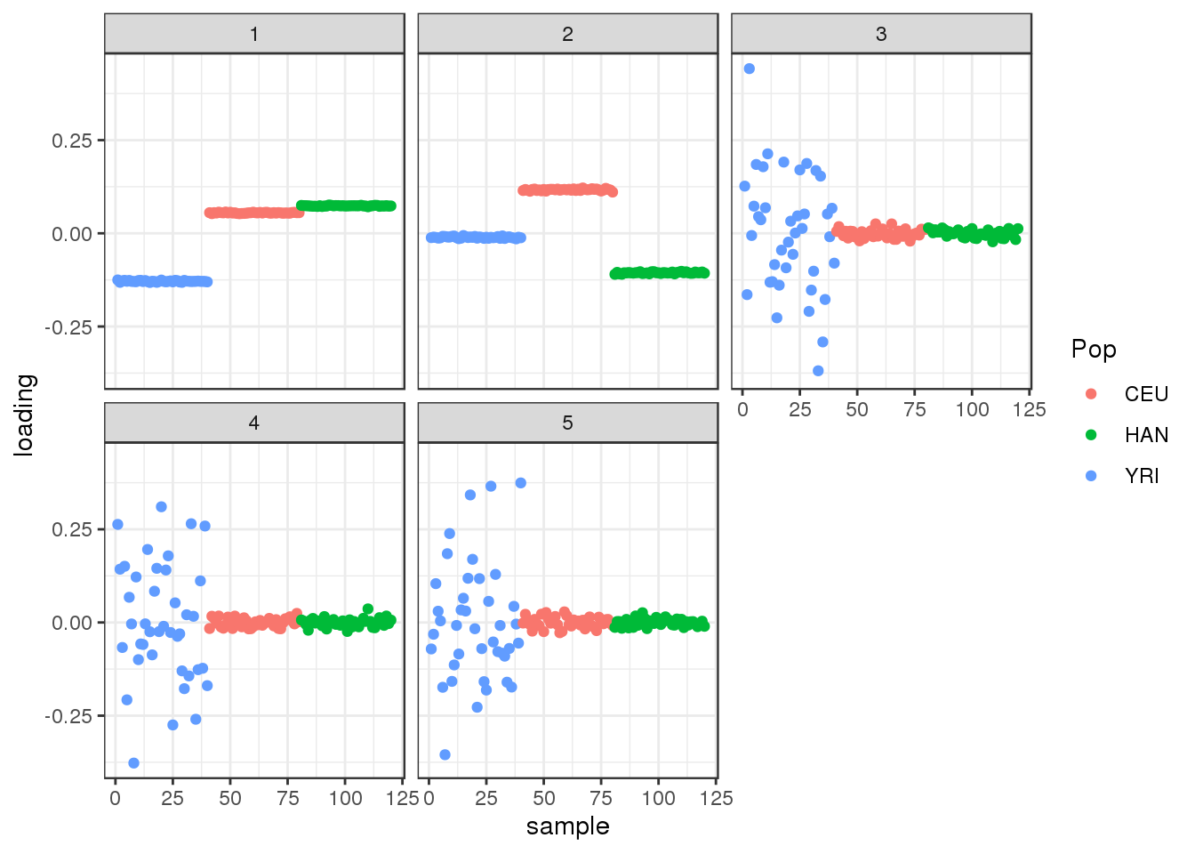
| Version | Author | Date |
|---|---|---|
| da3995d | Joseph Marcus | 2020-05-12 |
Plot the first two factors against each other:
qplot(L_hat[,1], L_hat[,2], color=labs) +
  xlab("PC1") +
  ylab("PC2") +
  theme_bw()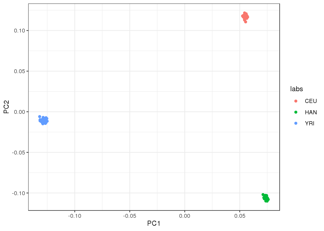
| Version | Author | Date |
|---|---|---|
| da3995d | Joseph Marcus | 2020-05-12 |
We certainly detect “clustered” population structure in the top PCs where PC1 represents Out of Africa and PC2 represents the next split between CEU and HAN.
ALStructure
Run ALStructure with \(K=3\):
admix_res <- alstructure::alstructure(t(Y), d_hat=3)
Qhat <- t(admix_res$Q_hat)
plot_loadings(Qhat, labs)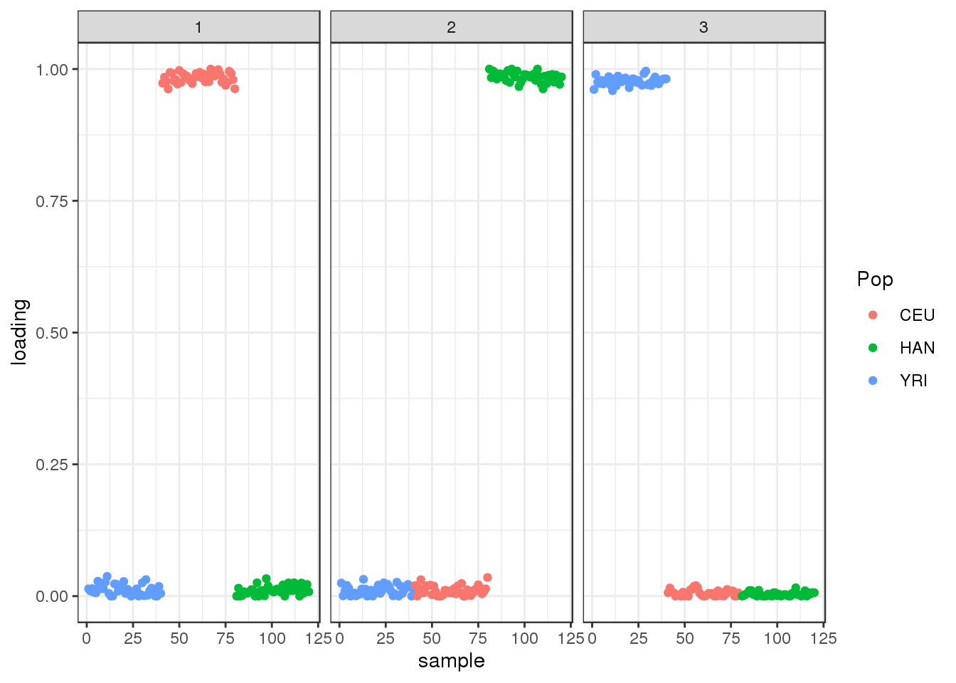
| Version | Author | Date |
|---|---|---|
| da3995d | Joseph Marcus | 2020-05-12 |
the PSD model assigns three distinct clusters.
flash [greedy]
Run the greedy algorithm:
fl <- flash(Y,
            greedy.Kmax=5,
            prior.family=c(prior.bimodal(), prior.normal()))
Adding factor 1 to flash object...
Adding factor 2 to flash object...
Adding factor 3 to flash object...
Adding factor 4 to flash object...
Adding factor 5 to flash object...
Factor doesn't significantly increase objective and won't be added.
Wrapping up...
Done.
Nullchecking 4 factors...
Done.plot_loadings(fl$flash.fit$EF[[1]], labs)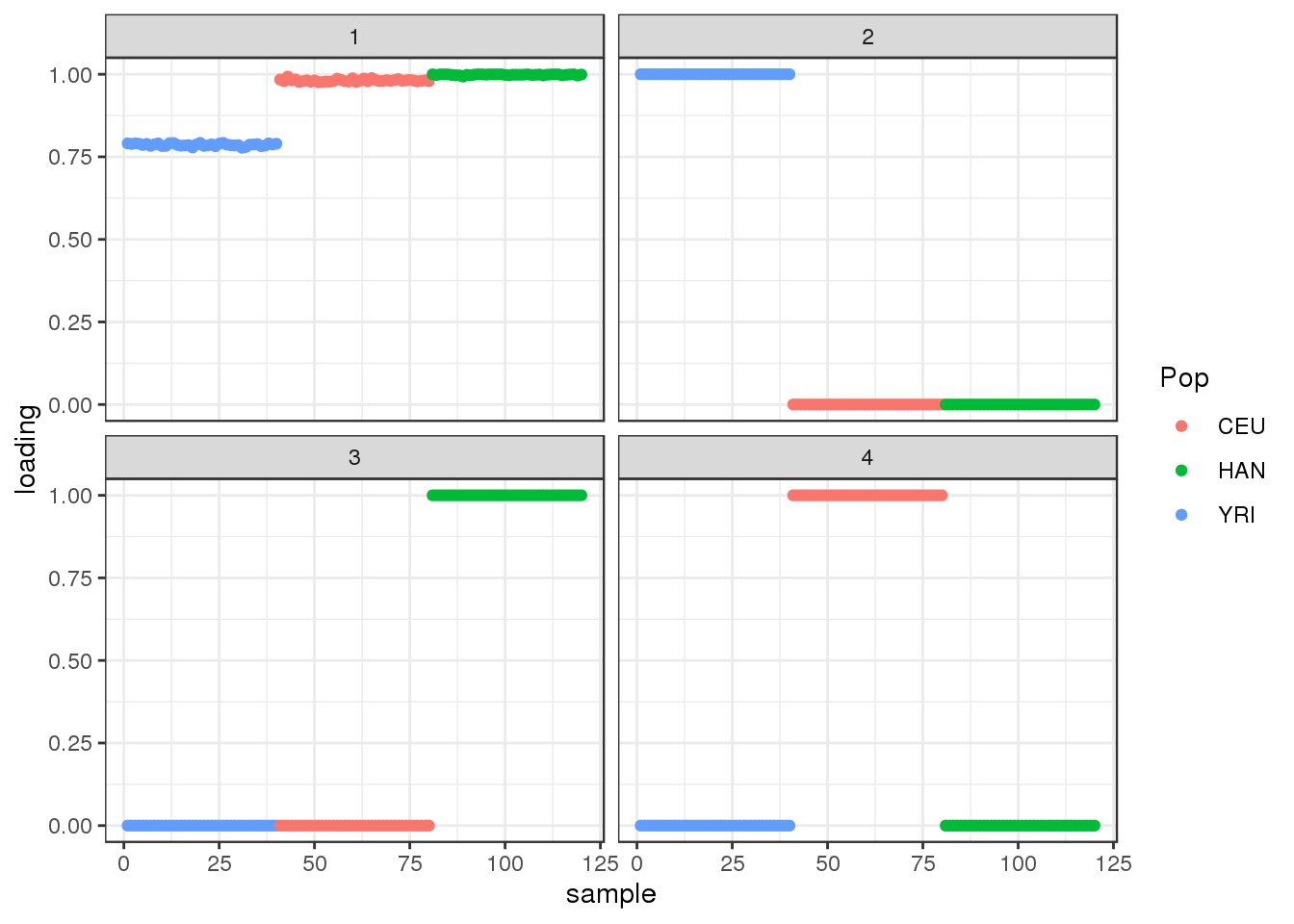
| Version | Author | Date |
|---|---|---|
| da3995d | Joseph Marcus | 2020-05-12 |
flash learns a shared factor between all the populations but where YRI has a lower loading then CEU and HAN and then it also learns population specific factors.
flash [backfit]
Run flash [backfit] initializing from the greedy solution:
flbf <- fl %>%
  flash.backfit() %>%
  flash.nullcheck(remove=TRUE)
Backfitting 4 factors (tolerance: 5.33e-02)...
Difference between iterations is within 1.0e+02...
Difference between iterations is within 1.0e+01...
Difference between iterations is within 1.0e+00...
Difference between iterations is within 1.0e-01...
Wrapping up...
Done.
Nullchecking 4 factors...
Wrapping up...
Done.plot_loadings(flbf$flash.fit$EF[[1]], labs)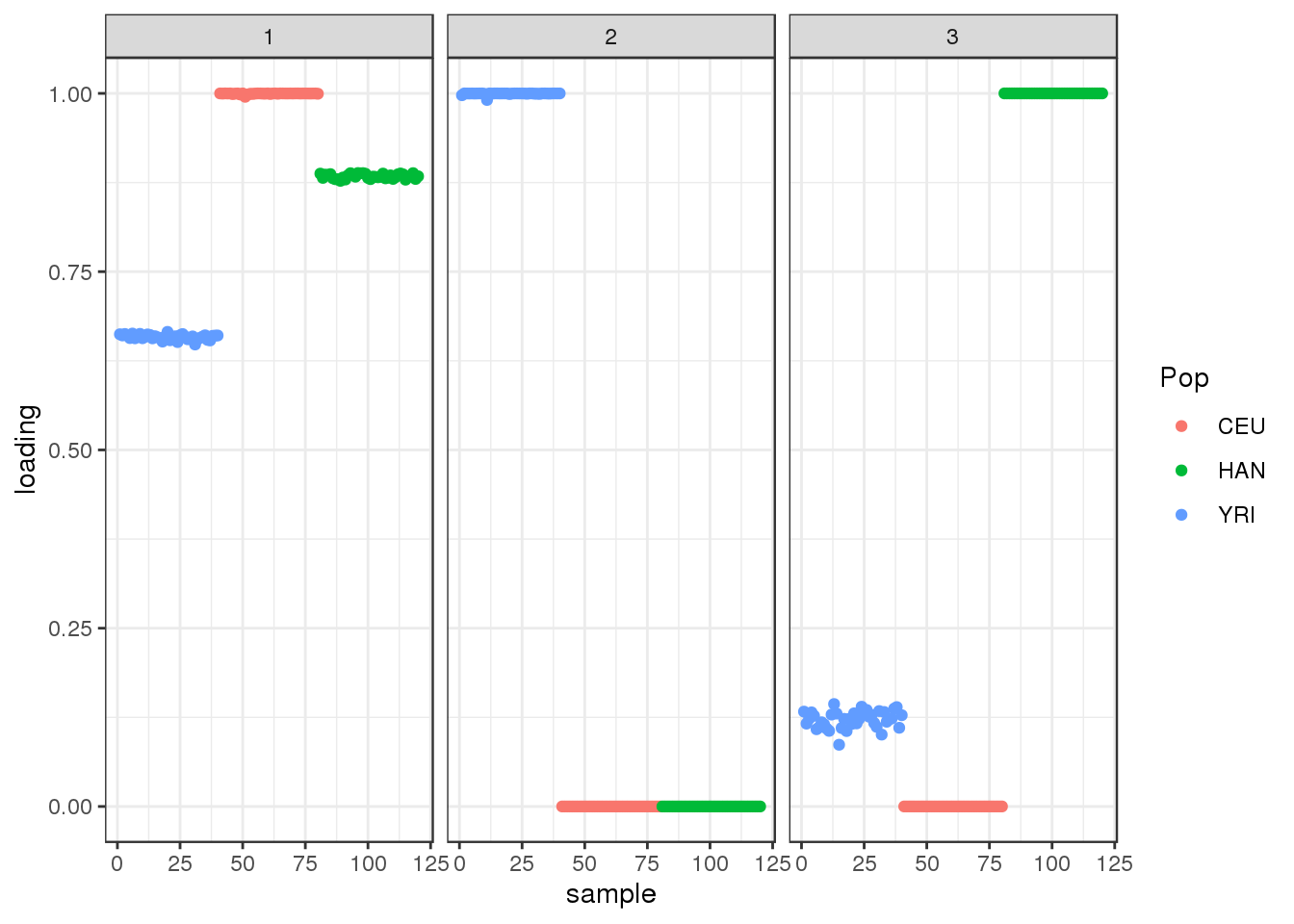
the backfitting algorithm represents the data with a sparser solution.
drift
Run drift initializing from the greedy solution:
init <- init_from_flash(fl)
dr <- drift(init, miniter=2, maxiter=500, tol=0.01, verbose=TRUE)
1 : -2865526.968
2 : -2864791.747
3 : -2864664.530
4 : -2864625.627
5 : -2864609.146
6 : -2864600.343
7 : -2864594.570
8 : -2864590.168
9 : -2864586.500
10 : -2864583.297
11 : -2864580.417
12 : -2864577.764
13 : -2864575.242
14 : -2864572.738
15 : -2864570.080
16 : -2864566.973
17 : -2864562.840
18 : -2864556.457
19 : -2864545.166
20 : -2864527.208
21 : -2864518.747
22 : -2864518.001
23 : -2864517.676
24 : -2864517.424
25 : -2864517.226
26 : -2864517.071
27 : -2864516.949
28 : -2864516.853
29 : -2864516.777
30 : -2864516.717
31 : -2864516.670
32 : -2864516.632
33 : -2864516.603
34 : -2864516.579
35 : -2864516.561
36 : -2864516.546
37 : -2864516.534
38 : -2864516.525 plot_loadings(dr$EL, labs)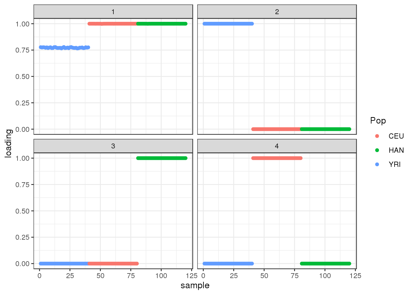
| Version | Author | Date |
|---|---|---|
| da3995d | Joseph Marcus | 2020-05-12 |
drift seems to maintain the greedy solution.
sessionInfo()R version 3.5.1 (2018-07-02)
Platform: x86_64-pc-linux-gnu (64-bit)
Running under: Scientific Linux 7.4 (Nitrogen)
Matrix products: default
BLAS/LAPACK: /software/openblas-0.2.19-el7-x86_64/lib/libopenblas_haswellp-r0.2.19.so
locale:
[1] LC_CTYPE=en_US.UTF-8 LC_NUMERIC=C
[3] LC_TIME=en_US.UTF-8 LC_COLLATE=en_US.UTF-8
[5] LC_MONETARY=en_US.UTF-8 LC_MESSAGES=en_US.UTF-8
[7] LC_PAPER=en_US.UTF-8 LC_NAME=C
[9] LC_ADDRESS=C LC_TELEPHONE=C
[11] LC_MEASUREMENT=en_US.UTF-8 LC_IDENTIFICATION=C
attached base packages:
[1] stats graphics grDevices utils datasets methods base
other attached packages:
[1] alstructure_0.1.0 forcats_0.5.0 stringr_1.4.0
[4] dplyr_0.8.5 purrr_0.3.4 readr_1.3.1
[7] tidyr_1.0.2 tibble_3.0.1 tidyverse_1.3.0
[10] reshape2_1.4.3 ggplot2_3.3.0 drift.alpha_0.0.9
[13] flashier_0.2.4 lfa_1.9.0
loaded via a namespace (and not attached):
[1] httr_1.4.1 jsonlite_1.6 modelr_0.1.6 assertthat_0.2.1
[5] mixsqp_0.3-17 cellranger_1.1.0 yaml_2.2.0 ebnm_0.1-24
[9] pillar_1.4.3 backports_1.1.6 lattice_0.20-38 glue_1.4.0
[13] digest_0.6.25 promises_1.0.1 rvest_0.3.5 colorspace_1.4-1
[17] htmltools_0.3.6 httpuv_1.4.5 Matrix_1.2-15 plyr_1.8.4
[21] pkgconfig_2.0.3 invgamma_1.1 broom_0.5.6 haven_2.2.0
[25] corpcor_1.6.9 scales_1.1.0 whisker_0.3-2 later_0.7.5
[29] git2r_0.26.1 farver_2.0.3 generics_0.0.2 ellipsis_0.3.0
[33] withr_2.2.0 ashr_2.2-50 cli_2.0.2 magrittr_1.5
[37] crayon_1.3.4 readxl_1.3.1 evaluate_0.14 fs_1.3.1
[41] fansi_0.4.1 nlme_3.1-137 xml2_1.3.2 truncnorm_1.0-8
[45] tools_3.5.1 hms_0.5.3 lifecycle_0.2.0 munsell_0.5.0
[49] reprex_0.3.0 irlba_2.3.3 compiler_3.5.1 rlang_0.4.5
[53] grid_3.5.1 rstudioapi_0.11 labeling_0.3 rmarkdown_1.10
[57] gtable_0.3.0 DBI_1.0.0 R6_2.4.1 lubridate_1.7.4
[61] knitr_1.20 workflowr_1.6.1 rprojroot_1.3-2 stringi_1.4.6
[65] parallel_3.5.1 SQUAREM_2020.2 Rcpp_1.0.4.6 vctrs_0.2.4
[69] dbplyr_1.4.3 tidyselect_1.0.0