AmericanAdmixture_4B11_fix
Joseph Marcus
2020-05-18
Last updated: 2020-05-21
Checks: 7 0
Knit directory: drift-workflow/analysis/
This reproducible R Markdown analysis was created with workflowr (version 1.6.1). The Checks tab describes the reproducibility checks that were applied when the results were created. The Past versions tab lists the development history.
Great! Since the R Markdown file has been committed to the Git repository, you know the exact version of the code that produced these results.
Great job! The global environment was empty. Objects defined in the global environment can affect the analysis in your R Markdown file in unknown ways. For reproduciblity it’s best to always run the code in an empty environment.
The command set.seed(20190211) was run prior to running the code in the R Markdown file. Setting a seed ensures that any results that rely on randomness, e.g. subsampling or permutations, are reproducible.
Great job! Recording the operating system, R version, and package versions is critical for reproducibility.
Nice! There were no cached chunks for this analysis, so you can be confident that you successfully produced the results during this run.
Great job! Using relative paths to the files within your workflowr project makes it easier to run your code on other machines.
Great! You are using Git for version control. Tracking code development and connecting the code version to the results is critical for reproducibility.
The results in this page were generated with repository version da22c75. See the Past versions tab to see a history of the changes made to the R Markdown and HTML files.
Note that you need to be careful to ensure that all relevant files for the analysis have been committed to Git prior to generating the results (you can use wflow_publish or wflow_git_commit). workflowr only checks the R Markdown file, but you know if there are other scripts or data files that it depends on. Below is the status of the Git repository when the results were generated:
Ignored files:
    Ignored:    .snakemake/
    Ignored:    data/datasets/
    Ignored:    data/raw/
    Ignored:    data/simulations/
    Ignored:    notebooks/.ipynb_checkpoints/
    Ignored:    output/
    Ignored:    sandbox/.ipynb_checkpoints/

Unstaged changes:
    Modified:   analysis/OutOfAfrica_3G09_fix.Rmd
Note that any generated files, e.g. HTML, png, CSS, etc., are not included in this status report because it is ok for generated content to have uncommitted changes.
These are the previous versions of the repository in which changes were made to the R Markdown (analysis/AmericanAdmixture_4B11_fix.Rmd) and HTML (docs/AmericanAdmixture_4B11_fix.html) files. If you’ve configured a remote Git repository (see ?wflow_git_remote), click on the hyperlinks in the table below to view the files as they were in that past version.
| File | Version | Author | Date | Message |
|---|---|---|---|---|
| Rmd | da22c75 | Joseph Marcus | 2020-05-21 | wflow_publish(“AmericanAdmixture_4B11_fix.Rmd”) |
| html | 87a17c5 | Joseph Marcus | 2020-05-21 | Build site. |
| Rmd | 2e57d3d | Joseph Marcus | 2020-05-21 | wflow_publish(“AmericanAdmixture_4B11_fix.Rmd”) |
Here I visualize population structure with simulated data from the AmericanAdmixture_4B11 scenario. See Browning et al. 2018 for details.
Below, I show a number of EBMF solutions and in each of them I don’t display the first shared factor which is prefixed to the one-vector and scale the loadings by the prior variance. I only describe the loadings that remain after the shared factor.
Imports
Import the required libraries and scripts:
suppressMessages({
  library(lfa)
  library(flashier)
  library(drift.alpha)
  library(ggplot2)
  library(RColorBrewer)
  library(reshape2)
  library(tidyverse)
  library(alstructure)
  source("../code/structure_plot.R")
})
Data
data_path <- "../output/simulations/AmericanAdmixture_4B11/rep2.txt"
G <- t(as.matrix(read.table(data_path, sep=" ")))
colnames(G) <- NULL
rownames(G) <- NULL
n <- nrow(G)
daf <- colSums(G) / (2 * n)
colors <- brewer.pal(8, "Set2")

# filter out too rare and too common SNPs
Y <- G[,((daf>=.05) & (daf <=.95))]
p <- ncol(Y)
print(n)
[1] 160print(p)[1] 25026# sub-population labels from stdpop
labs <- rep(c("AFR", "EUR", "ASIA", "ADMIX"), each=40)we end up with 160 individuals and ~25000 SNPs. View fitted the sample covariance matrix:
plot_cov((1.0 / p) * Y %*% t(Y), as.is=T)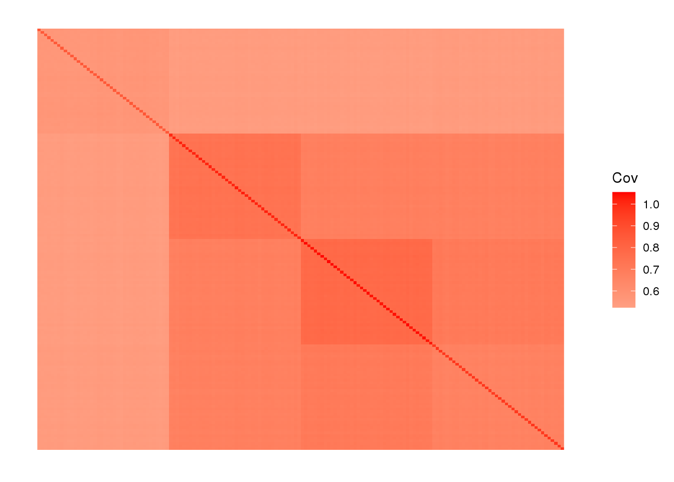
| Version | Author | Date |
|---|---|---|
| 87a17c5 | Joseph Marcus | 2020-05-21 |
flash [greedy]
Run the greedy algorithm:
ones <- matrix(1, nrow = n, ncol = 1)
ls.soln <- t(solve(crossprod(ones), crossprod(ones, Y)))
fl <- flash.init(Y) %>%
  flash.init.factors(EF = list(ones, ls.soln),
                     prior.family=c(prior.bimodal(), prior.normal())) %>%
  flash.fix.loadings(kset = 1, mode = 1L) %>%
  flash.backfit() %>%
  flash.add.greedy(Kmax=8, prior.family=c(prior.bimodal(), prior.normal()))
Backfitting 1 factors (tolerance: 5.97e-02)...
Difference between iterations is within 1.0e-01...
Wrapping up...
Done.
Adding factor 2 to flash object...
Adding factor 3 to flash object...
Adding factor 4 to flash object...
Adding factor 5 to flash object...
Factor doesn't significantly increase objective and won't be added.
Wrapping up...
Done.sd <- unlist(lapply(fl$fitted.g[[2]], '[[', 3))
L <- fl$flash.fit$EF[[1]]
LDsqrt <- L %*% diag(sd)
K <- ncol(LDsqrt)
plot_loadings(LDsqrt[,2:K], labs) + scale_color_brewer(palette="Set2")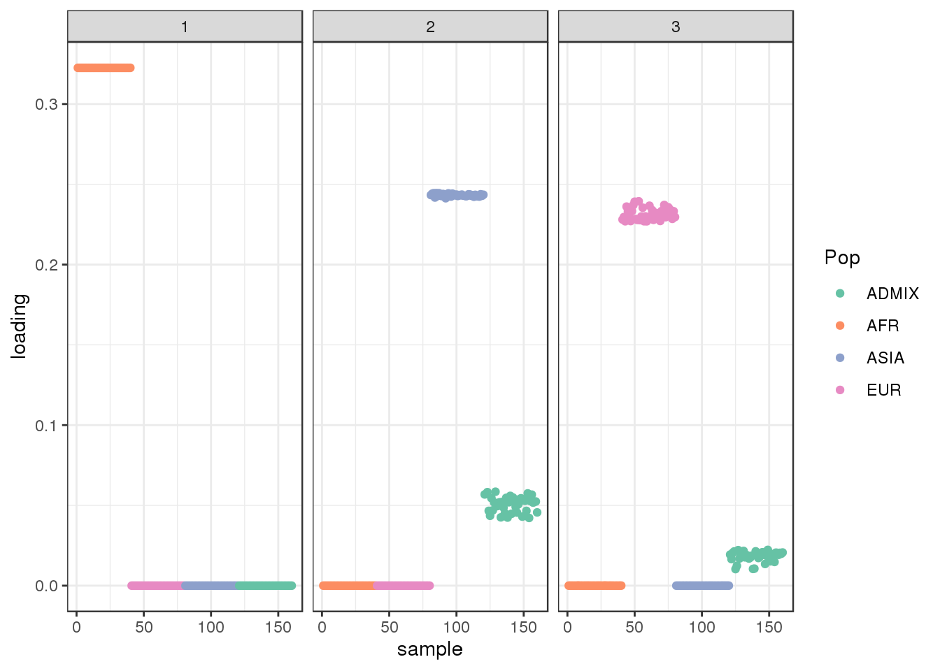
| Version | Author | Date |
|---|---|---|
| 87a17c5 | Joseph Marcus | 2020-05-21 |
view structure plot:
create_structure_plot(L=LDsqrt[,2:K], labels=labs, colors=colors)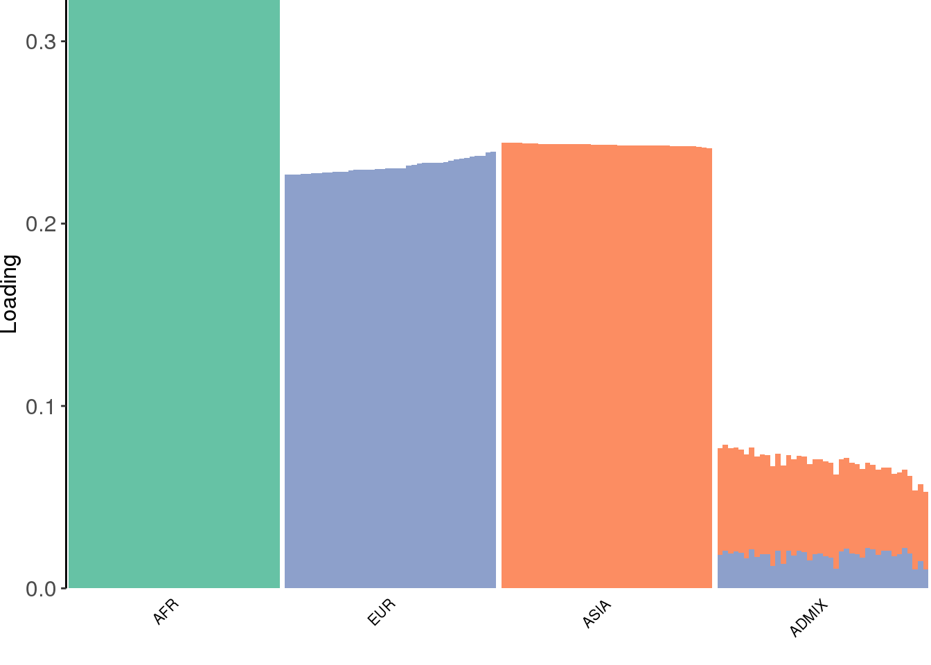
| Version | Author | Date |
|---|---|---|
| 87a17c5 | Joseph Marcus | 2020-05-21 |
view fitted covariance matrix:
plot_cov(LDsqrt %*% t(LDsqrt), as.is=T)
| Version | Author | Date |
|---|---|---|
| 87a17c5 | Joseph Marcus | 2020-05-21 |
the greedy algorithm picks up a bit of a signal of admixture but misses out on the African contribution.
flash [backfit]
Run flash [backfit] initializing from the greedy solution:
flbf <- fl %>%
  flash.backfit() %>%
  flash.nullcheck(remove=TRUE)
Backfitting 4 factors (tolerance: 5.97e-02)...
Difference between iterations is within 1.0e+03...
Difference between iterations is within 1.0e+02...
Difference between iterations is within 1.0e+01...
Difference between iterations is within 1.0e+00...
Difference between iterations is within 1.0e-01...
Difference between iterations is within 1.0e-02...
Wrapping up...
Done.
Nullchecking 4 factors...
Done.sd <- unlist(lapply(flbf$fitted.g[[2]], '[[', 3))
L <- flbf$flash.fit$EF[[1]]
LDsqrt <- L %*% diag(sd)
K <- ncol(LDsqrt)
plot_loadings(LDsqrt[,2:K], labs) + scale_color_brewer(palette="Set2")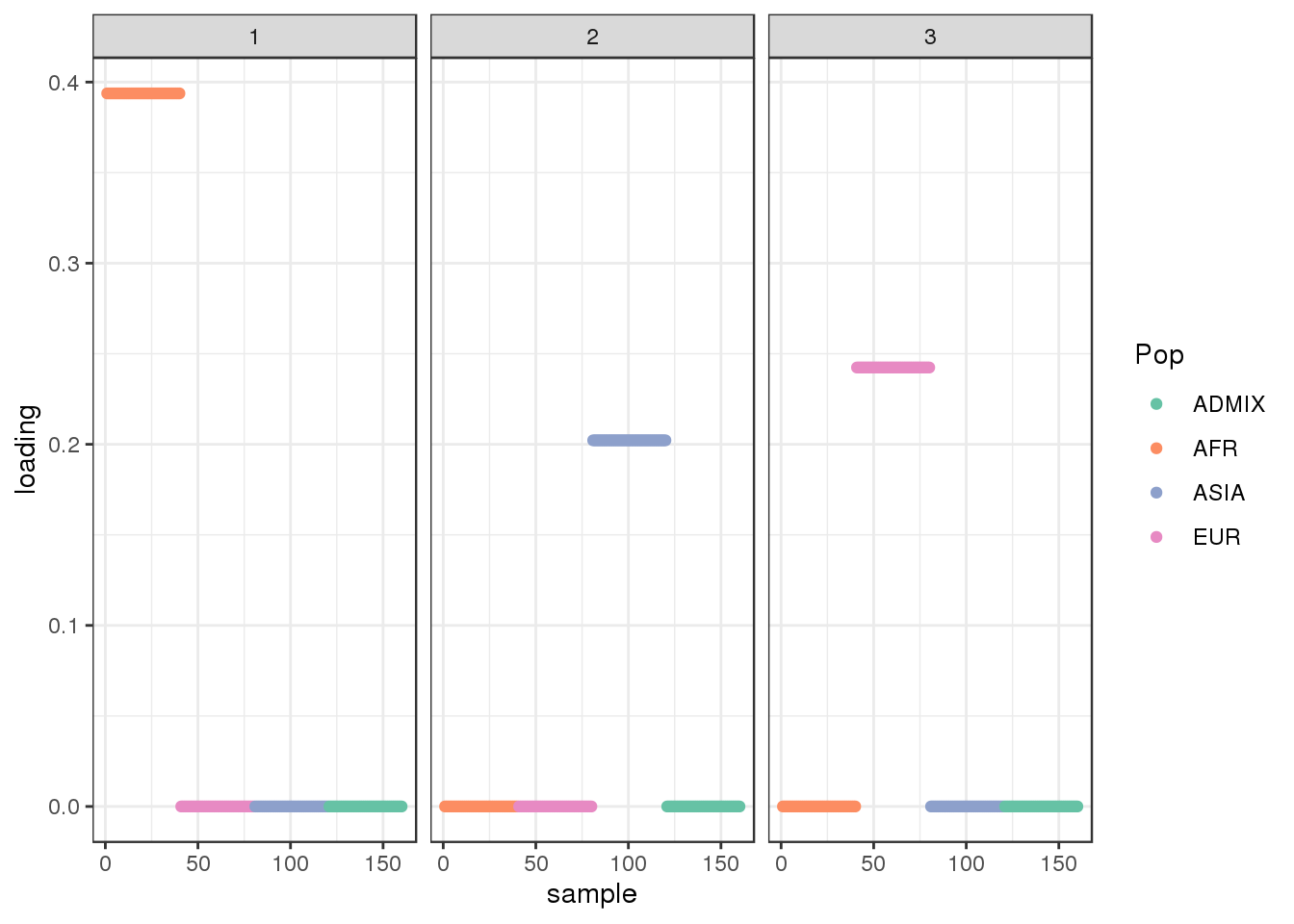
| Version | Author | Date |
|---|---|---|
| 87a17c5 | Joseph Marcus | 2020-05-21 |
view structure plot:
create_structure_plot(L=LDsqrt[,2:K], labels=labs, colors=colors)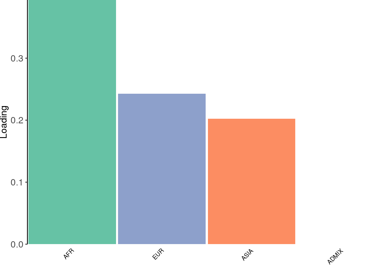
| Version | Author | Date |
|---|---|---|
| 87a17c5 | Joseph Marcus | 2020-05-21 |
view fitted covariance matrix:
plot_cov(LDsqrt %*% t(LDsqrt), as.is=T)
| Version | Author | Date |
|---|---|---|
| 87a17c5 | Joseph Marcus | 2020-05-21 |
The backfitting algorithm misses out on the signal of admixture and finds only 3 population specific factors after the shared factor.
drift
Run drift initializing from the greedy solution:
init <- init_from_data(Y, Kmax=6)
dr <- drift(init, miniter=2,
            maxiter=1000,
            tol=0.01,
            verbose=FALSE)

sd <- sqrt(dr$prior_s2)
L <- dr$EL
LDsqrt <- L %*% diag(sd)
K <- ncol(LDsqrt)
plot_loadings(LDsqrt[,2:K], labs) + scale_color_brewer(palette="Set2")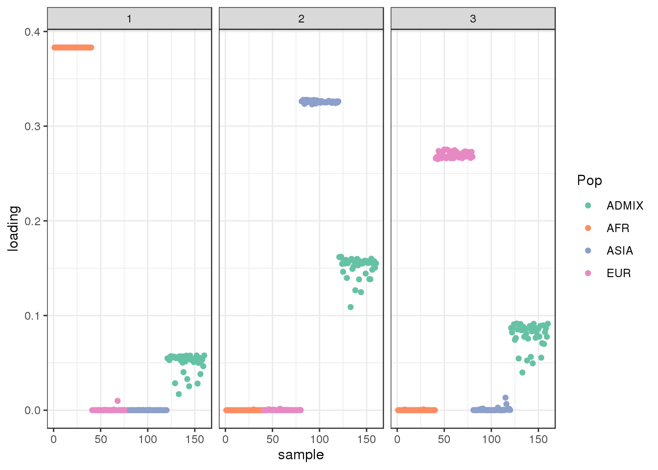
| Version | Author | Date |
|---|---|---|
| 87a17c5 | Joseph Marcus | 2020-05-21 |
view structure plot:
create_structure_plot(L=LDsqrt[,2:K], labels=labs, colors=colors)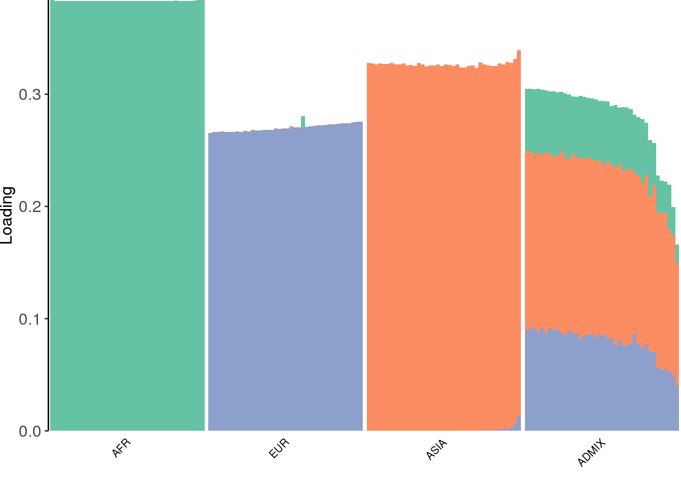
| Version | Author | Date |
|---|---|---|
| 87a17c5 | Joseph Marcus | 2020-05-21 |
view fitted covariance matrix:
plot_cov(LDsqrt %*% t(LDsqrt), as.is=T)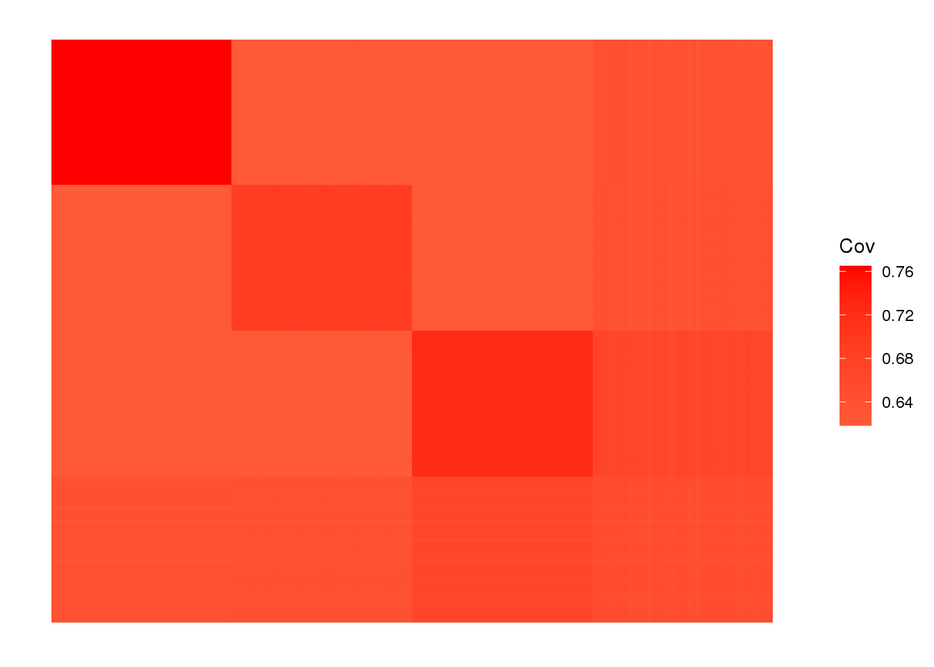
| Version | Author | Date |
|---|---|---|
| 87a17c5 | Joseph Marcus | 2020-05-21 |
drift much better represents the admixture signal but misses the EUR/ASIA two population factor.
sessionInfo()R version 3.5.1 (2018-07-02)
Platform: x86_64-pc-linux-gnu (64-bit)
Running under: Scientific Linux 7.4 (Nitrogen)
Matrix products: default
BLAS/LAPACK: /software/openblas-0.2.19-el7-x86_64/lib/libopenblas_haswellp-r0.2.19.so
locale:
[1] LC_CTYPE=en_US.UTF-8 LC_NUMERIC=C
[3] LC_TIME=en_US.UTF-8 LC_COLLATE=en_US.UTF-8
[5] LC_MONETARY=en_US.UTF-8 LC_MESSAGES=en_US.UTF-8
[7] LC_PAPER=en_US.UTF-8 LC_NAME=C
[9] LC_ADDRESS=C LC_TELEPHONE=C
[11] LC_MEASUREMENT=en_US.UTF-8 LC_IDENTIFICATION=C
attached base packages:
[1] stats graphics grDevices utils datasets methods base
other attached packages:
[1] alstructure_0.1.0 forcats_0.5.0 stringr_1.4.0
[4] dplyr_0.8.5 purrr_0.3.4 readr_1.3.1
[7] tidyr_1.0.2 tibble_3.0.1 tidyverse_1.3.0
[10] reshape2_1.4.3 RColorBrewer_1.1-2 ggplot2_3.3.0
[13] drift.alpha_0.0.9 flashier_0.2.4 lfa_1.9.0
loaded via a namespace (and not attached):
[1] httr_1.4.1 jsonlite_1.6 modelr_0.1.6 assertthat_0.2.1
[5] mixsqp_0.3-43 cellranger_1.1.0 yaml_2.2.0 ebnm_0.1-24
[9] pillar_1.4.3 backports_1.1.6 lattice_0.20-38 glue_1.4.0
[13] digest_0.6.25 promises_1.0.1 rvest_0.3.5 colorspace_1.4-1
[17] htmltools_0.3.6 httpuv_1.4.5 Matrix_1.2-15 plyr_1.8.4
[21] pkgconfig_2.0.3 invgamma_1.1 broom_0.5.6 haven_2.2.0
[25] corpcor_1.6.9 scales_1.1.0 whisker_0.3-2 later_0.7.5
[29] git2r_0.26.1 farver_2.0.3 generics_0.0.2 ellipsis_0.3.0
[33] withr_2.2.0 ashr_2.2-50 cli_2.0.2 magrittr_1.5
[37] crayon_1.3.4 readxl_1.3.1 evaluate_0.14 fansi_0.4.1
[41] fs_1.3.1 nlme_3.1-137 xml2_1.3.2 truncnorm_1.0-8
[45] tools_3.5.1 hms_0.5.3 lifecycle_0.2.0 munsell_0.5.0
[49] reprex_0.3.0 irlba_2.3.3 compiler_3.5.1 rlang_0.4.5
[53] grid_3.5.1 rstudioapi_0.11 labeling_0.3 rmarkdown_1.10
[57] gtable_0.3.0 DBI_1.0.0 R6_2.4.1 lubridate_1.7.4
[61] knitr_1.20 workflowr_1.6.1 rprojroot_1.3-2 stringi_1.4.6
[65] parallel_3.5.1 SQUAREM_2020.2 Rcpp_1.0.4.6 vctrs_0.2.4
[69] dbplyr_1.4.3 tidyselect_1.0.0