Human Origins Array West Eurasia Results

Last updated: 2019-02-15

workflowr checks: (Click a bullet for more information)

✔ R Markdown file: up-to-date

Great! Since the R Markdown file has been committed to the Git repository, you know the exact version of the code that produced these results.
✔ Environment: empty

Great job! The global environment was empty. Objects defined in the global environment can affect the analysis in your R Markdown file in unknown ways. For reproduciblity it’s best to always run the code in an empty environment.
✔ Seed: set.seed(20190211)

The command set.seed(20190211) was run prior to running the code in the R Markdown file. Setting a seed ensures that any results that rely on randomness, e.g. subsampling or permutations, are reproducible.
✔ Session information: recorded

Great job! Recording the operating system, R version, and package versions is critical for reproducibility.
✔ Repository version: 7a2b6c7
Great! You are using Git for version control. Tracking code development and connecting the code version to the results is critical for reproducibility. The version displayed above was the version of the Git repository at the time these results were generated.

Note that you need to be careful to ensure that all relevant files for the analysis have been committed to Git prior to generating the results (you can use wflow_publish or wflow_git_commit). workflowr only checks the R Markdown file, but you know if there are other scripts or data files that it depends on. Below is the status of the Git repository when the results were generated:
```
Ignored files:
    Ignored:    .Rhistory
    Ignored:    Makefile
    Ignored:    analysis/flash_cache/
    Ignored:    data/.DS_Store
    Ignored:    data/raw/
    Ignored:    output/admixture/
    Ignored:    output/flash_backfit/
    Ignored:    output/flash_greedy/
    Ignored:    output/softImpute/

Unstaged changes:
    Modified:   analysis/hoa_global.Rmd
```
Note that any generated files, e.g. HTML, png, CSS, etc., are not included in this status report because it is ok for generated content to have uncommitted changes.

Expand here to see past versions:

File	Version	Author	Date	Message
Rmd	7a2b6c7	jhmarcus	2019-02-15	added backfit
html	7a2b6c7	jhmarcus	2019-02-15	added backfit
Rmd	f5ef1af	jhmarcus	2019-02-15	added workflows for human origins datasets
html	f5ef1af	jhmarcus	2019-02-15	added workflows for human origins datasets

Imports

Lets import some needed packages

library(ggplot2)
library(tidyr)
library(dplyr)
library(RColorBrewer)
source("../code/viz.R")
getPalette = colorRampPalette(brewer.pal(12, "Set3"))

Human Origins West Eurasia (LD Pruned)

This is a subset of the Human Origins Array dataset with 770 sampled from across West Eurasia. I filtered out rare variants with global minor allele frequency less than 5%, and remove any variants with a missingness level greater than 1%. I then LD pruned the SNPs using standard parameters in plink, resulting in 139640 SNPs.

Greedy

Lets first read the greedy flashier fit

flash_fit = readRDS("../output/flash_greedy/hoa_weurasia_ld/HumanOriginsPublic2068_weurasia_maf_geno_ldprune.rds")
K = ncol(flash_fit$loadings$normalized.loadings[[1]]) 
n = nrow(flash_fit$loadings$normalized.loadings[[1]])
p = nrow(flash_fit$loadings$normalized.loadings[[2]])
print(K)

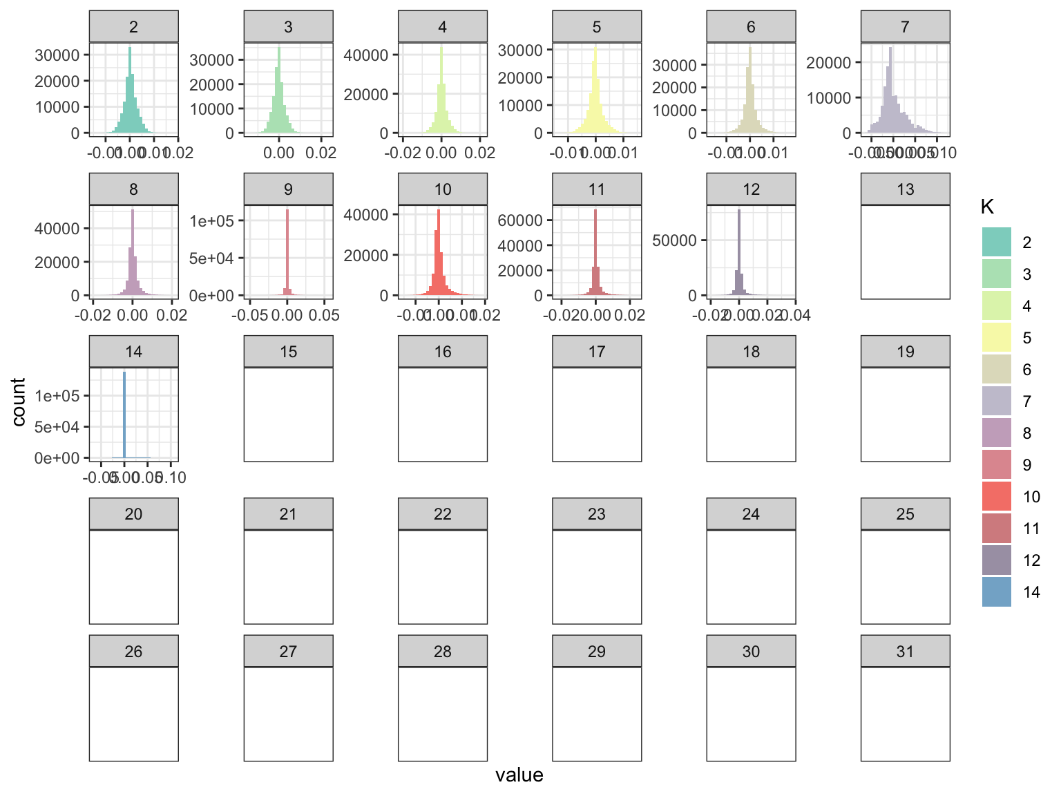
[1] 31

print(n)

[1] 770

print(p)

[1] 139640

Lets now plot the distribution of factors for each drift event

# read factors
delta_df = as.data.frame(flash_fit$loadings$normalized.loadings[[2]])
colnames(delta_df)[1:K] = 1:K 

# gather the data.frame for plotting
delta_gath_df = delta_df %>% 
                gather(K, value) %>%
                filter(K!=1)

# plot the factors
K_ = K
p_fct = ggplot(delta_gath_df, aes(x=value, fill=factor(K, 2:K_))) + 
        scale_fill_manual(values = getPalette(K_)) +
        geom_histogram() + 
        facet_wrap(~factor(K, levels=2:K_), scales = "free") + 
        labs(fill="K") + 
        scale_x_continuous(breaks = scales::pretty_breaks(n = 3)) +
        scale_y_continuous(breaks = scales::pretty_breaks(n = 3)) + 
        theme_bw()
p_fct

Expand here to see past versions of flash-greedy-ld-viz-factors-1.png:

Version	Author	Date
f5ef1af	jhmarcus	2019-02-15

This seems that greedyflashier found no contributions of factors after the 14th although it seems a little bit buggy b/c the 13th factor is all NA but the 14th factor has some non-zeros but it does indeed seem very sparse? Lets now take a look at the loadings:

# read the meta data
meta_df = read.table("../data/meta/HumanOriginsPublic2068_weurasia_maf_geno_ldprune.meta", sep=" ", header=T)

# setup loadings data.frame
l_df = as.data.frame(flash_fit$loadings$normalized.loadings[[1]])
l_df$iid = meta_df$iid # individual ids
l_df$clst = meta_df$clst # population labels

# join with the meta data
l_df = l_df %>% inner_join(meta_df, on="clst")
l_df = l_df %>% arrange(region, clst) # sort by region then by population
l_df$iid = factor(l_df$iid, levels = l_df$iid) # make sure the ids are sorted
colnames(l_df)[1:K] = 1:K

l_df = l_df %>% select_if(~sum(!is.na(.)) > 0)

# gather the data.frame for plotting
l_gath_df = l_df %>% 
            gather(K, value, -iid, -clst, -region, -country, -lat, -lon, -clst2) %>% 
            filter(K!=1) 

#### viz #####
pops = unique(l_df$clst)

# West Eurasia
west_eurasia_pops = get_pops(meta_df, "WestEurasia")
p_west_eurasia = positive_structure_plot(l_gath_df, west_eurasia_pops, K, label_size=5)
p_west_eurasia

Expand here to see past versions of flash-greedy-ld-viz-loadings-1.png:

Version	Author	Date
f5ef1af	jhmarcus	2019-02-15

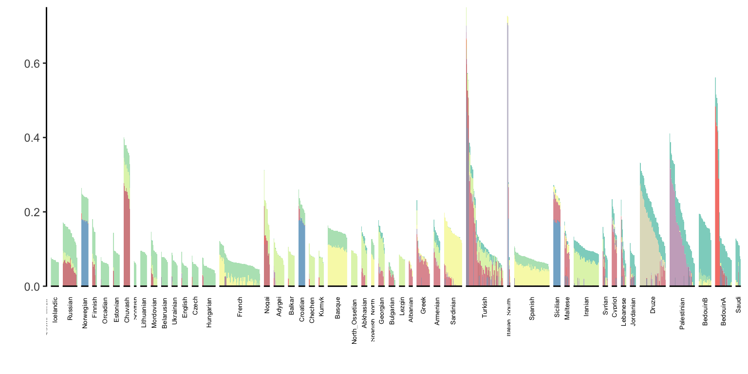
It does seem cool that many groups can be made up of a sparse set of colors but it looks like many groups can be quite noisy as well.

Backfitting

flash_fit = readRDS("../output/flash_backfit/hoa_weurasia_ld/HumanOriginsPublic2068_weurasia_maf_geno_ldprune.rds")
K = ncol(flash_fit$loadings$normalized.loadings[[1]]) 
n = nrow(flash_fit$loadings$normalized.loadings[[1]])
p = nrow(flash_fit$loadings$normalized.loadings[[2]])
print(K)

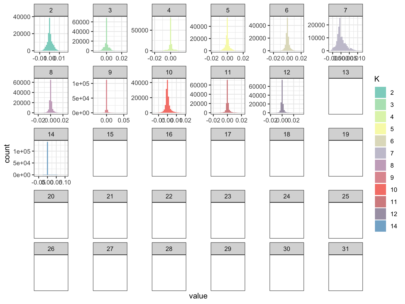
[1] 31

print(n)

[1] 770

print(p)

[1] 139640

Lets now plot the distribution of factors for each drift event

# read factors
delta_df = as.data.frame(flash_fit$loadings$normalized.loadings[[2]])
colnames(delta_df)[1:K] = 1:K 

# gather the data.frame for plotting
delta_gath_df = delta_df %>% 
                gather(K, value) %>%
                filter(K!=1)

# plot the factors
K_ = K
p_fct = ggplot(delta_gath_df, aes(x=value, fill=factor(K, 2:K_))) + 
        scale_fill_manual(values = getPalette(K_)) +
        geom_histogram() + 
        facet_wrap(~factor(K, levels=2:K_), scales = "free") + 
        labs(fill="K") + 
        scale_x_continuous(breaks = scales::pretty_breaks(n = 3)) +
        scale_y_continuous(breaks = scales::pretty_breaks(n = 3)) + 
        theme_bw()
p_fct

Expand here to see past versions of flash-backfit-ld-viz-factors-1.png:

Version	Author	Date
7a2b6c7	jhmarcus	2019-02-15

The factors look a bit sparser? Lets now look at the loadings:

# read the meta data
meta_df = read.table("../data/meta/HumanOriginsPublic2068_weurasia_maf_geno_ldprune.meta", sep=" ", header=T)

# setup loadings data.frame
l_df = as.data.frame(flash_fit$loadings$normalized.loadings[[1]])
l_df$iid = meta_df$iid # individual ids
l_df$clst = meta_df$clst # population labels

# join with the meta data
l_df = l_df %>% inner_join(meta_df, on="clst")
l_df = l_df %>% arrange(region, clst) # sort by region then by population
l_df$iid = factor(l_df$iid, levels = l_df$iid) # make sure the ids are sorted
colnames(l_df)[1:K] = 1:K

l_df = l_df %>% select_if(~sum(!is.na(.)) > 0)

# gather the data.frame for plotting
l_gath_df = l_df %>% 
            gather(K, value, -iid, -clst, -region, -country, -lat, -lon, -clst2) %>% 
            filter(K!=1) 

#### viz #####
pops = unique(l_df$clst)

# West Eurasia
west_eurasia_pops = get_pops(meta_df, "WestEurasia")
p_west_eurasia = positive_structure_plot(l_gath_df, west_eurasia_pops, K, label_size=5)
p_west_eurasia

Expand here to see past versions of flash-backfit-ld-viz-loadings-1.png:

Version	Author	Date
7a2b6c7	jhmarcus	2019-02-15

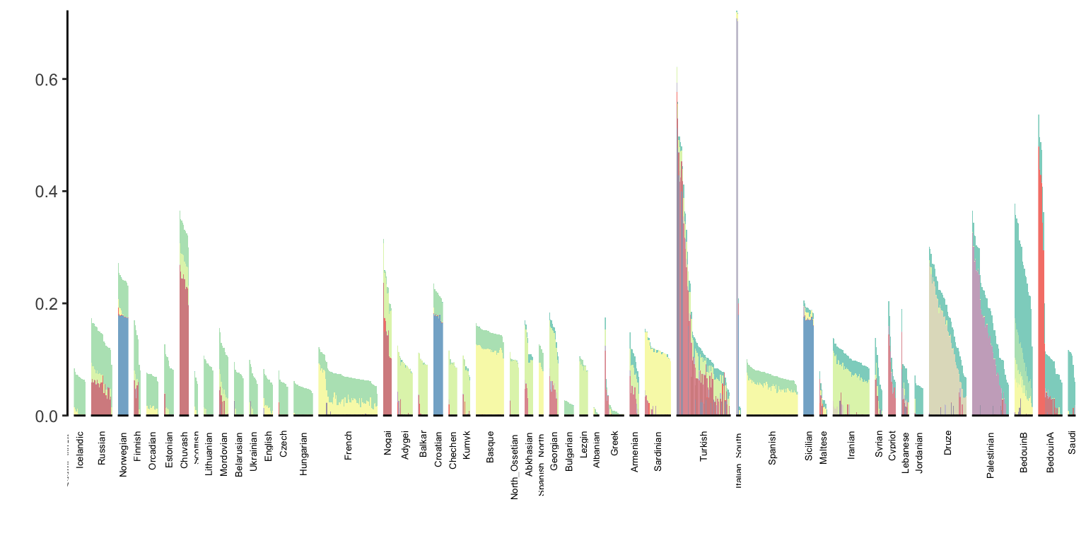
At first glance it doesn’t seem the backfitting changed much of the result.

Session information

sessionInfo()

R version 3.5.1 (2018-07-02)
Platform: x86_64-apple-darwin13.4.0 (64-bit)
Running under: macOS  10.14.2

Matrix products: default
BLAS/LAPACK: /Users/jhmarcus/miniconda3/lib/R/lib/libRblas.dylib

locale:
[1] en_US.UTF-8/en_US.UTF-8/en_US.UTF-8/C/en_US.UTF-8/en_US.UTF-8

attached base packages:
[1] stats     graphics  grDevices utils     datasets  methods   base     

other attached packages:
[1] bindrcpp_0.2.2     RColorBrewer_1.1-2 dplyr_0.7.6       
[4] tidyr_0.8.1        ggplot2_3.0.0     

loaded via a namespace (and not attached):
 [1] Rcpp_1.0.0        compiler_3.5.1    pillar_1.3.0     
 [4] git2r_0.23.0      plyr_1.8.4        workflowr_1.1.1  
 [7] bindr_0.1.1       R.methodsS3_1.7.1 R.utils_2.7.0    
[10] tools_3.5.1       digest_0.6.18     evaluate_0.12    
[13] tibble_1.4.2      gtable_0.2.0      pkgconfig_2.0.1  
[16] rlang_0.3.1       yaml_2.2.0        xfun_0.4         
[19] flashier_0.1.0    withr_2.1.2       stringr_1.3.1    
[22] knitr_1.21        rprojroot_1.3-2   grid_3.5.1       
[25] tidyselect_0.2.4  glue_1.3.0        R6_2.3.0         
[28] rmarkdown_1.11    reshape2_1.4.3    purrr_0.2.5      
[31] magrittr_1.5      whisker_0.3-2     backports_1.1.2  
[34] scales_0.5.0      htmltools_0.3.6   assertthat_0.2.0 
[37] colorspace_1.3-2  labeling_0.3      stringi_1.2.4    
[40] lazyeval_0.2.1    munsell_0.5.0     crayon_1.3.4     
[43] R.oo_1.22.0

This reproducible R Markdown analysis was created with workflowr 1.1.1