Mixed effects models
Last updated: 2021-06-15
Checks: 7 0
Knit directory: RainDrop_biodiversity/
This reproducible R Markdown analysis was created with workflowr (version 1.6.2). The Checks tab describes the reproducibility checks that were applied when the results were created. The Past versions tab lists the development history.
Great! Since the R Markdown file has been committed to the Git repository, you know the exact version of the code that produced these results.
Great job! The global environment was empty. Objects defined in the global environment can affect the analysis in your R Markdown file in unknown ways. For reproduciblity it’s best to always run the code in an empty environment.
The command set.seed(20210406) was run prior to running the code in the R Markdown file. Setting a seed ensures that any results that rely on randomness, e.g. subsampling or permutations, are reproducible.
Great job! Recording the operating system, R version, and package versions is critical for reproducibility.
Nice! There were no cached chunks for this analysis, so you can be confident that you successfully produced the results during this run.
Great job! Using relative paths to the files within your workflowr project makes it easier to run your code on other machines.
Great! You are using Git for version control. Tracking code development and connecting the code version to the results is critical for reproducibility.
The results in this page were generated with repository version cbc95ff. See the Past versions tab to see a history of the changes made to the R Markdown and HTML files.
Note that you need to be careful to ensure that all relevant files for the analysis have been committed to Git prior to generating the results (you can use wflow_publish or wflow_git_commit). workflowr only checks the R Markdown file, but you know if there are other scripts or data files that it depends on. Below is the status of the Git repository when the results were generated:
Ignored files:
    Ignored:    .Rhistory
    Ignored:    .Rproj.user/

Unstaged changes:
    Deleted:    analysis/about.Rmd
Note that any generated files, e.g. HTML, png, CSS, etc., are not included in this status report because it is ok for generated content to have uncommitted changes.
These are the previous versions of the repository in which changes were made to the R Markdown (analysis/mixed_model_summaries.Rmd) and HTML (docs/mixed_model_summaries.html) files. If you’ve configured a remote Git repository (see ?wflow_git_remote), click on the hyperlinks in the table below to view the files as they were in that past version.
| File | Version | Author | Date | Message |
|---|---|---|---|---|
| Rmd | cbc95ff | jjackson-eco | 2021-06-15 | wflow_publish(c(“.Rprofile”, “analysis/exploratory_analysis.Rmd”, |
Here we present the results of Bayesian hierarchical mixed-effects models to explore how the rainfall treatments have influenced biodiversity, namely, the above-ground biomass (both total at the group level) and species diversity (Shannon-Wiener index and species richness) at the RainDrop site. Please refer to the file code/mixed_effects_models.R for the full details of the model selection. We’ll only be presenting the best predictive models here.
First some housekeeping. We’ll start by loading the necessary packages for exploring the data and the modelling, the raw data itself and then specifying the colour palette for the treatments.
# packages
library(tidyverse)
library(patchwork)
library(vegan)
library(brms)
library(tidybayes)

# load data
load("../../RainDropRobotics/Data/raindrop_biodiversity_2016_2020.RData",
     verbose = TRUE)
Loading objects:
biomass
percent_cover# wrangling the data
# Converting to total biomass - Here we are considering TRUE 0 observations - need to chat to Andy about this
totbiomass <- biomass %>%
group_by(year, harvest, block, treatment) %>%
summarise(tot_biomass = sum(biomass_g),
log_tot_biomass = log(tot_biomass + 1)) %>%
ungroup() %>%
mutate(year_f = as.factor(year),
year_s = as.numeric(scale(year)))
## group biomass - Focussing on only graminoids, forbs and legumes
biomass_gr <- biomass %>%
filter(group %in% c("Forbs", "Graminoids", "Legumes")) %>%
mutate(biomass_log = log(biomass_g + 1),
year_f = as.factor(year),
year_s = as.numeric(scale(year)))
# Percent cover - total biodiversity indices
percent_cover <- percent_cover %>%
drop_na(percent_cover) %>%
filter(species_level == "Yes")
diversity <- percent_cover %>%
# first convert percentages to a proportion
mutate(proportion = percent_cover/100) %>%
group_by(year, month, block, treatment) %>%
# diversity indices for each group
summarise(richness = n(),
simpsons = sum(proportion^2),
shannon = -sum(proportion * log(proportion))) %>%
ungroup() %>%
mutate(year_f = as.factor(year),
year_s = as.numeric(scale(year)),
shannon = as.numeric(scale(shannon)))
# colours
raindrop_colours <-
tibble(treatment = c("Ambient", "Control", "Drought", "Irrigated"),
num = rep(100,4),
colour = c("#61D94E", "#BFBFBF", "#EB8344", "#6ECCFF")) Modelling specifications
As seen in the introduction and exploratory analyses, the RainDrop study follows a randomised block design with a nested structure and annual sampling. Each treatment plot occurs within one of 5 spatial blocks, and there is temporal replication across years, and so we used hierarchical models with treatment clustered within spatial block and an intercept only random effect of year (as a factor).
The biodiversity response variables used here are:
- Total biomass - \(total\,biomass\) - \(\ln\)-transformed - Gaussian model
- Group-level biomass - \(biomass\) - \(\ln\)-transformed - Gaussian model
- Shannon-Wiener index - \(shannon\) - z-transformed - Gaussian model
- Species richness - \(richness\) - Poisson model with a \(\log\) link
The full base models and priors are given at the beginning of each subsequent section
1. Total biomass
The full base model for total biomass is as follows, where for a biomass observation in block \(i\) (\(i = 1..5\)), treatment \(j\) (\(j = 1..4\)) and year \(t\) (\(t = 1..5\))
\[ \begin{aligned} \operatorname{Full model} \\ total\,biomass_{ijt} &\sim \operatorname{Normal}(\mu_{ijt}, \sigma) \\ \mu_{ijt} &= \alpha_{i} + \beta_{harvest[ijt]} + \epsilon_{ij} + \gamma_t \\ \operatorname{Priors} \\ \beta_{harvest[ijt]} &\sim \operatorname{Normal}(0, 1) \\ \alpha_i &\sim \operatorname{Normal}(\bar{\alpha},\sigma_{\alpha}) \\ \epsilon_{ij} &\sim \operatorname{Normal}(0,\sigma_{\epsilon})\\ \gamma_t &\sim \operatorname{Normal}(0,\sigma_{\gamma})\\ \bar{\alpha} &\sim\operatorname{Normal}(3.5, 0.5)\\ \sigma_{\alpha} &\sim \operatorname{Exponential}(3) \\ \sigma_{\epsilon} &\sim \operatorname{Exponential}(3) \\ \sigma_{\gamma} &\sim \operatorname{Exponential}(3) \\ \end{aligned} \]
Where \(\epsilon_{ij}\) and \(\gamma_t\) are intercept-only random effects for the cluster of treatment within block and year, respectively.
2. Group-level biomass
Data summary
Here, cuttings of 1m x 0.25m strips (from ~1cm above the ground) from each treatment and block are sorted by functional group and after drying at 70\(^\circ\)C for over 48 hours their dry mass is weighed in grams. Measurements occur twice per year- one harvest in June in the middle of the growing season and one and in September at the end of the growing season.
Here a summary of the data:
glimpse(biomass)Rows: 1,199
Columns: 6
$ year <dbl> 2016, 2016, 2016, 2016, 2016, 2016, 2016, 2016, 2016, 2016, ~
$ harvest <chr> "Mid", "Mid", "Mid", "Mid", "Mid", "Mid", "Mid", "Mid", "Mid~
$ block <chr> "A", "A", "A", "A", "A", "A", "A", "A", "A", "A", "A", "A", ~
$ treatment <chr> "Ambient", "Ambient", "Ambient", "Ambient", "Ambient", "Ambi~
$ group <chr> "Bryophytes", "Dead", "Forbs", "Graminoids", "Legumes", "Woo~
$ biomass_g <dbl> 0.7, 4.5, 16.5, 49.7, 7.7, 0.0, 0.3, 2.4, 20.0, 46.7, 3.6, 1~- $year - year of measurement (integer 2016-2020)
- $harvest - point of the growing season when harvest occur (category “Mid” and “End”)
- $block - block of experiment (category A-E)
- $treatment - experimental treatment for Drought-Net (category “Ambient”, “Control”, “Drought” and “Irrigated”)
- $group - functional group of measurement (category “Bryophytes”, “Dead”, “Forbs”, “Graminoids”, “Legumes” and “Woody”)
- $biomass_g - above-ground dry mass in grams (continuous)
Biomass variable
Let us first have a look at the response variable biomass_g. We’ll remove any zero observations of biomass (Need to know if 0 observations are true zeros or procedural). If we plot out the frequency histogram of the raw data, we can see there is some strong positive skew in this variable, because of the differences in biomass scale between our functional groups (i.e. grasses very over-represented).
biomass <- biomass %>%
  filter(biomass_g > 0)

ggplot(biomass, aes(x = biomass_g)) +
  geom_histogram(bins = 20) +
  labs(x = "Above-ground biomass (g)", y = "Frequency") +
  theme_bw(base_size = 14) +
  theme(panel.grid = element_blank())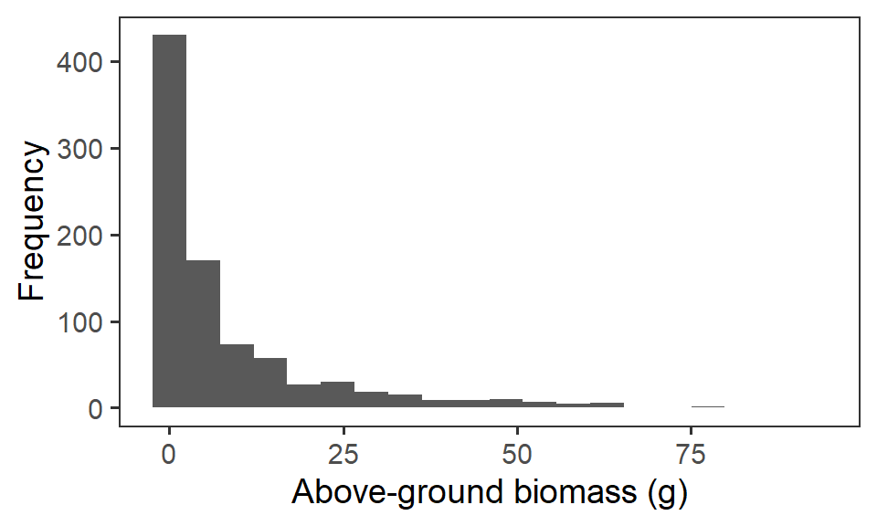
sessionInfo()R version 4.0.5 (2021-03-31)
Platform: x86_64-w64-mingw32/x64 (64-bit)
Running under: Windows 10 x64 (build 19042)
Matrix products: default
locale:
[1] LC_COLLATE=English_United Kingdom.1252
[2] LC_CTYPE=English_United Kingdom.1252
[3] LC_MONETARY=English_United Kingdom.1252
[4] LC_NUMERIC=C
[5] LC_TIME=English_United Kingdom.1252
attached base packages:
[1] stats graphics grDevices utils datasets methods base
other attached packages:
[1] tidybayes_2.3.1 brms_2.15.0 Rcpp_1.0.6 vegan_2.5-7
[5] lattice_0.20-41 permute_0.9-5 patchwork_1.1.1 forcats_0.5.1
[9] stringr_1.4.0 dplyr_1.0.5 purrr_0.3.4 readr_1.4.0
[13] tidyr_1.1.3 tibble_3.1.0 ggplot2_3.3.3 tidyverse_1.3.0
loaded via a namespace (and not attached):
[1] readxl_1.3.1 backports_1.2.1 workflowr_1.6.2
[4] plyr_1.8.6 igraph_1.2.6 splines_4.0.5
[7] svUnit_1.0.3 crosstalk_1.1.1 rstantools_2.1.1
[10] inline_0.3.17 digest_0.6.27 htmltools_0.5.1.1
[13] rsconnect_0.8.16 fansi_0.4.2 magrittr_2.0.1
[16] cluster_2.1.1 modelr_0.1.8 RcppParallel_5.0.3
[19] matrixStats_0.58.0 xts_0.12.1 prettyunits_1.1.1
[22] colorspace_2.0-0 rvest_1.0.0 ggdist_2.4.0
[25] haven_2.3.1 xfun_0.22 callr_3.6.0
[28] crayon_1.4.1 jsonlite_1.7.2 lme4_1.1-26
[31] zoo_1.8-9 glue_1.4.2 gtable_0.3.0
[34] emmeans_1.6.0 V8_3.4.0 distributional_0.2.2
[37] pkgbuild_1.2.0 rstan_2.21.2 abind_1.4-5
[40] scales_1.1.1 mvtnorm_1.1-1 DBI_1.1.1
[43] miniUI_0.1.1.1 xtable_1.8-4 stats4_4.0.5
[46] StanHeaders_2.21.0-7 DT_0.17 htmlwidgets_1.5.3
[49] httr_1.4.2 threejs_0.3.3 arrayhelpers_1.1-0
[52] ellipsis_0.3.1 farver_2.1.0 pkgconfig_2.0.3
[55] loo_2.4.1 sass_0.3.1 dbplyr_2.1.0
[58] utf8_1.2.1 labeling_0.4.2 tidyselect_1.1.0
[61] rlang_0.4.10 reshape2_1.4.4 later_1.1.0.1
[64] munsell_0.5.0 cellranger_1.1.0 tools_4.0.5
[67] cli_2.3.1 generics_0.1.0 broom_0.7.5
[70] ggridges_0.5.3 evaluate_0.14 fastmap_1.1.0
[73] yaml_2.2.1 processx_3.5.0 knitr_1.31
[76] fs_1.5.0 nlme_3.1-152 whisker_0.4
[79] mime_0.10 projpred_2.0.2 xml2_1.3.2
[82] compiler_4.0.5 bayesplot_1.8.0 shinythemes_1.2.0
[85] rstudioapi_0.13 gamm4_0.2-6 curl_4.3
[88] reprex_2.0.0 statmod_1.4.35 bslib_0.2.4
[91] stringi_1.5.3 highr_0.8 ps_1.6.0
[94] Brobdingnag_1.2-6 Matrix_1.3-2 nloptr_1.2.2.2
[97] markdown_1.1 shinyjs_2.0.0 vctrs_0.3.7
[100] pillar_1.5.1 lifecycle_1.0.0 jquerylib_0.1.3
[103] bridgesampling_1.0-0 estimability_1.3 httpuv_1.5.5
[106] R6_2.5.0 promises_1.2.0.1 gridExtra_2.3
[109] codetools_0.2-18 boot_1.3-27 colourpicker_1.1.0
[112] MASS_7.3-53.1 gtools_3.8.2 assertthat_0.2.1
[115] rprojroot_2.0.2 withr_2.4.1 shinystan_2.5.0
[118] mgcv_1.8-34 parallel_4.0.5 hms_1.0.0
[121] grid_4.0.5 coda_0.19-4 minqa_1.2.4
[124] rmarkdown_2.7 git2r_0.28.0 shiny_1.6.0
[127] lubridate_1.7.10 base64enc_0.1-3 dygraphs_1.1.1.6