Session 07 - Exercises Key
Last updated: 2023-07-24
Checks: 7 0
Knit directory:
SISG2023_Association_Mapping/
This reproducible R Markdown analysis was created with workflowr (version 1.7.0). The Checks tab describes the reproducibility checks that were applied when the results were created. The Past versions tab lists the development history.
Great! Since the R Markdown file has been committed to the Git repository, you know the exact version of the code that produced these results.
Great job! The global environment was empty. Objects defined in the global environment can affect the analysis in your R Markdown file in unknown ways. For reproduciblity it’s best to always run the code in an empty environment.
The command set.seed(20230530) was run prior to running
the code in the R Markdown file. Setting a seed ensures that any results
that rely on randomness, e.g. subsampling or permutations, are
reproducible.
Great job! Recording the operating system, R version, and package versions is critical for reproducibility.
Nice! There were no cached chunks for this analysis, so you can be confident that you successfully produced the results during this run.
Great job! Using relative paths to the files within your workflowr project makes it easier to run your code on other machines.
Great! You are using Git for version control. Tracking code development and connecting the code version to the results is critical for reproducibility.
The results in this page were generated with repository version 6eed1d7. See the Past versions tab to see a history of the changes made to the R Markdown and HTML files.
Note that you need to be careful to ensure that all relevant files for
the analysis have been committed to Git prior to generating the results
(you can use wflow_publish or
wflow_git_commit). workflowr only checks the R Markdown
file, but you know if there are other scripts or data files that it
depends on. Below is the status of the Git repository when the results
were generated:
Untracked files:
    Untracked:  analysis/SISGM15_prac5Solution.Rmd
    Untracked:  analysis/SISGM15_prac6Solution.Rmd
    Untracked:  analysis/SISGM15_prac9Solution.Rmd
    Untracked:  analysis/Session08_practical_Key.Rmd
Note that any generated files, e.g. HTML, png, CSS, etc., are not included in this status report because it is ok for generated content to have uncommitted changes.
These are the previous versions of the repository in which changes were
made to the R Markdown
(analysis/Session07_practical_Key.Rmd) and HTML
(docs/Session07_practical_Key.html) files. If you’ve
configured a remote Git repository (see ?wflow_git_remote),
click on the hyperlinks in the table below to view the files as they
were in that past version.
| File | Version | Author | Date | Message |
|---|---|---|---|---|
| Rmd | 6eed1d7 | Joelle Mbatchou | 2023-07-24 | update s7 key |
Before you begin:
- Make sure that R is installed on your computer
- For this lab, we will use the following R libraries:
library(data.table)
library(dplyr)
library(tidyr)
library(BEDMatrix)
library(SKAT)
library(ACAT)
library(ggplot2)
Rare Variant Analysis
Introduction
We will look into a dataset collected on a quantitative phenotype which was first analyzed through GWAS and a signal was detected in chromosome 1. Let’s determine whether the signal is present when we focus on rare variation at the locus. In our analyses, we will define rare variants as those with \(MAF \leq 5\%\).
The file “rv_pheno.txt”” contains the phenotype measurements for a set of individuals and the file “rv_geno_chr1.bed” is a binary file in PLINK BED format with accompanying BIM and FAM files which contains the genotype data.
Exercises
Here are some things to try:
- Using PLINK, extract rare variants in a new PLINK BED file.
system("/data/SISG2023M15/exe/plink2 --bfile /data/SISG2023M15/data/rv_geno_chr1 --max-maf 0.05 --maj-ref force --make-bed --out chr1_region_rv")- Load the data in R:
- Read in the SNPs using R function
BEDMatrix()
G <- BEDMatrix("chr1_region_rv", simple_names = TRUE)Extracting number of samples and rownames from chr1_region_rv.fam...Extracting number of variants and colnames from chr1_region_rv.bim...- Load the phenotype data from
rv_pheno.txt
y <- fread("/data/SISG2023M15/data/rv_pheno.txt", header = TRUE)- Keep only samples who are present both in the genotype as well as phenotype data and who don’t have missing values for the phenotype
ids.keep <- y %>% drop_na(Pheno) %>% pull(IID)
length(ids.keep)
[1] 9949G <- G[match(ids.keep, rownames(G)), ]
y <- y %>% drop_na(Pheno)
dim(G)[1] 9949 56- Examine the genotype data:
- Compute the minor allele frequency (MAF) for each SNP and plot histogram.
maf <- apply(G, 2, function(x) mean(x, na.rm=TRUE))/2
maf %>% hist(xlab = "Minor allele frequencies", main = "Distribution of MAF")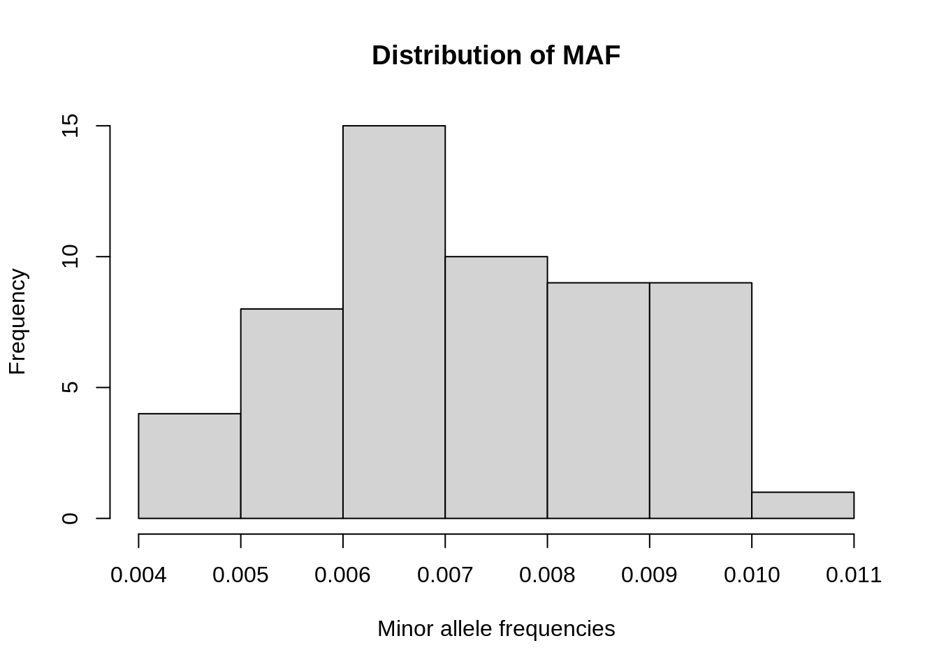
- Check for missing values.
sum(is.na(G))[1] 0- Run the single variant association tests in PLINK (only for the extracted variants).
system("/data/SISG2023M15/exe/plink2 --bfile chr1_region_rv --pheno /data/SISG2023M15/data/rv_pheno.txt --pheno-name Pheno --glm allow-no-covars --out sv_test")- What would be your significance threshold after applying Bonferroni correction for the multiple tests (assume the significance level is 0.05)? Is anything significant after this correction?
sv_pvals <- fread("sv_test.Pheno.glm.linear")
bonf.p <- 0.05 / length(sv_pvals$P)
bonf.p
[1] 0.0008928571sv_pvals[P <= bonf.p, ] %>%
arrange(P) #CHROM POS ID REF ALT PROVISIONAL_REF? A1 OMITTED
1: 1 12639385 1:12639385:G:A A G Y G A
2: 1 12057950 1:12057950:C:T T C Y C T
3: 1 12734720 1:12734720:A:C C A Y A C
4: 1 12405413 1:12405413:T:C C T Y T C
5: 1 12360016 1:12360016:G:A A G Y G A
6: 1 12183493 1:12183493:G:A A G Y G A
A1_FREQ TEST OBS_CT BETA SE T_STAT P ERRCODE
1: 0.00567896 ADD 9949 0.391421 0.0955243 4.09761 4.20759e-05 .
2: 0.00789024 ADD 9949 -0.323574 0.0801934 -4.03492 5.50288e-05 .
3: 0.00849332 ADD 9949 -0.278236 0.0769709 -3.61482 3.02042e-04 .
4: 0.00487486 ADD 9949 0.359249 0.1019850 3.52258 4.29282e-04 .
5: 0.00643281 ADD 9949 -0.310260 0.0898433 -3.45335 5.55975e-04 .
6: 0.00773947 ADD 9949 0.274311 0.0814842 3.36643 7.64368e-04 .- Make a volcano plot (i.e. log10 p-values vs effect sizes).
sv_pvals %>%
  ggplot(aes(x = sv_pvals$BETA, y = -log10(sv_pvals$P))) +
  geom_point() +
  labs(x = "Effect size", y = "-log10P")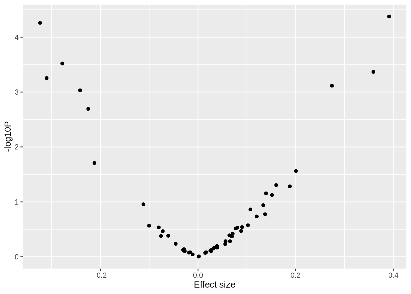
- We will first compare three collapsing/burden approaches:
- CAST (Binary collapsing approach): for each individual, count where they have a rare allele at any of the sites
- MZ Test/GRANVIL (Count based collapsing): for each individual, count the total number of sites where a rare allele is present
- Weighted burden test: for each individual, take a weighted count of
the rare alleles across sites (for the weights, use
weights <- dbeta(MAF, 1, 25))
For each approach, first generate the burden scores vector then test
it for association with the phenotype using lm() R
function.
# CAST
# count number of rare alleles for each person and determine if it is > 0
burden.cast <- as.numeric( apply(G, 1, sum) > 0 )
lm(y$Pheno ~ burden.cast) %>% summary
Call:
lm(formula = y$Pheno ~ burden.cast)

Residuals:
    Min      1Q  Median      3Q     Max
-3.9531 -0.6880  0.0012  0.6822  3.6581

Coefficients:
            Estimate Std. Error t value Pr(>|t|)
(Intercept) 0.002423   0.015317   0.158    0.874
burden.cast 0.017757   0.020422   0.870    0.385

Residual standard error: 1.01 on 9947 degrees of freedom
Multiple R-squared:  7.6e-05,   Adjusted R-squared:  -2.452e-05
F-statistic: 0.7561 on 1 and 9947 DF,  p-value: 0.3846
# MZ
# count number of sites with rare alleles for each person
burden.mz <- apply( G > 0 , 1, sum)
lm(y$Pheno ~ burden.mz) %>% summary
Call:
lm(formula = y$Pheno ~ burden.mz)

Residuals:
    Min      1Q  Median      3Q     Max
-3.9521 -0.6894 -0.0013  0.6805  3.6591

Coefficients:
            Estimate Std. Error t value Pr(>|t|)
(Intercept) 0.001444   0.013700   0.105    0.916
burden.mz   0.013492   0.011346   1.189    0.234

Residual standard error: 1.01 on 9947 degrees of freedom
Multiple R-squared:  0.0001421, Adjusted R-squared:  4.162e-05
F-statistic: 1.414 on 1 and 9947 DF,  p-value: 0.2344
# Weighted burden
# weighted sum of genotype counts across sites
weights <- dbeta(maf, 1, 25)
burden.weighted <- G %*% weights
lm(y$Pheno ~ burden.weighted) %>% summary
Call:
lm(formula = y$Pheno ~ burden.weighted)

Residuals:
    Min      1Q  Median      3Q     Max
-3.9519 -0.6896 -0.0014  0.6804  3.6593

Coefficients:
                 Estimate Std. Error t value Pr(>|t|)
(Intercept)     0.0012244  0.0136778   0.090    0.929
burden.weighted 0.0006577  0.0005402   1.217    0.223

Residual standard error: 1.01 on 9947 degrees of freedom
Multiple R-squared:  0.000149,  Adjusted R-squared:  4.846e-05
F-statistic: 1.482 on 1 and 9947 DF, p-value: 0.2235- Now use SKAT to test for an association.
# fit null model (no covariates)
skat.null <- SKAT_Null_Model(y$Pheno ~ 1 , out_type = "C")
# Run SKAT association test
SKAT(G, skat.null )$p.value
[1] 8.745405e-11- Run the omnibus SKAT, but consider setting \(\rho\) (i.e.
r.corr) to 0 and then 1.
- Compare the results to using the CAST,MZ/GRANVIL and Weighted burden collapsing approaches in Question 5 as well as SKAT in Question 6. What tests do these \(\rho\) values correspond to?
# Run SKATO association test specifying rho
p.skato.r0 <- SKAT(G, skat.null, r.corr = 0)$p.value
p.skato.r1 <- SKAT(G, skat.null, r.corr = 1)$p.value
c(rho0 = p.skato.r0, rho1 = p.skato.r1)
rho0 rho1
8.745405e-11 2.234603e-01 - Now the omnibus version of SKAT, but use the “optimal.adj” approach which searches across a range of rho values.
# Run SKATO association test using grid of rho values
SKAT(G, skat.null, method="optimal.adj")$p.value
[1] 6.121784e-10- Run ACATV on the single variant p-values.
# `weights` vector is from Qesution 5
acat.weights <- weights^2 * maf * (1 - maf)
p.acatv <- ACAT(sv_pvals$P, weights = acat.weights)
p.acatv
[1] 0.00112117- Run ACATO combining the SKAT and BURDEN p-values (from Question 7) with the ACATV p-value.
ACAT( c(p.skato.r0, p.skato.r1, p.acatv) )[1] 2.623621e-10
sessionInfo()R version 4.3.1 (2023-06-16)
Platform: x86_64-pc-linux-gnu (64-bit)
Running under: Ubuntu 22.04.2 LTS
Matrix products: default
BLAS: /usr/lib/x86_64-linux-gnu/blas/libblas.so.3.10.0
LAPACK: /usr/lib/x86_64-linux-gnu/lapack/liblapack.so.3.10.0
locale:
[1] LC_CTYPE=C.UTF-8 LC_NUMERIC=C LC_TIME=C.UTF-8
[4] LC_COLLATE=C.UTF-8 LC_MONETARY=C.UTF-8 LC_MESSAGES=C.UTF-8
[7] LC_PAPER=C.UTF-8 LC_NAME=C LC_ADDRESS=C
[10] LC_TELEPHONE=C LC_MEASUREMENT=C.UTF-8 LC_IDENTIFICATION=C
time zone: Etc/UTC
tzcode source: system (glibc)
attached base packages:
[1] stats graphics grDevices utils datasets methods base
other attached packages:
[1] ggplot2_3.4.2 ACAT_0.91 SKAT_2.2.5 RSpectra_0.16-1
[5] SPAtest_3.1.2 Matrix_1.5-4.1 BEDMatrix_2.0.3 tidyr_1.3.0
[9] dplyr_1.1.2 data.table_1.14.8
loaded via a namespace (and not attached):
[1] sass_0.4.6 utf8_1.2.3 generics_0.1.3 stringi_1.7.12
[5] lattice_0.21-8 digest_0.6.33 magrittr_2.0.3 evaluate_0.21
[9] grid_4.3.1 fastmap_1.1.1 rprojroot_2.0.3 workflowr_1.7.0
[13] jsonlite_1.8.7 whisker_0.4.1 promises_1.2.0.1 purrr_1.0.1
[17] fansi_1.0.4 scales_1.2.1 jquerylib_0.1.4 cli_3.6.1
[21] rlang_1.1.1 munsell_0.5.0 withr_2.5.0 cachem_1.0.8
[25] yaml_2.3.7 tools_4.3.1 colorspace_2.1-0 httpuv_1.6.11
[29] crochet_2.3.0 vctrs_0.6.3 R6_2.5.1 lifecycle_1.0.3
[33] git2r_0.32.0 stringr_1.5.0 fs_1.6.2 pkgconfig_2.0.3
[37] pillar_1.9.0 bslib_0.5.0 later_1.3.1 gtable_0.3.3
[41] glue_1.6.2 Rcpp_1.0.11 highr_0.10 xfun_0.39
[45] tibble_3.2.1 tidyselect_1.2.0 rstudioapi_0.15.0 knitr_1.43
[49] farver_2.1.1 htmltools_0.5.5 labeling_0.4.2 rmarkdown_2.23
[53] compiler_4.3.1