Session 02 - Exercises Key
Last updated: 2023-07-24
Checks: 7 0
Knit directory:
SISG2023_Association_Mapping/
This reproducible R Markdown analysis was created with workflowr (version 1.7.0). The Checks tab describes the reproducibility checks that were applied when the results were created. The Past versions tab lists the development history.
Great! Since the R Markdown file has been committed to the Git repository, you know the exact version of the code that produced these results.
Great job! The global environment was empty. Objects defined in the global environment can affect the analysis in your R Markdown file in unknown ways. For reproduciblity it’s best to always run the code in an empty environment.
The command set.seed(20230530) was run prior to running
the code in the R Markdown file. Setting a seed ensures that any results
that rely on randomness, e.g. subsampling or permutations, are
reproducible.
Great job! Recording the operating system, R version, and package versions is critical for reproducibility.
Nice! There were no cached chunks for this analysis, so you can be confident that you successfully produced the results during this run.
Great job! Using relative paths to the files within your workflowr project makes it easier to run your code on other machines.
Great! You are using Git for version control. Tracking code development and connecting the code version to the results is critical for reproducibility.
The results in this page were generated with repository version d47504f. See the Past versions tab to see a history of the changes made to the R Markdown and HTML files.
Note that you need to be careful to ensure that all relevant files for
the analysis have been committed to Git prior to generating the results
(you can use wflow_publish or
wflow_git_commit). workflowr only checks the R Markdown
file, but you know if there are other scripts or data files that it
depends on. Below is the status of the Git repository when the results
were generated:
Untracked files:
    Untracked:  analysis/SISGM15_prac5Solution.Rmd
    Untracked:  analysis/SISGM15_prac6Solution.Rmd
    Untracked:  analysis/SISGM15_prac9Solution.Rmd
    Untracked:  analysis/Session01_practical_Key.Rmd
    Untracked:  analysis/Session07_practical_Key.Rmd
    Untracked:  analysis/Session08_practical_Key.Rmd
Note that any generated files, e.g. HTML, png, CSS, etc., are not included in this status report because it is ok for generated content to have uncommitted changes.
These are the previous versions of the repository in which changes were
made to the R Markdown
(analysis/Session02_practical_Key.Rmd) and HTML
(docs/Session02_practical_Key.html) files. If you’ve
configured a remote Git repository (see ?wflow_git_remote),
click on the hyperlinks in the table below to view the files as they
were in that past version.
| File | Version | Author | Date | Message |
|---|---|---|---|---|
| Rmd | d47504f | Joelle Mbatchou | 2023-07-24 | add session 2 key |
| html | 532fb30 | Joelle Mbatchou | 2023-07-24 | update doc |
| html | dea7629 | Joelle Mbatchou | 2023-07-24 | add key to website |
Before you begin:
- Make sure that R is installed on your computer
- For this lab, we will use the following R libraries:
library(data.table)
library(dplyr)
library(tidyr)
library(bigsnpr)
library(ggplot2)
Population Structure Inference
Introduction
We will be working with a subset of the genotype data from the Human Genome Diversity Panel (HGDP) and HapMap.
The file “YRI_CEU_ASW_MEX_NAM.bed” is a binary file in PLINK BED format with accompanying BIM and FAM files. It contains genotype data at autosomal SNPs for:
- Native American samples from HGDP (NAM)
- Four population samples from HapMap:
- Yoruba in Ibadan, Nigeria (YRI)
- Utah residents with ancestry from Northern and Western Europe (CEU)
- Mexican Americans in Los Angeles, California (MXL)
- African Americans from the south-western United States (ASW)
Exercises
Here are some things to look at:
- Examine the dataset:
- How many samples are present?
famfile <- fread("/data/SISG2023M15/data/YRI_CEU_ASW_MEX_NAM.fam", header = FALSE)
famfile %>% head
V1 V2 V3 V4 V5 V6
1: 1432 HGDP00702 0 0 2 -9
2: 1433 HGDP00703 0 0 1 -9
3: 1434 HGDP00704 0 0 2 -9
4: 1436 HGDP00706 0 0 2 -9
5: 1438 HGDP00708 0 0 2 -9
6: 1440 HGDP00710 0 0 1 -9famfile %>% nrow[1] 604- How many SNPs?
bimfile <- fread("/data/SISG2023M15/data/YRI_CEU_ASW_MEX_NAM.bim", header = FALSE)
bimfile %>% head
V1 V2 V3 V4 V5 V6
1: 1 rs9442372 0 1008567 1 2
2: 1 rs2887286 0 1145994 1 2
3: 1 rs3813199 0 1148140 1 2
4: 1 rs6685064 0 1201155 1 2
5: 1 rs9439462 0 1452629 1 2
6: 1 rs3820011 0 1878053 1 2bimfile %>% nrow[1] 150872- What is the number of samples in each population?
pop_info <- fread("/data/SISG2023M15/data/Population_Sample_Info.txt", header = TRUE)
head(pop_info)
FID IID Population
1: 1432 HGDP00702 NAM
2: 1433 HGDP00703 NAM
3: 1434 HGDP00704 NAM
4: 1436 HGDP00706 NAM
5: 1438 HGDP00708 NAM
6: 1440 HGDP00710 NAM# join with fam file
fam_pop_info <- left_join(famfile, pop_info, by = c("V1" = "FID", "V2" = "IID"))
fam_pop_info %>% select(Population) %>% tablePopulation
ASW CEU MXL NAM YRI
87 165 86 63 203 - Get the first 10 principal components (PCs) in PLINK using all SNPs.
system("/data/SISG2023M15/exe/plink2 --bfile /data/SISG2023M15/data/YRI_CEU_ASW_MEX_NAM --pca 10 --out pca_out")- Make a scatterplot of the first two PCs with each point colored by population membership.
pcs <- left_join(fam_pop_info, fread("pca_out.eigenvec"), by = c("V1" = "#FID", "V2" = "IID"))
pcs %>%
  ggplot(aes(x=PC1, y=PC2, color = Population)) +
  geom_point()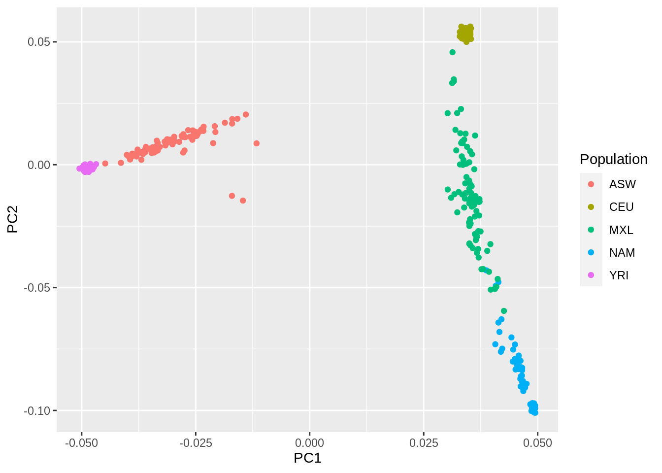
- Interpret the first two PCs, what ancestries are they reflecting?
- Make a scree plot of the eigenvalues for the first 10 PCs. Approximate the proportion of variance explained by the first two PCs.
evals.pca <- fread("pca_out.eigenval", header = FALSE)
evals.pca %>%
  ggplot(aes(x = 1:10, y = V1)) +
  geom_point() +
  geom_line() +
  scale_x_continuous(breaks = 1:10) +
  labs(x = "PC", y = "Eigenvalue")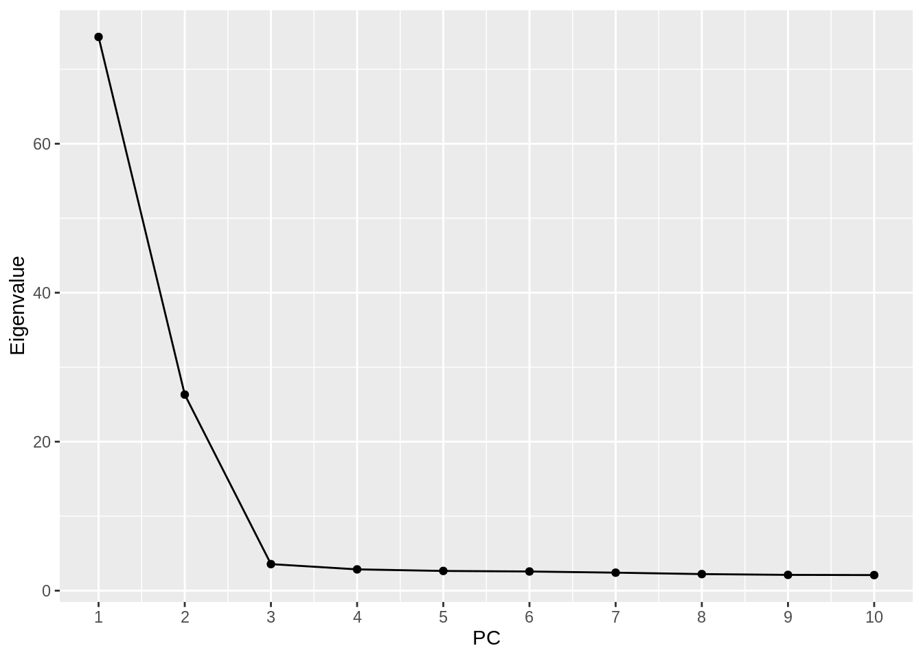
sum(evals.pca$V1[1:2]) / sum(evals.pca$V1)[1] 0.8308752- Now redo Question 2 above using the
bigsnprR package specifying a \(r^2\) threshold of 0.2 (i.e. LD pruning) as well as a minimum minor allele count (MAC) of 20.
- Run PCA and make a scatter plot of the first two principal components (PCs) with each point colored according to population membership.
obj.bed <- bed(bedfile = "/data/SISG2023M15/data/YRI_CEU_ASW_MEX_NAM.bed")
pca.bigsnpr <- bed_autoSVD(
  obj.bed,
  thr.r2 = 0.2,
  k = 10,
  min.mac = 20
)
Phase of clumping (on MAC) at r^2 > 0.2.. keep 87127 variants.
Discarding 48 variants with MAC < 20.

Iteration 1:
Computing SVD..
The default of 'doScale' is FALSE now for stability;
set options(mc_doScale_quiet=TRUE) to suppress this (once per session) message0 outlier variant detected..
Converged!plot(pca.bigsnpr, type = "scores", scores = 1:2) +
aes(color = fam_pop_info$Population) +
labs(color = "Population")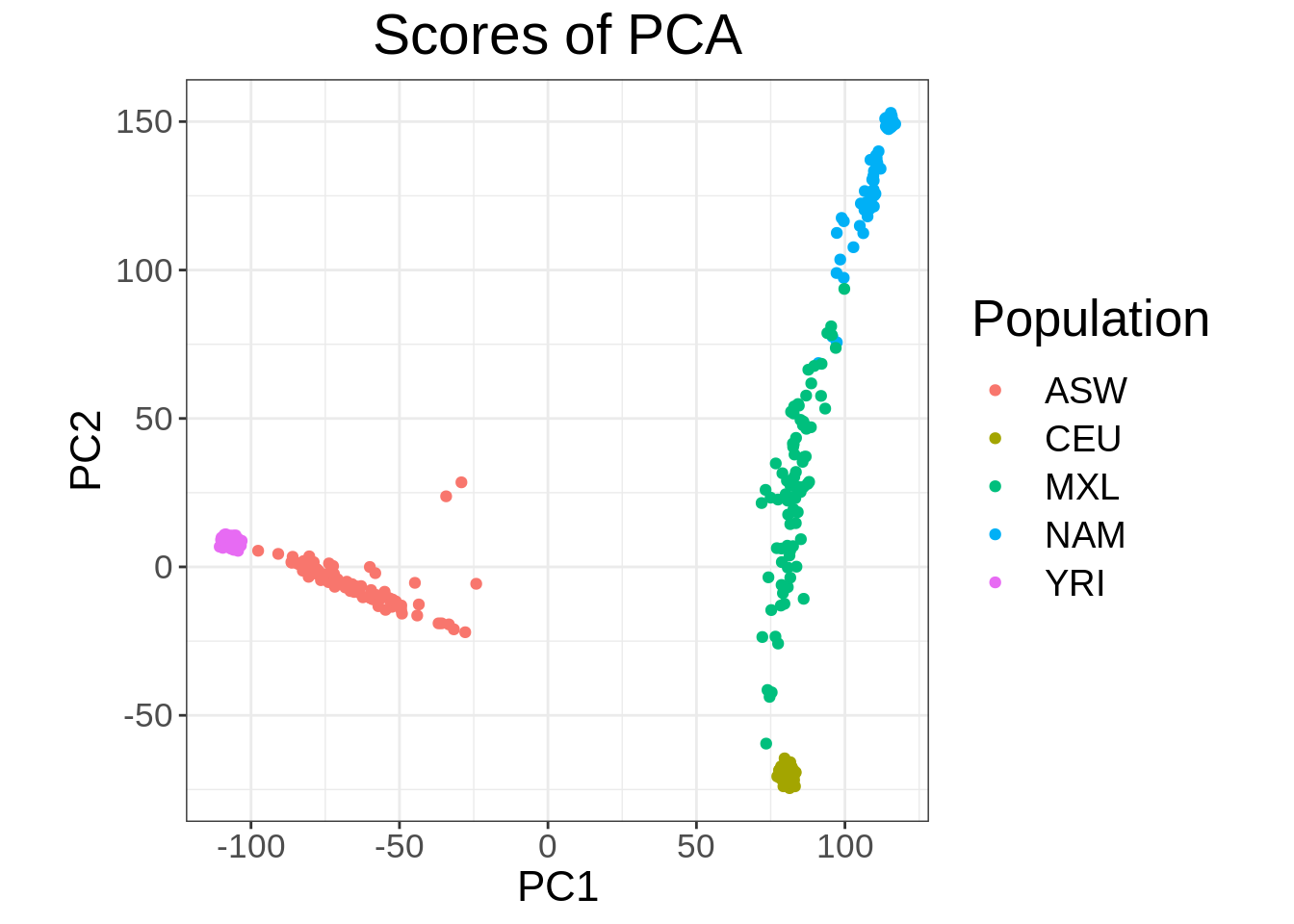
- Does the plot change from the one in Question 2?
- Check the SNP loadings for the first 10 PCs.
plot(pca.bigsnpr, type = "loadings", loadings = 1:10, coeff = 0.4)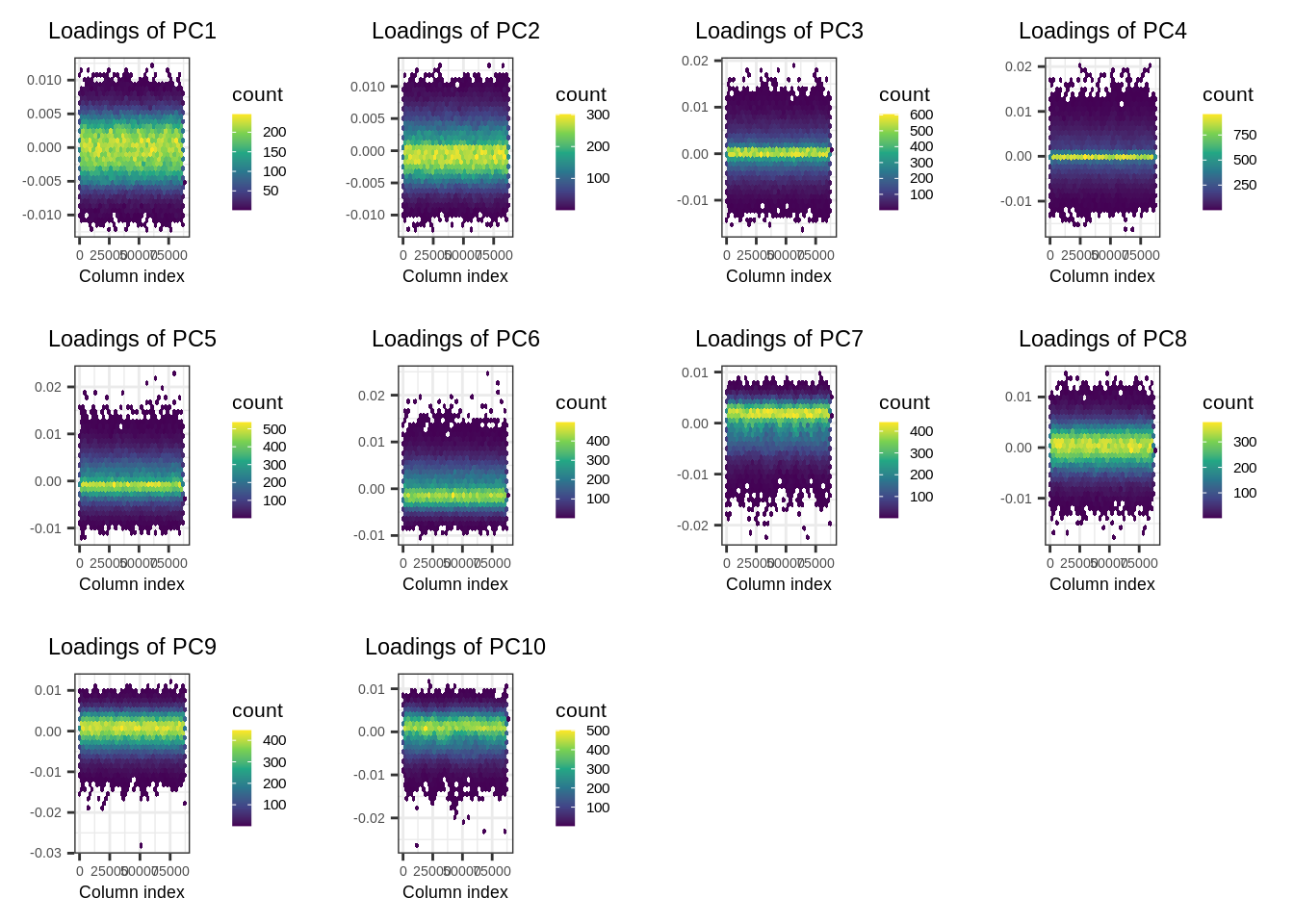
- Predict proportional Native American and European Ancestry for the HapMap MXL from the PCA output in Question 3 using one of the principal components. (Which PC is most appropriate for this analysis?) Assume that the HapMap MXL have negligible African Ancestry.
pca.bigsnpr %>% strList of 7
$ d : num [1:10] 2262 1434 553 495 474 ...
$ u : num [1:604, 1:10] 0.0488 0.043 0.0489 0.0489 0.0492 ...
$ v : num [1:87079, 1:10] -0.00229 -0.00165 -0.00315 -0.00888 0.00177 ...
$ niter : num 7
$ nops : num 128
$ center: num [1:87079] 0.818 0.914 0.233 0.827 0.432 ...
$ scale : num [1:87079] 0.695 0.704 0.454 0.696 0.582 ...
- attr(*, "class")= chr "big_SVD"
- attr(*, "subset")= int [1:87079] 1 2 3 5 6 8 10 11 12 13 ...
- attr(*, "lrldr")='data.frame': 0 obs. of 3 variables:
..$ Chr : int(0)
..$ Start: int(0)
..$ Stop : int(0) ceu.mean <- pca.bigsnpr$u[fam_pop_info$Population == "CEU",2] %>% mean
nam.mean <- pca.bigsnpr$u[fam_pop_info$Population == "NAM",2] %>% mean
c(ceu.mean, nam.mean)[1] -0.04885356 0.09084845mxl.prop.nam <- (pca.bigsnpr$u[fam_pop_info$Population == "MXL",2] - ceu.mean) / abs(nam.mean - ceu.mean)
mxl.prop.nam %>% summary Min. 1st Qu. Median Mean 3rd Qu. Max.
0.05262 0.37780 0.48238 0.47152 0.58381 0.81709 - Make a barplot of the proportional ancestry estimates from question 4.
data.frame(
ind = 1:length(mxl.prop.nam),
NAM = sort(mxl.prop.nam, decreasing = TRUE)
) %>%
mutate(CEU = 1 - NAM) %>%
gather(Pop, Prop, NAM, CEU) %>%
ggplot(aes(x = ind, y = Prop, fill = factor(Pop, levels = c("NAM", "CEU")))) +
geom_bar(position="stack", stat="identity") +
labs(x="Sample", y = "Ancestry Proportion", fill = "Population")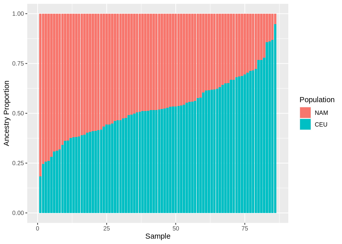
- Check if there are samples related 2nd degree or closer. If so, run PCA as in Question 3 removing these samples then project the remaining samples onto the PC space.
# check for 2nd degree relateds or closer
rel.df <- snp_plinkKINGQC(
plink2.path = "/data/SISG2023M15/exe/plink2",
bedfile.in = "/data/SISG2023M15/data/YRI_CEU_ASW_MEX_NAM.bed",
thr.king = 2^-3.5,
make.bed = FALSE
)
rel.df %>% str'data.frame': 362 obs. of 8 variables:
$ FID1 : chr "1563" "1567" "1567" "1570" ...
$ IID1 : chr "HGDP00845" "HGDP00849" "HGDP00849" "HGDP00852" ...
$ FID2 : chr "1556" "1556" "1561" "1551" ...
$ IID2 : chr "HGDP00838" "HGDP00838" "HGDP00843" "HGDP00832" ...
$ NSNP : int 150801 150802 150832 150816 150822 150814 150819 150815 150674 150796 ...
$ HETHET : num 0.0976 0.1069 0.1059 0.099 0.1022 ...
$ IBS0 : num 0.0221 0.0219 0.0223 0.0219 0.0227 ...
$ KINSHIP: num 0.104 0.126 0.13 0.118 0.118 ...# Gets indices of samples not related (match by fid/iid)
rel.ids <- c(paste(rel.df$FID1, rel.df$IID1), paste(rel.df$FID2, rel.df$IID2))
indices.unrel <- which(!(paste(famfile$V1,famfile$V2) %in% rel.ids))
indices.unrel %>% str int [1:116] 1 2 3 4 5 6 8 12 15 16 ...# Run PCA excluding relateds
pca.bigsnpr.norels <- bed_autoSVD(
obj.bed,
ind.row = indices.unrel,
thr.r2 = 0.2,
k = 10,
min.mac = 20
)
Phase of clumping (on MAC) at r^2 > 0.2.. keep 77173 variants.
Discarding 12226 variants with MAC < 20.
Iteration 1:
Computing SVD..
0 outlier variant detected..

Converged!# Project related samples
PCs <- matrix(NA, nrow(obj.bed), ncol(pca.bigsnpr.norels$u))
PCs[indices.unrel, ] <- predict(pca.bigsnpr.norels) # pc from model (unrels)
proj.rels <- bed_projectSelfPCA(
pca.bigsnpr.norels,
obj.bed,
ind.row = (1:nrow(famfile))[-indices.unrel]
)
PCs[-indices.unrel, ] <- proj.rels$OADP_proj # pc from projection (rels)
data.frame(PC1 = PCs[,1], PC2 = PCs[,2], pop = fam_pop_info$Population, Type = c("Projected", "Model")[1 + (1:nrow(famfile)) %in% indices.unrel]) %>%
ggplot(aes(x = PC1, y = PC2, color = pop, shape = Type)) +
geom_point() +
labs(color = "Population")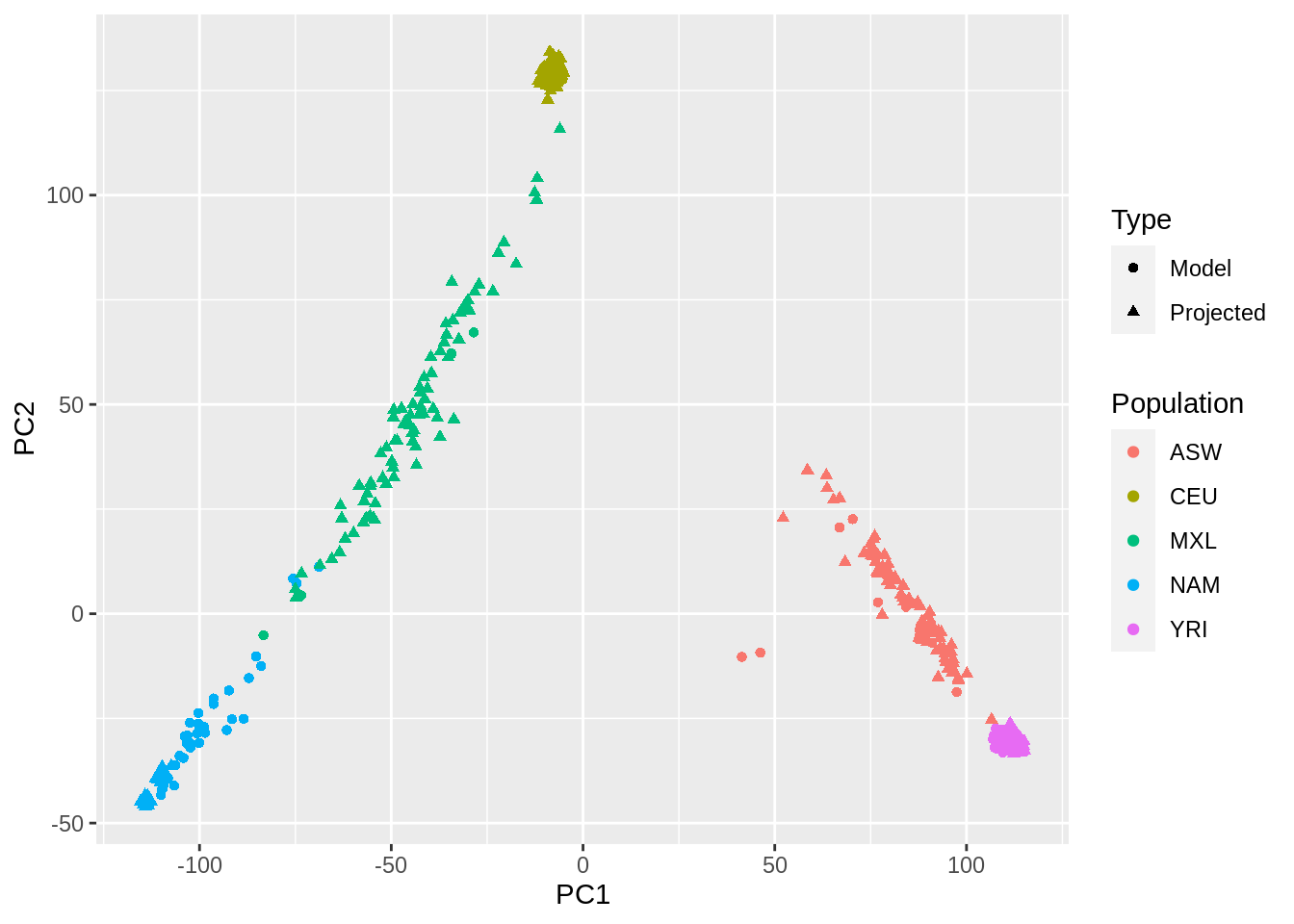
sessionInfo()R version 4.3.1 (2023-06-16)
Platform: x86_64-pc-linux-gnu (64-bit)
Running under: Ubuntu 22.04.2 LTS
Matrix products: default
BLAS: /usr/lib/x86_64-linux-gnu/blas/libblas.so.3.10.0
LAPACK: /usr/lib/x86_64-linux-gnu/lapack/liblapack.so.3.10.0
locale:
[1] LC_CTYPE=C.UTF-8 LC_NUMERIC=C LC_TIME=C.UTF-8
[4] LC_COLLATE=C.UTF-8 LC_MONETARY=C.UTF-8 LC_MESSAGES=C.UTF-8
[7] LC_PAPER=C.UTF-8 LC_NAME=C LC_ADDRESS=C
[10] LC_TELEPHONE=C LC_MEASUREMENT=C.UTF-8 LC_IDENTIFICATION=C
time zone: Etc/UTC
tzcode source: system (glibc)
attached base packages:
[1] stats graphics grDevices utils datasets methods base
other attached packages:
[1] ggplot2_3.4.2 bigsnpr_1.12.2 bigstatsr_1.5.12 tidyr_1.3.0
[5] dplyr_1.1.2 data.table_1.14.8
loaded via a namespace (and not attached):
[1] gtable_0.3.3 xfun_0.39 bslib_0.5.0 lattice_0.21-8
[5] bigassertr_0.1.6 vctrs_0.6.3 tools_4.3.1 ps_1.7.5
[9] generics_0.1.3 parallel_4.3.1 tibble_3.2.1 fansi_1.0.4
[13] DEoptimR_1.1-0 highr_0.10 pkgconfig_2.0.3 Matrix_1.5-4.1
[17] rngtools_1.5.2 lifecycle_1.0.3 compiler_4.3.1 farver_2.1.1
[21] stringr_1.5.0 git2r_0.32.0 munsell_0.5.0 bigparallelr_0.3.2
[25] codetools_0.2-19 httpuv_1.6.11 htmltools_0.5.5 sass_0.4.6
[29] yaml_2.3.7 hexbin_1.28.3 later_1.3.1 pillar_1.9.0
[33] jquerylib_0.1.4 whisker_0.4.1 cachem_1.0.8 doRNG_1.8.6
[37] iterators_1.0.14 foreach_1.5.2 robustbase_0.99-0 RSpectra_0.16-1
[41] parallelly_1.36.0 tidyselect_1.2.0 digest_0.6.33 stringi_1.7.12
[45] purrr_1.0.1 labeling_0.4.2 cowplot_1.1.1 rprojroot_2.0.3
[49] fastmap_1.1.1 grid_4.3.1 colorspace_2.1-0 cli_3.6.1
[53] magrittr_2.0.3 utf8_1.2.3 bigutilsr_0.3.4 withr_2.5.0
[57] scales_1.2.1 promises_1.2.0.1 rmarkdown_2.23 bigsparser_0.6.1
[61] rmio_0.4.0 bit_4.0.5 bigreadr_0.2.5 workflowr_1.7.0
[65] evaluate_0.21 ff_4.0.9 knitr_1.43 doParallel_1.0.17
[69] viridisLite_0.4.2 rlang_1.1.1 Rcpp_1.0.11 glue_1.6.2
[73] rstudioapi_0.15.0 jsonlite_1.8.7 R6_2.5.1 fs_1.6.2
[77] flock_0.7