Session 03 - Exercises Key
Last updated: 2023-07-24
Checks: 7 0
Knit directory:
SISG2023_Association_Mapping/
This reproducible R Markdown analysis was created with workflowr (version 1.7.0). The Checks tab describes the reproducibility checks that were applied when the results were created. The Past versions tab lists the development history.
Great! Since the R Markdown file has been committed to the Git repository, you know the exact version of the code that produced these results.
Great job! The global environment was empty. Objects defined in the global environment can affect the analysis in your R Markdown file in unknown ways. For reproduciblity it’s best to always run the code in an empty environment.
The command set.seed(20230530) was run prior to running
the code in the R Markdown file. Setting a seed ensures that any results
that rely on randomness, e.g. subsampling or permutations, are
reproducible.
Great job! Recording the operating system, R version, and package versions is critical for reproducibility.
Nice! There were no cached chunks for this analysis, so you can be confident that you successfully produced the results during this run.
Great job! Using relative paths to the files within your workflowr project makes it easier to run your code on other machines.
Great! You are using Git for version control. Tracking code development and connecting the code version to the results is critical for reproducibility.
The results in this page were generated with repository version 0afa232. See the Past versions tab to see a history of the changes made to the R Markdown and HTML files.
Note that you need to be careful to ensure that all relevant files for
the analysis have been committed to Git prior to generating the results
(you can use wflow_publish or
wflow_git_commit). workflowr only checks the R Markdown
file, but you know if there are other scripts or data files that it
depends on. Below is the status of the Git repository when the results
were generated:
Untracked files:
    Untracked:  analysis/SISGM15_prac4Solution.Rmd
    Untracked:  analysis/SISGM15_prac5Solution.Rmd
    Untracked:  analysis/SISGM15_prac6Solution.Rmd
    Untracked:  analysis/SISGM15_prac9Solution.Rmd
    Untracked:  analysis/Session01_practical_Key.Rmd
    Untracked:  analysis/Session02_practical_Key.Rmd
    Untracked:  analysis/Session07_practical_Key.Rmd
    Untracked:  analysis/Session08_practical_Key.Rmd
Note that any generated files, e.g. HTML, png, CSS, etc., are not included in this status report because it is ok for generated content to have uncommitted changes.
These are the previous versions of the repository in which changes were
made to the R Markdown
(analysis/Session03_practical_Key.Rmd) and HTML
(docs/Session03_practical_Key.html) files. If you’ve
configured a remote Git repository (see ?wflow_git_remote),
click on the hyperlinks in the table below to view the files as they
were in that past version.
| File | Version | Author | Date | Message |
|---|---|---|---|---|
| Rmd | 0afa232 | Joelle Mbatchou | 2023-07-24 | session 3 key |
Before you begin:
- Make sure that R is installed on your computer
- For this lab, we will use the following R libraries:
library(data.table)
library(dplyr)
library(tidyr)
library(GWASTools)
library(ggplot2)
GWAS in Samples with Structure
Introduction
We will be analyzing a simulated data set which contains sample structure to better understand the impact it can have in GWAS analyses if not accounted for. We will perform GWAS on a quantitative phenotype which was simulated to have high heritability and be highly polygenic.
The file “sim_rels_pheno.txt””
contains the phenotype measurements for a set of individuals and the
file “sim_rels_geno.bed” is a binary file in PLINK BED format with
accompanying BIM and FAM files which contains the genotype data
at null variants (i.e. simulated as not associated with
the phenotype).
How should we expect the QQ/Manhatthan plots to look like under this
scenario?
Exercises
Here are some things to try:
- Examine the dataset:
- How many samples are present?
famfile <- fread("/data/SISG2023M15/data/sim_rels_geno.fam", header = FALSE)
famfile %>% str
Classes 'data.table' and 'data.frame': 2400 obs. of 6 variables:
$ V1: int 2307 379 478 1545 990 1907 369 1694 2137 2314 ...
$ V2: int 2307 379 478 1545 990 1907 369 1694 2137 2314 ...
$ V3: int 0 0 0 0 0 0 0 0 0 0 ...
$ V4: int 0 0 0 0 0 0 0 0 0 0 ...
$ V5: int 1 2 1 1 1 2 2 1 2 1 ...
$ V6: int -9 -9 -9 -9 -9 -9 -9 -9 -9 -9 ...
- attr(*, ".internal.selfref")=<externalptr> - How many SNPs? In how many chromosomes?
bimfile <- fread("/data/SISG2023M15/data/sim_rels_geno.bim", header = FALSE)
bimfile %>% str
Classes 'data.table' and 'data.frame': 106134 obs. of 6 variables:
$ V1: int 1 1 1 1 1 1 1 1 1 1 ...
$ V2: chr "1:12000011:A:C" "1:12000012:A:C" "1:12000019:T:C" "1:12000027:C:T" ...
$ V3: int 0 0 0 0 0 0 0 0 0 0 ...
$ V4: int 12000011 12000012 12000019 12000027 12000036 12000061 12000073 12000074 12000117 12000136 ...
$ V5: chr "A" "A" "T" "C" ...
$ V6: chr "C" "C" "C" "T" ...
- attr(*, ".internal.selfref")=<externalptr> bimfile %>% select(V1) %>% tableV1
1 2 3 4 5 6 7 8 9 10 11 12 13 14 15 16
4918 4857 4813 4772 4810 4914 4840 4696 4790 4906 4782 4756 4803 4671 4814 4869
17 18 19 20 21 22
4632 4834 4908 4942 4947 4860 - Examine the phenotype data:
- How many individuals in the study have measurements?
yfile <- fread("/data/SISG2023M15/data/sim_rels_pheno.txt", header = TRUE)
yfile %>% str
Classes 'data.table' and 'data.frame': 2400 obs. of 3 variables:
$ FID : int 2307 379 478 1545 990 1907 369 1694 2137 2314 ...
$ IID : int 2307 379 478 1545 990 1907 369 1694 2137 2314 ...
$ Pheno: num 0.00999 -1.45253 0.11097 1.11363 -0.20993 ...
- attr(*, ".internal.selfref")=<externalptr> yfile %>% pull(Pheno) %>% is.na %>% table.
FALSE
2400 - Make a visual of the distribution of the phenotype?
yfile %>%
  ggplot(aes(x = Pheno)) +
  geom_histogram(colour="black", fill="white")
`stat_bin()` using `bins = 30`. Pick better value with `binwidth`.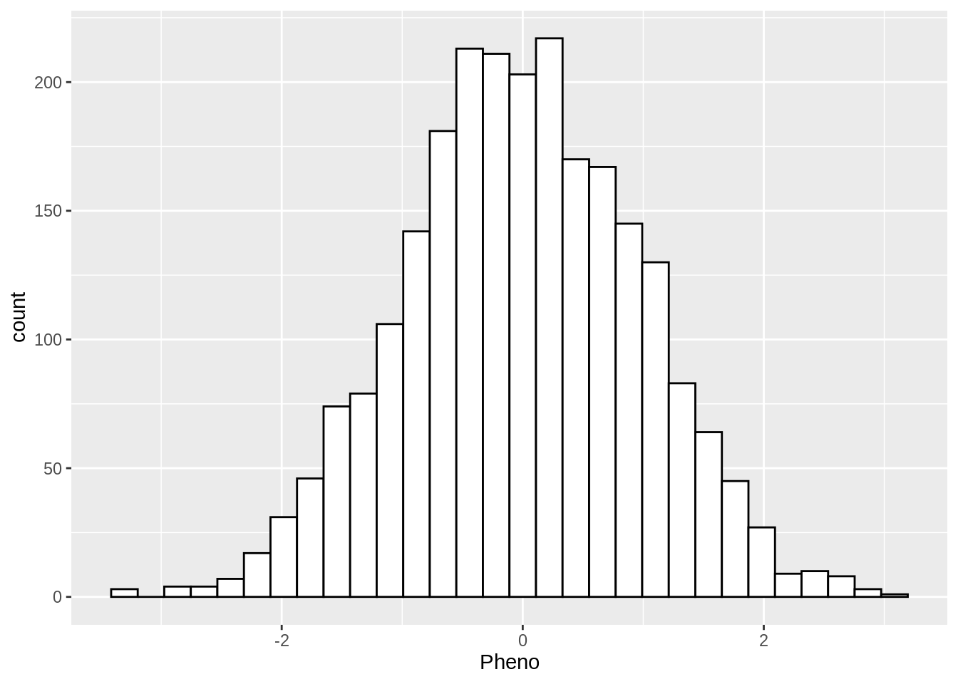
- Using PLINK, perform a GWAS using the phenotype file
sim_rels_pheno.txtand thesim_rels_geno.{bed,bim,fam}genotype files. Only perform association test on SNPs that pass the following quality control threshold filters:
- minor allele frequency (MAF) > 0.01
- at least a 99% genotyping call rate (less than 1% missing)
- HWE p-values greater than 0.001
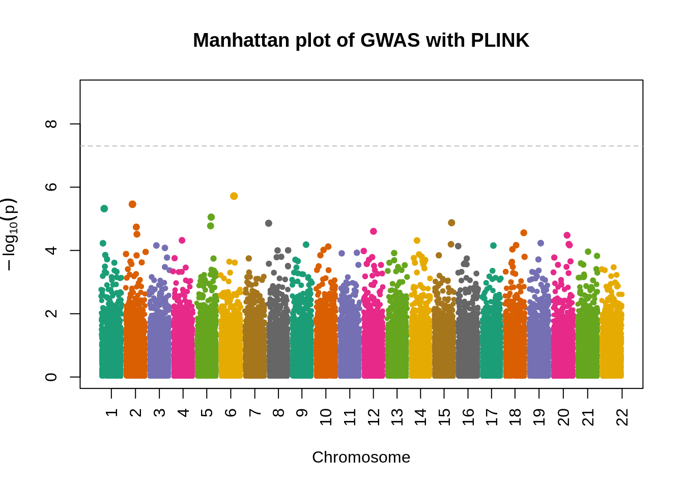
system("/data/SISG2023M15/exe/plink2 --bfile /data/SISG2023M15/data/sim_rels_geno --pheno /data/SISG2023M15/data/sim_rels_pheno.txt --pheno-name Pheno --maf 0.01 --geno 0.01 --hwe 0.001 --autosome --glm allow-no-covars --out gwas_plink")- Make a Manhattan plot of the association results using the
manhattanPlot()R function.
plink.gwas <- fread("gwas_plink.Pheno.glm.linear", header = TRUE)
plink.gwas %>% str
Classes 'data.table' and 'data.frame': 105886 obs. of 16 variables:
$ #CHROM : int 1 1 1 1 1 1 1 1 1 1 ...
$ POS : int 12000011 12000012 12000019 12000027 12000036 12000061 12000073 12000074 12000117 12000136 ...
$ ID : chr "1:12000011:A:C" "1:12000012:A:C" "1:12000019:T:C" "1:12000027:C:T" ...
$ REF : chr "C" "C" "C" "T" ...
$ ALT : chr "A" "A" "T" "C" ...
$ PROVISIONAL_REF?: chr "Y" "Y" "Y" "Y" ...
$ A1 : chr "A" "A" "T" "C" ...
$ OMITTED : chr "C" "C" "C" "T" ...
$ A1_FREQ : num 0.12 0.187 0.402 0.12 0.415 ...
$ TEST : chr "ADD" "ADD" "ADD" "ADD" ...
$ OBS_CT : int 2400 2400 2400 2400 2400 2400 2400 2400 2400 2400 ...
$ BETA : num 0.0122 -0.018 -0.0849 0.0125 0.0111 ...
$ SE : num 0.0438 0.0362 0.0284 0.0435 0.0288 ...
$ T_STAT : num 0.279 -0.497 -2.992 0.288 0.387 ...
$ P : num 0.78 0.6192 0.0028 0.7731 0.6991 ...
$ ERRCODE : chr "." "." "." "." ...
- attr(*, ".internal.selfref")=<externalptr> manhattanPlot(
p = plink.gwas$P,
chromosome = plink.gwas$`#CHROM`,
thinThreshold = 1e-4,
main= "Manhattan plot of GWAS with PLINK"
)
- Make a Q-Q plot of the association results using the
qqPlot()R function.
qqPlot(
  pval = plink.gwas$P,
  thinThreshold = 1e-4,
  main= "Q-Q plot of GWAS with PLINK"
 )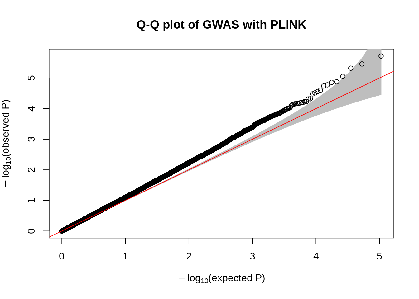
- Compute the genomic control inflation factor \(\lambda_{GC}\) based on the p-values. Is there evidence of possible inflation due to confounding?
chisq.stats <- qchisq(plink.gwas$P, df = 1, lower.tail = FALSE)
median(chisq.stats) / qchisq(0.5,1)
[1] 1.148451- Now use REGENIE to perform a GWAS of the phenotype using a whole genome regression model.
- We want to use high quality variants in the Step 1 null model fitting. Using PLINK, apply QC filters to remove variants with MAF below 5%, missingness above 1%, HWE p-value below 0.001, minor allele count (MAC) below 20.
system("/data/SISG2023M15/exe/plink2 --bfile /data/SISG2023M15/data/sim_rels_geno --maf 0.05 --geno 0.01 --hwe 0.001 --mac 20 --write-snplist --out qc_pass")- Run REGENIE Step 1 to fit the null model and obtain polygenic predictions using a leave-one-chromosome-out (LOCO) scheme
system("/data/SISG2023M15/exe/regenie --bed /data/SISG2023M15/data/sim_rels_geno --phenoFile /data/SISG2023M15/data/sim_rels_pheno.txt --step 1 --loocv --bsize 1000 --qt --extract qc_pass.snplist --out regenie_step1")The prediction list file output from Step 1 contains the path to the LOCO polygenic predictions:
fread("regenie_step1_pred.list", header = FALSE) V1 V2
1: Pheno /home/jmbatchou/regenie_step1_1.loco- Run REGENIE Step 2 to perform association testing at the same set of SNPs tested in PLINK.
plink.gwas %>%
select(ID) %>%
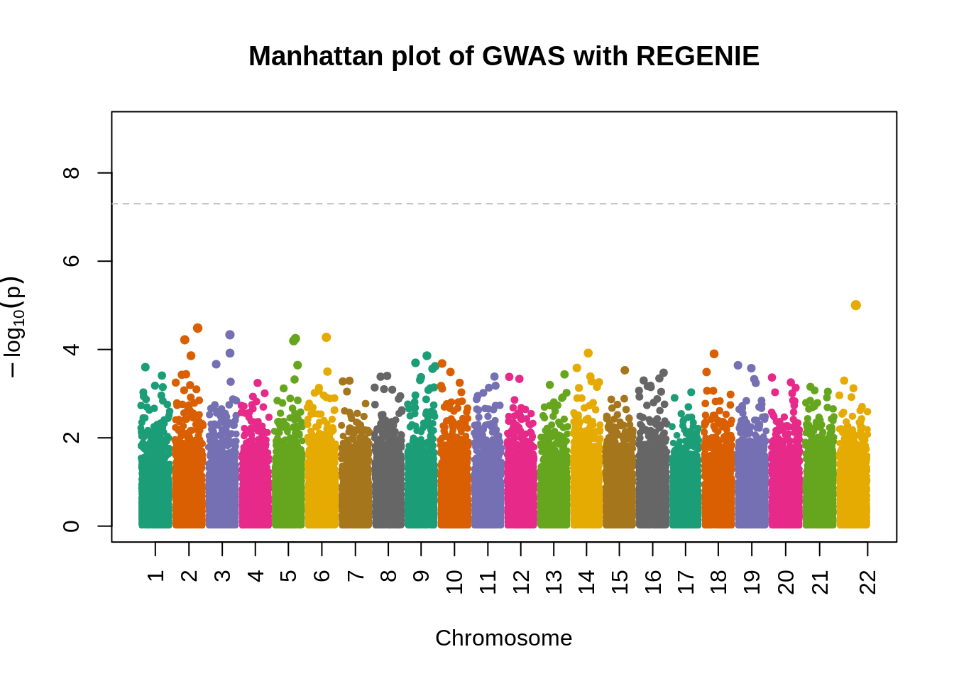
fwrite("plink_gwas.snplist", col.names = FALSE, quote = FALSE)system("/data/SISG2023M15/exe/regenie --bed /data/SISG2023M15/data/sim_rels_geno --phenoFile /data/SISG2023M15/data/sim_rels_pheno.txt --step 2 --bsize 400 --qt --pred regenie_step1_pred.list --extract plink_gwas.snplist --out regenie_step2")- Generate Manhatthan and Q-Q plots based on the association results and compute \(\lambda_{GC}\). Compare with output from Questions 4-6.
regenie.gwas <- fread("regenie_step2_Pheno.regenie", header = TRUE)
regenie.gwas %>% str
Classes 'data.table' and 'data.frame': 105886 obs. of 13 variables:
$ CHROM : int 1 1 1 1 1 1 1 1 1 1 ...
$ GENPOS : int 12000011 12000012 12000019 12000027 12000036 12000061 12000073 12000074 12000117 12000136 ...
$ ID : chr "1:12000011:A:C" "1:12000012:A:C" "1:12000019:T:C" "1:12000027:C:T" ...
$ ALLELE0: chr "C" "C" "C" "T" ...
$ ALLELE1: chr "A" "A" "T" "C" ...
$ A1FREQ : num 0.12 0.187 0.402 0.12 0.415 ...
$ N : int 2400 2400 2400 2400 2400 2400 2400 2400 2400 2400 ...
$ TEST : chr "ADD" "ADD" "ADD" "ADD" ...
$ BETA : num 0.00851 -0.01943 -0.0747 -0.023 0.01463 ...
$ SE : num 0.0419 0.0346 0.0272 0.0416 0.0275 ...
$ CHISQ : num 0.0413 0.3153 7.5548 0.3058 0.2823 ...
$ LOG10P : num 0.0762 0.2407 2.2229 0.2364 0.2254 ...
$ EXTRA : logi NA NA NA NA NA NA ...
- attr(*, ".internal.selfref")=<externalptr> manhattanPlot(
p = 10^-regenie.gwas$LOG10P,
chromosome = regenie.gwas$CHROM,
thinThreshold = 1e-4,
main= "Manhattan plot of GWAS with REGENIE"
)
qqPlot(
  pval = 10^-regenie.gwas$LOG10P,
  thinThreshold = 1e-4,
  main= "Q-Q plot of GWAS with REGENIE"
 )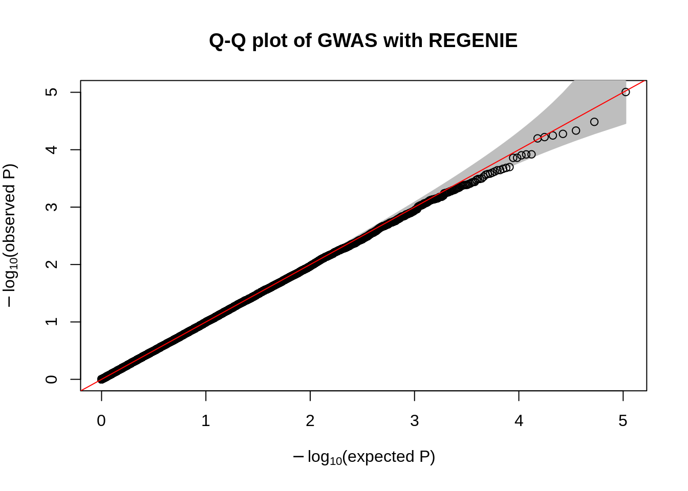
chisq.stats <- qchisq(10^-regenie.gwas$LOG10P, df = 1, lower.tail = FALSE)
median(chisq.stats) / qchisq(0.5,1)
[1] 0.9962878
sessionInfo()R version 4.3.1 (2023-06-16)
Platform: x86_64-pc-linux-gnu (64-bit)
Running under: Ubuntu 22.04.2 LTS
Matrix products: default
BLAS: /usr/lib/x86_64-linux-gnu/blas/libblas.so.3.10.0
LAPACK: /usr/lib/x86_64-linux-gnu/lapack/liblapack.so.3.10.0
locale:
[1] LC_CTYPE=C.UTF-8 LC_NUMERIC=C LC_TIME=C.UTF-8
[4] LC_COLLATE=C.UTF-8 LC_MONETARY=C.UTF-8 LC_MESSAGES=C.UTF-8
[7] LC_PAPER=C.UTF-8 LC_NAME=C LC_ADDRESS=C
[10] LC_TELEPHONE=C LC_MEASUREMENT=C.UTF-8 LC_IDENTIFICATION=C
time zone: Etc/UTC
tzcode source: system (glibc)
attached base packages:
[1] stats graphics grDevices utils datasets methods base
other attached packages:
[1] ggplot2_3.4.2 GWASTools_1.46.0 Biobase_2.60.0
[4] BiocGenerics_0.46.0 tidyr_1.3.0 dplyr_1.1.2
[7] data.table_1.14.8
loaded via a namespace (and not attached):
[1] tidyselect_1.2.0 farver_2.1.1 blob_1.2.4
[4] gdsfmt_1.36.1 fastmap_1.1.1 promises_1.2.0.1
[7] digest_0.6.33 rpart_4.1.19 lifecycle_1.0.3
[10] survival_3.5-5 RSQLite_2.3.1 magrittr_2.0.3
[13] compiler_4.3.1 rlang_1.1.1 sass_0.4.6
[16] tools_4.3.1 utf8_1.2.3 yaml_2.3.7
[19] knitr_1.43 labeling_0.4.2 bit_4.0.5
[22] withr_2.5.0 workflowr_1.7.0 purrr_1.0.1
[25] GWASExactHW_1.01 nnet_7.3-19 grid_4.3.1
[28] fansi_1.0.4 git2r_0.32.0 jomo_2.7-6
[31] colorspace_2.1-0 mice_3.16.0 scales_1.2.1
[34] iterators_1.0.14 MASS_7.3-60 cli_3.6.1
[37] rmarkdown_2.23 generics_0.1.3 rstudioapi_0.15.0
[40] minqa_1.2.5 DBI_1.1.3 DNAcopy_1.74.1
[43] cachem_1.0.8 stringr_1.5.0 operator.tools_1.6.3
[46] splines_4.3.1 vctrs_0.6.3 boot_1.3-28
[49] glmnet_4.1-7 Matrix_1.5-4.1 sandwich_3.0-2
[52] SparseM_1.81 jsonlite_1.8.7 bit64_4.0.5
[55] quantsmooth_1.66.0 mitml_0.4-5 foreach_1.5.2
[58] jquerylib_0.1.4 glue_1.6.2 nloptr_2.0.3
[61] pan_1.8 codetools_0.2-19 gtable_0.3.3
[64] stringi_1.7.12 shape_1.4.6 later_1.3.1
[67] munsell_0.5.0 lmtest_0.9-40 lme4_1.1-34
[70] tibble_3.2.1 pillar_1.9.0 htmltools_0.5.5
[73] quantreg_5.95 R6_2.5.1 formula.tools_1.7.1
[76] rprojroot_2.0.3 evaluate_0.21 lattice_0.21-8
[79] highr_0.10 backports_1.4.1 memoise_2.0.1
[82] broom_1.0.5 httpuv_1.6.11 bslib_0.5.0
[85] MatrixModels_0.5-1 Rcpp_1.0.11 nlme_3.1-162
[88] mgcv_1.8-42 logistf_1.25.0 whisker_0.4.1
[91] xfun_0.39 fs_1.6.2 zoo_1.8-12
[94] pkgconfig_2.0.3